Analyzing, Modeling, and Utilizing Observation Series Correlation in Capital Markets

Abstract

In this paper, we consider the task of the analysis, modeling, and application of dependencies between asset quotes at various capital markets. As an example, we study the dependency between financial instrument observation series in the currency and stock markets. Our work intends to give a theoretical basis to asset management strategies that estimate an asset’s price via regression, taking into account its correlated assets in various markets. Furthermore, we provide a way to increase the estimate quality using an evolutionary algorithm.

1. Introduction

The majority of prominent news in economics, politics, and other areas influences asset quotations and integral trading indicators in various capital markets. This fact makes it possible to hypothesize a significant correlation between these numerical indicators of market trade. In turn, the presence of correlation creates a background for developing asset management strategies based on it.

An obvious version of such a strategy is the ability to promptly estimate the price of the used instrument used with multivariate statistical analysis. If an asset is either under- or over-priced in relation to its market value, a probabilistic conclusion on its quotation dynamics can be drawn. This, in turn, gives rise to constructing various proactive management strategies based on regressor selection, i.e., market parameters used for the multiregression estimation of a financial instrument’s value, the width of the sliding window used for constructing statistical estimates, and other factors.

The theoretical basis of this management strategy is the hypothesis that various capital market asset quotations significantly correlate, as well as the assumption that correlation change dynamics are less variable than the changes in asset quotations.

The considered approach to the analysis and application of financial instrument quotation dependencies is focused on the stochastic chaos model, in which the conditions of stationarity and ergodicity of observation series do not hold [1,2,3,4]. In this case, conventional statistical forecast quality estimates are inherently nonoptimal, and the only available research method is a numerical comparative analysis run on a sufficiently large testing polygon. The current article is dedicated to the investigation of this issue.

Further research directions in the area of dependencies between financial instruments include the analysis of inter-market connections, presented in works such as [5,6,7,8]. This approach opens a wide perspective for constructing forecast algorithms that take into account the higher inertia of integral financial dynamics indicators. The subjects of this research are the evaluation of the efficiency of multivariate statistical analysis in conditions of chaotic dynamics, as well as the application of specialized econometric approaches used for analyzing causal relationships (for example, Granger causality [9]).

2. Methods

Let $X=\left(x_i,i=1,\dots ,m\right)$ be a quotation state vector formed by m parameters. Its individual components may pertain to different capital markets. In this case, the observation matrix $X_k=\left[x_{ik}, i=1,\dots ,m; k=1,\dots n\right]$ will define a vector-valued random process with a discrete time that reflects the dynamics of market asset quotations.

The most widely adopted direct vector observation model [10,11,12,13] is an additive scheme of the following form

$$Y_k=X_k+v_k, k=1,\dots ,n$$

where $X_k, k=1, \dots ,n$ is a systemic component (i.e., used for the analysis and development of management strategies), and $v_k, k=1,\dots n$ is noise.

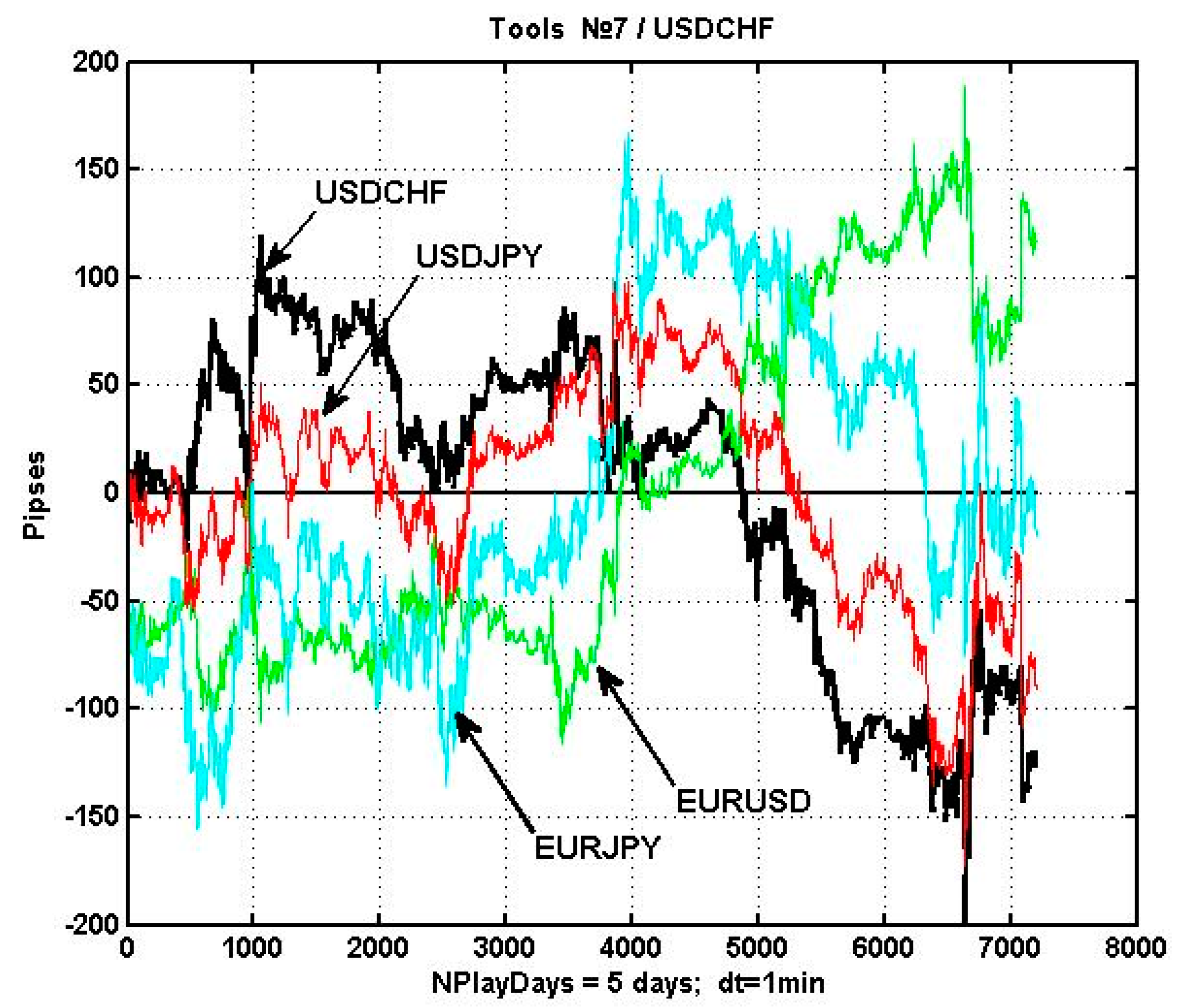
An example of process $Y_k, k=1,\dots n$ shown by the USDCHF, EURUSD, EURJPY, and USDJPY quotations on a five-day observation interval with equidistanced counts dt = 1min can be seen in Figure 1.

It can be easily seen that the systemic component $X_k, k=1, \dots ,n$ is an oscillatory nonperiodic process with a large number of local trends. In the general theory of dynamic processes, such observations are classified as chaotic [1,2,3,4]. The noise $v_k, k=1,\dots n$ is a nonstationary process roughly described by the Gaussian model with changing parameters. A more detailed justification of this model can be found in [1,3,14].

The presence of a chaotic structure in observation series of market assets contradicts the simplest quotation model based on a stationary Gaussian process. Violating the probabilistic analysis’ principal statement on the reproducibility of experience significantly obstructs the usage of otherwise well-applied methods. This is due to an inherent violation of conditions in which the existing computational schemes produce optimal results. This makes conventional analytic methods of evaluating algorithm efficiency almost not applicable. In this case, numerical studies of large observation samples become the main tool for analyzing the efficiency of estimation and management.

At the same time, useful patterns can also be found in trading asset quotation dynamics, as they are represented by multivariate observation series. As it will be shown below, increasing the observation interval used for estimating the correlation reveals strong dependencies between financial instruments. This gives rise to an ability to obtain a regression estimate of the managed asset’s value using its correlated observations. In this case, it is possible to construct an indicator of the discrepancy between the market value and the estimated value of the asset, which may indicate a potential change in the quotation’s direction. In other words, this allows for forecasting the price dynamics using regression.

Let us now move on to correlational analysis of changes in the state of stock and currency markets. We used the most widespread currency pairs, as well as two stock market indicators, as the parameters for the observation vector. Their list can be seen in

Table 1. Financial instruments and their respective numbers.

Financial Instruments
1	2	3	4	5	6
EURUSD	EURJPY	EURGBP	EURCHF	EURCAD	USDCAD
7	8	9	10	11	12
USDCHF	USDJPY	GBPCHF	GBPJPY	GBPUSD	GBPUSD
13	14	15	16	17	18
AUDUSD	CHFJPY	NZDUSD	NZDJPY	FTSE	DJ

. Further on, they will be denoted by their numbers in the table in the text.

We represent the stock market asset observation series as a rectangular table X of size <n:m>, in which n is the number of observations (rows) and m is the number of the observed financial instruments (columns). In this case, the covariation matrix is given by a known equation $\mathrm{cov}(X)=X^{T}X/\left(n-1\right)=\left[p_{ij}, i,j=1,\dots ,m\right]$. The corresponding correlation matrix estimate is given by pairwise correlations $R=\left\{r_{ij}, i,j=1,\dots ,m\right\}$, where $r_{ij}=p_{ij}/\sqrt{p_{ii}{p}_{jj}}$.

The estimates of the pairwise correlations between the stock indexes and the selected currency instruments for three 30-day intervals and one common 90-day interval are presented in

Table 2. Estimates of pairwise correlations between selected stock indexes and currency instruments.

Intervals (Days)	Currency Instruments and FTSE Correlations
Days 1–30	0.147	0.951	0.334	0.908	0.113	0.049	0.256	0.703
	0.019	0.491	−0.388	0.686	0.332	0.892	−0.311	0.519
Days 31–60	−0.697	−0.075	−0.376	0.868	−0.894	−0.502	0.829	0.688
	0.700	0.235	−0.627	0.785	0.502	−0.738	−0.621	−0.054
Days 61–90	−0.431	−0.803	−0.113	0.437	−0.729	0.501	0.524	0.478
	0.335	0.772	−0.458	−0.720	0.109	0.868	0.689	0.645
Days 1–90	−0.066	0.074	0.307	0.586	−0.223	−0.258	0.480	0.103
	0.286	−0.094	−0.480	0.155	0.214	−0.348	0.009	0.238
	Currency Instruments and DJ Correlations
Days 1–30	0.428	0.520	0.655	0.508	0.6181	0.637	−0.160	0.129
	−0.452	−0.169	−0.605	−0.045	−0.271	0.468	−0.316	−0.060
Days 31–60	−0.672	0.172	−0.614	0.821	−0.477	0.047	0.795	0.859
	0.819	0.597	−0.314	0.603	0.085	−0.518	−0.371	0.331
Days 61–90	−0.625	−0.743	−0.252	0.401	−0.746	−0.411	0.676	−0.308
	0.396	−0.680	−0.593	−0.632	−0.277	−0.807	0.558	0.616
Days 1–90	−0.081	−0.255	0.187	0.278	−0.147	−0.139	0.262	−0.215
	0.100	−0.403	−0.343	−0.220	−0.174	−0.590	0.290	0.092

.

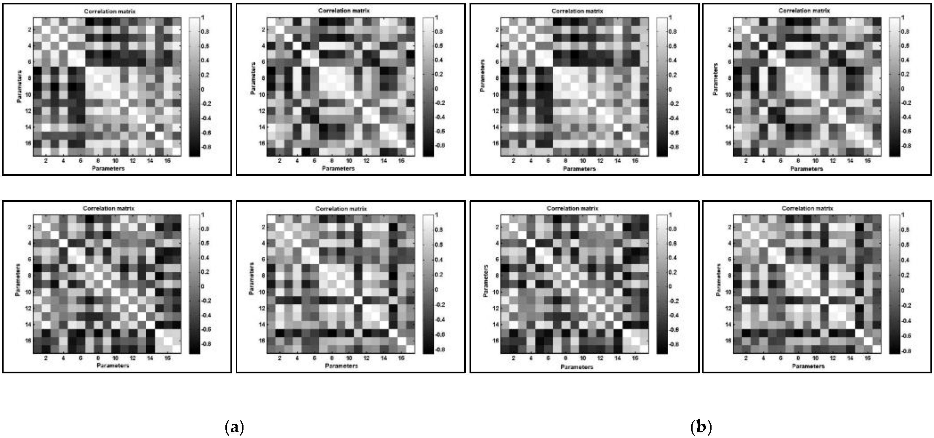
The correlations between the currency pairs from Table 1 and the FTSE and DJ indexes are presented as tonal matrices in Figure 2a,b. The estimates were performed using the time intervals drawn from Table 2.

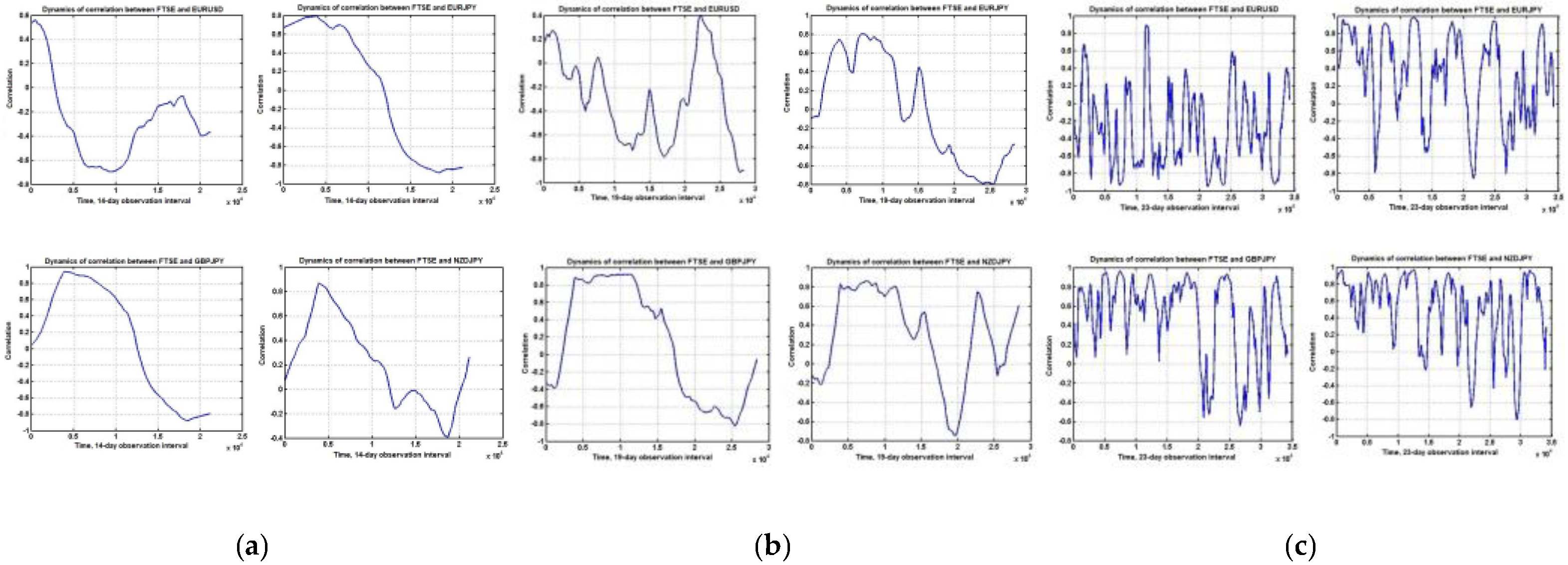
In order to select regressors, it is important to know not only the values of the pairwise correlations, but also their dynamic properties. We estimated the pairwise correlations looping over time within a sliding observation window. The respective computation examples are presented in Figure 3. The presented plots show that the estimated correlation values become highly variable as the observation interval changes.

We selected EURUSD, EURJPY, GBPJPY, and NZDJPY as our currency instruments, setting the lengths of the sliding windows to 10, 5, and 1 observation days. Pairwise correlations between the currency instruments and the FTSE index of the London Stock Exchange were considered as an example.

The presented calculations show that decreasing the size of the observation window leads to a significant increase in variability of the pairwise correlations. Consequently, employing multiregressional analysis for “fast” asset management, such as intraday trading, would not be efficient.

Using a sliding window larger than five days reveals intervals with relatively stable correlation estimates. In such cases, these financial instruments can be used as regressors for estimating the managed indicators.

An immutable set of predictors cannot guarantee an efficient regression estimate for the indicators. This makes it necessary to structurally adapt the regression function to the correlational market changes.

Further enlargement of the sliding window increases the stability of pairwise correlations, but disables the ability to react flexibly to possible variations in the correlations. A smaller sliding window increases the forecast quality, but may lead to false alarm errors caused by the fluctuating properties of the initial processes. Using robust processing algorithms is one of the ways of resolving this contradiction [15,16,17].

The rest of the section will be dedicated to the formal problem setting for asset management using multivariate correlation. Let $Y_k=\left(y_k, k=1,\dots n\right)$ be a quotation vector of the financial instrument, $X_k=\left[x_{ki}, i=1,\dots ,m; k=1,\dots n\right]$, a matrix that contains quotations correlated with $Y_k$ and used as a regressor for forecasting the financial instrument.

The conventional multivariate regression model of a sequential financial instrument price forecast has the form [18,19]

$${\widehat{Y}}_k={\displaystyle \sum }_{j=1}^m{c}_{kj}{x}_{kj}+v_k, k=1,\dots ,n.$$

The most common way of constructing such a forecast is multivariate linear regression (multiregression) based on the least squares method (LSM) [20,21,22]. Because of the data’s chaotic nature and fast loss of relevancy, the estimate of the transfer coefficient of the LSM filter is constructed using a sliding window $Y_{k-L,k}=\left(y_{k-L},\hspace{0.17em}{y}_{k-L+1,}\hspace{0.17em}\dots ,\hspace{0.17em}{y}_k\right) k=1,\dots n$.

Using the following matrix notation

$$C_k={(c_1,c_2,\dots ,c_m)}_k^T, v_k={\left(v_1,v_2,\dots ,v_m\right)}_k^T,$$

$$X_{\left(k-L,k\right)}=\left(\begin{array}{cccc}1& x_{k-L,1}& \cdots & x_{k-L,m}\\ 1& x_{k-L+1,1}& \cdots & x_{k-L+1,m}\\ ⋮& ⋮& \cdots & ⋮\\ 1& x_{k,1}& \cdots & x_{k,m}\end{array}\right)$$

and the conventional minimization of the square error $v_k^T{v}_k={(Y_{k-L,k}-X_{k-L,k}^{T}C)}^T\left(Y_{k-L,k}-X_{k-L,k}^{T}C\right)=min$, we obtain the well-known relation used for estimating the transfer coefficient of the LSM filter of form ${\hat{C}}_k={(X_{k-L,k}^T{X}_{k-L,k})}^{-1}{X}_{k-L,k\_}^T{Y}_{k-L,k}$.

Thus, at each step of observing the state of the market, we have the value of the current asset price $y_k$ and its estimate ${\widehat{y}}_k={\hat{C}}_k{X}_{k-L,k}$, constructed using the values of the observed correlated financial instruments. The value of $d_k={\widehat{Y}}_k-Y_k$ is an oscillatory indicator of the under- or over-price of the current asset that allows for forecasting the direction of its quotation.

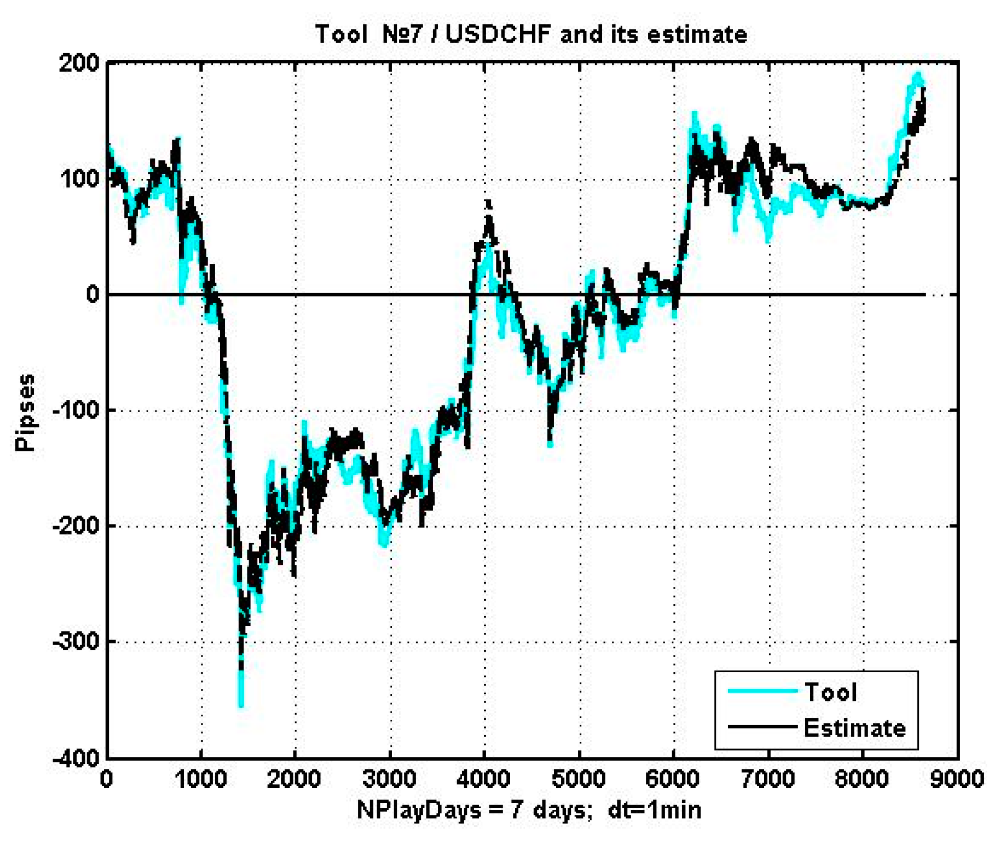
As an illustration, Figure 4 contains the observation plots of USDCHF in a seven-day period with an observation interval of 1 min, as well as its regression forecast constructed with the use of correlated quotations of EURUSD, EURJPY, and USDJPY.

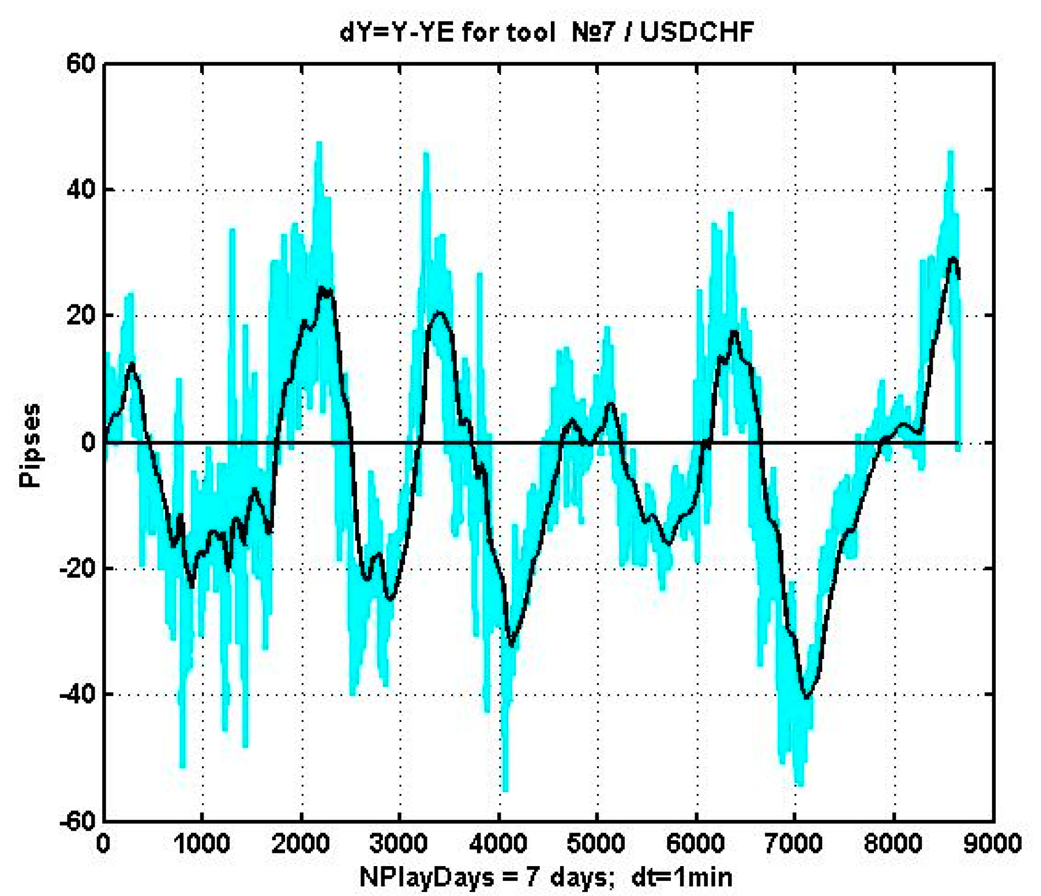
Figure 5 presents the difference $d_i, i=1,\dots ,n$ between the quotations of USDCHF and their regression estimates, as well as the smoothed version, obtained via applying an exponential filter with a transfer coefficient of $\alpha =0.05$.

Let us now consider the simplest application of this difference to the construction of an asset management strategy.

3. Results

3.1. Multiregressional Data Analysis-Based Management Strategy Constructed upon Financial Instrument Correlation

The simplest asset management strategy based on computational regression estimates can be constructed with the following criterion $K: \left|d_k\right|>d\ast ,k=1,\dots ,n.$

If $d_k>d\ast$, this means $Y_i>{\widehat{Y}}_i$, i.e., the financial instrument is overpriced, and its price can be expected to go down. Vice versa, if $d_i<-d\ast$, i.e., $Y_i<{\widehat{Y}}_i$, indicates underpricing and therefore the price should go up. A statistical approach produces solutions that are correct only to a certain confidence level. Critical values of $d\ast$ are determined by its distribution tables (or a statistic constructed upon it with a known distribution law). In the conditions of nonstationary dynamics with a chaotic systemic component, such an approach is unfeasible. The critical value has to be selected based on the preliminary analysis of the retrospective information drawn from a large observation interval.

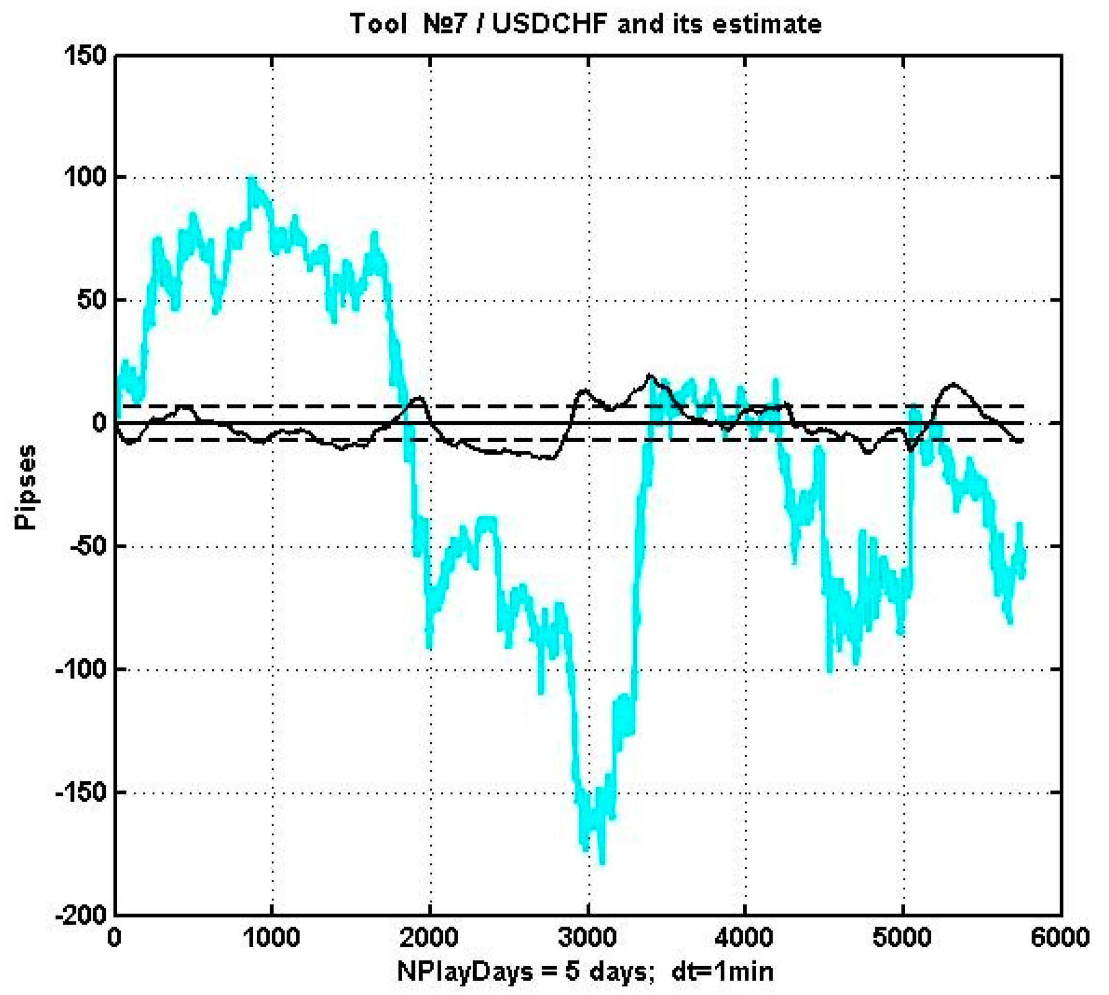
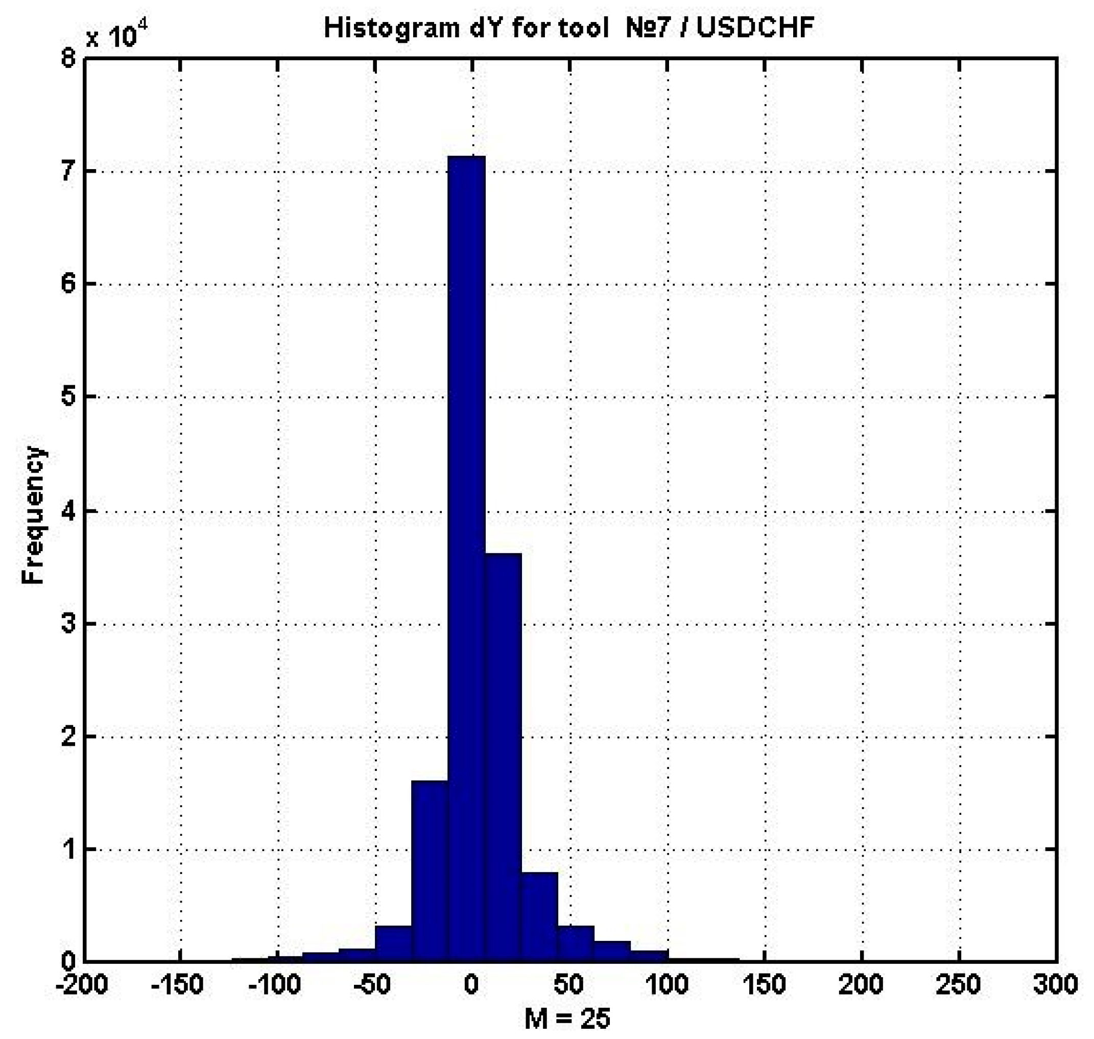
As an example, let us consider how $d_k={\widehat{Y}}_k-Y_k$ changes for USDCHF on a five-day observation interval with 1-min counts. The respective plot, the smoothed version of $d_k={\widehat{Y}}_k-Y_k$, and the decision levels are presented in Figure 6. For better understandability, the value of the oscillator and its critical value are enlarged by 1.5 times. Figure 7 contains a histogram of $d_k, k=1,\dots ,n$, which demonstrates a weak convergence of the given difference’s distribution to the Gaussian law.

.

According to the described management strategy, if the oscillator surpasses the threshold value, i.e., $d_s\left(t\right)>d_s^{\ast }$, one can open a long position. Alternatively, a short position can be opened if $d_s\left(t\right)<-d_s^{\ast }$. Positions can be closed along with a reverse crossing of the threshold $d_s^{\ast }$, or by the conventional method of setting the “take profit” and “stop loss” levels.

Figure 6 shows that there is no stable trend for either underprice or overprice. The reason for this is clear: the oscillator’s movement into either direction is determined by its estimate of the prices of financial instruments used as regressors. At the same time, there are external factors that lead to the appearance of dynamic trends. The sum of these movements produces the final form of the dynamics, the direction of which is determined by a vector sum of heterogeneous and hardly forecasted influencing factors. Because of this, our asset management strategy algorithm has to be adapted further to consider the additional external impact factors of the financial instrument’s price.

3.2. Evolutionary Adaptation of Our Multiregressional Asset Management Strategy Algorithm

A natural development of the presented study lies in solving the issue of whether a winning regression estimate strategy exists. This requires adapting the parameters of the management algorithm in order to obtain the most positive result. It is impossible to obtain a strict solution to an optimization problem in the conditions of chaotic dynamics. Because of this, we implemented a numerical iterative optimization based on evolutionary modeling [23,24,25,26,27,28]. In essence, this method was a modification of random search inspired by Darwinian evolution [23]. An example of how evolutionary modeling can be applied to optimize a management strategy can be found in [24].

A base algorithm of sequential adaptation is characterized by an array of modifiable parameters that form a genome vector $G=\left[g_1,\hspace{0.17em}{g}_2,\dots ,\hspace{0.17em}{g}_{mg}\right]$. In structural adaptation, the genome also contains the numbers of the regressors used for the estimation.

The criterion for opening a position during asset management, as was said previously, is $K: \left|{\tilde{d}}_k\right|>B$, where ${\tilde{d}}_i$ is the smoothed value of the difference between the current estimate and value of the observed process.

The starting value of the genome $G_0 = {[g_1,\hspace{0.17em}{g}_2,\dots ,\hspace{0.17em}{g}_{mg}]}_0$ is estimated based on the results of the preliminary numerical analysis of the retrospective data. As threshold values, we used standard deviations (SDs) of the modified parameter observations on the specified interval.

The functional block diagram of the evolutionary adaptation of the asset value estimation algorithm is presented in Figure 8. Within the current study, we employed the following three parametric genome modifications:

• Little single modification, LSM. This term refers to a small change (within a single SD) in a single randomly selected parameter of the parent genome.
• Little group modification, LGM.
• Strong single mutation, SSM, also known as parametric mutation. This refers to a significant modification (within three SDs) of a single randomly selected parameter.

The first generation of parent genomes was formed via applying LSM modifications to $G_0$. Next, using every mentioned type of modification, we created a group of child genomes, which, combined with their parents, constitute the first generation of our estimation algorithm parameters. The next step is, in accordance to the computational scheme shown in Figure 8, testing every modified version of the algorithm on a polygon of retrospective data. The result of the testing is evaluated using the terminal indicator of the quality of management, i.e., the gain. Next, all of the genome versions are ordered by their profit. During the selection process, the genomes with the least efficiency values are pruned, and the best genomes become the parents of the next generation. Next, looping over the generations, the versions are modified and selected, i.e., they are sequentially adapted to the particularities of the currently observed asset quotation fragments. Theoretically rigorous optimality of the found solutions is not guaranteed. However, the gain value cannot decrease as the number of generations increases. Furthermore, the presence of parametric and structural mutations allows for carrying the adaptation process out of local extrema vicinities.

Note that in contrast with random search, every iteration preserves a finite group of genomes instead of a single best solution. This approach allows for obtaining the best terminal solution using sequences of intermediate nonoptimal solutions.

3.3. An Evolutionally Adapted Implementation of a Regression Asset Management Strategy

Let us present a numerical example of using evolutionary adaptation for the regression asset management task. Consider USDCHF as the managed asset, and EURUSD, EURJPY, and USDJPY as regressors.

We used the parameter vector $G=\left[nW,\hspace{0.17em}\alpha ,\hspace{0.17em}B\right]$ as the genome, where $nW$ is the size of the sliding window of data used to construct regression estimate ${\widehat{Y}}_k$, $\alpha$ is the transfer coefficient of the smoothing exponential filter, and $B$ is the boundary (critical) value used in the solution-making during asset management. The starting values of the modified parameters $G_0=\left[0.5,\hspace{0.17em}0.03,\hspace{0.17em}4\right]$ are estimates based on USDCHF quotation dynamics analysis for 1-year interval and minute counts. The first parameter is evaluated in days, the second one is dimensionless, and the third one is measured in pipses. The intervals of allowed variation in the genome parameters are defined by matrix

$$\mathsf{\Delta }G = \left[\begin{array}{cc}0.1& 10\\ 0.001& 1\\ 1& 30\end{array}\right]$$

We used from 7 to 10 generation changes for evolutionary adaptation, preserving the $N_a=4$ parent genomes each time. For each parent, we performed three LSMs, a single LGM for all parameters, and one SSM. Thus, every generation included 24 genome modifications.

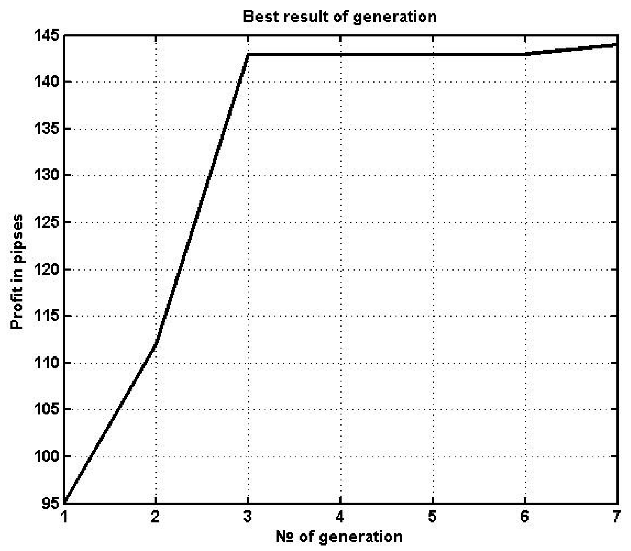
Next, we tested each genome version on the same data polygon. During selection, we preserved the four most successful genomes, making them parents of the next generation. The procedure was run for 7–8 iterations. The plot of the profit for the best solutions can be seen in Figure 9.

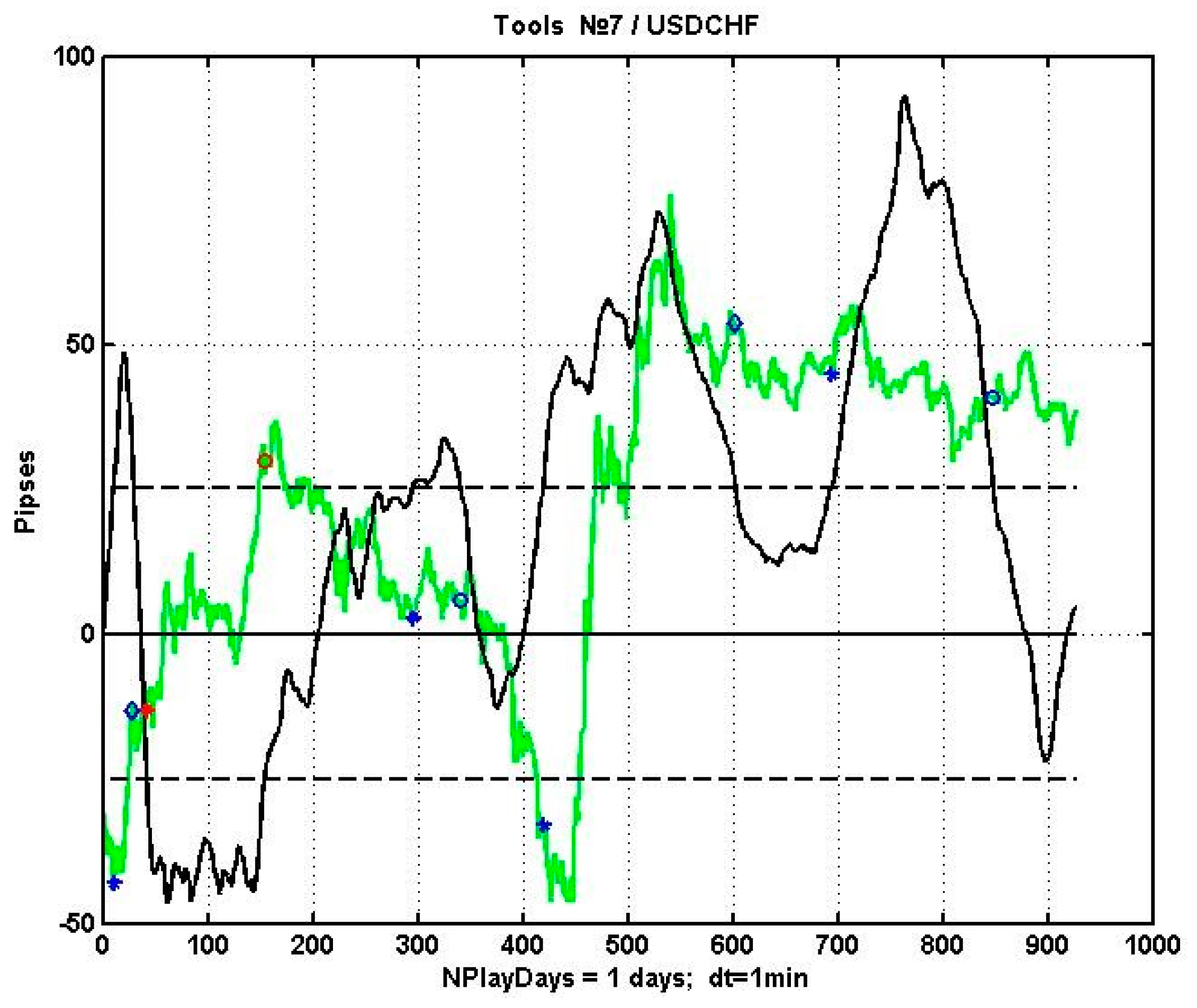
The plot of the implemented regression asset management model that corresponds to the best genome is presented in Figure 10. For a better illustration, we used a short trading interval of 24 h. The plot shows the observed process of quotation dynamics $Y\left(t\right)$, the plot of criterial statistics ${\tilde{d}}_i\left(t\right)$ (enlarged for better understandability), and the decision levels $B$ (horizontal lines).

Stars on line $Y\left(t\right)$ and denote the moments of ${\tilde{d}}_i\left(t\right)$ crossing the $\pm B$ levels, i.e., position opening. Positions were closed at the moments corresponding to the reverse crossing of levels $\pm B$ by ${\tilde{d}}_i\left(t\right)$. The graph denotes these moments either with diamonds (profit gain) or circles (profit loss). It can be seen that the result is not clear-cut: it is rather probabilistic. The provided example has benefitted from our evolutionally adapted regression algorithm by obtaining 140 pipses of profit in a single day.

4. Discussion

The obtained results let us conclude that the chaotic multivariate environment of trading assets contains explicit correlations, the presence of which allows for implementing multiregressional computational schemes for asset management.

Using multiregressional estimates allows for constructing oscillating indicators with an asset management strategy for multivariate chaotic environments, which is an inherent possibility of a positive result.

A significant difference in this approach is the lack of requirement for trend identification and usage. This makes it possible to move away from the conventional method of extrapolation forecasting, which is essential when working with chaotic processes. Further improvement in management quality is provided by evolutionary adaptation.

Using regression analysis allows for directly substituting forecasting a chaotic process with an indirect estimate of the forthcoming price dynamics of the financial instrument price. Such an approach makes the forecast more stable in view of nonstationary variations of quotation dynamics.

It is important to note that the proposed approach, just as with any other oscillator, may lead to a negative result. In particular, an oscillator-based judgement of an instrument’s overprice during a long-lasting positive trend may lead to a loss. These situations can be overcome with a complex solution based on multi-expert management. These issues will constitute the subject of further research.