
An Application of Optimal Control to Sugarcane Harvesting in Thailand

 , , and
Abstract
1. Introduction
2. Mathematical Models
- is the profit for sugarcane cut at time t (baht/day),
- is the total amount of sugarcane (tonnes) on the farms in a region at time t,
- is the maximum rate of cutting sugarcane (tonnes/day),
- is the initial time at start of harvesting season (day),
- is the final time at end of harvesting season (day),
- a is the total amount of sugarcane on farms at the initial time (tonnes),
- is a logistic growth function for the rate of increase in weight of sugarcane (tonnes per day) on the farms in a region at time t, where r is a specific growth rate (1/day), and K is a constant which represents the carrying capacity of the farms in the region (tonnes).
3. Optimization and Optimal Control Methods
3.1. Bi-Objective Optimization
3.2. Quasi-Newton Optimization
3.3. Linear Programming
3.4. Pontryagin Maximum Principle for Continuous Optimal Control
Continuous Optimal Control Algorithm
- Select an initial feasible cutting pattern such that and .
- Solve the state and costate equations for this pattern to obtain values of and . For reasons of numerical stability, the state equations must be integrated forwards in time and the costate equations must be integrated backwards in time.
- Compute the Hamiltonian values and the partial derivative values .
- In our examples, we have found that all partial derivatives are positive. Therefore, if there were no constraints on the state variables, the optimal cutting pattern would be to cut the maximum amount available for cutting each day. In order to satisfy the state variable constraints and , we chose the optimal values as follows.
- (a)
- Sort the derivatives in decreasing order.
- (b)
- Find the number of days M required to cut all available cane at the maximum rate and select the times corresponding to the top M values of the derivatives.
- (c)
- If , set the new cutting pattern with at these M values of and at all other times. However, if , set for the top derivative values andwhere is time of derivative M.Note: A slight modification is required if growth can occur ().
- Then, stop if the new cutting pattern is within a selected tolerance of the old cutting pattern or return to step 2 and repeat if the new pattern is not within the selected tolerance of the old.
3.5. Pontryagin Maximum Principle for Discrete Optimal Control
4. The Commercial Cane Sugar System (CCS) in Thailand
4.1. Price of Sugarcane
- Price based on weight: The basic price per weight of sugarcane (baht/tonne) is fixed by the Royal Thai government for each crop year. This basic price is the same for all regions. However, the actual price paid to farmers for fired sugarcane is 30 baht/tonne less than the basic price. Then, at the end of harvesting for the year, factories in each region will share the total amount of money deducted from fired sugarcane sales in that region to farmers who sold fresh sugarcane at a rate not exceeding 70 baht/tonne of fresh sugarcane delivered. We will use the notation to denote actual price based on weight (baht/tonne) for type i in region j.The actual prices per tonne based on weight for sugarcane for a given crop year are:where is the basic price, is the total amount of fresh sugarcane (tonnes) harvested in region j and is the total amount of fired sugarcane (tonnes) harvested in region j for a given year.
- Price based on sweetness (CCS): Each year, the Royal Thai government sets a basic price per tonne for sugarcane with 10 CCS, where CCS is the percentage by weight of sugar in sugarcane. This price is the same for fresh and fired sugarcane and for all regions. The actual price per tonne received by farmers is then adjusted if the CCS is different from 10. For sugarcane harvested in period k in region j the actual price per tonne for a given year iswhere is the basic price per tonne for sugarcane with 10 CCS set by the government for the year, and , where is the average CCS from sugarcane harvested in period k in region j and the factor 0.06 is the rate of change of price per 1 CCS from the base level of 10.
4.2. Costs of Production
4.3. Total Revenue and Total Profit
4.4. Cutting Constraints
5. Results
5.1. Profits
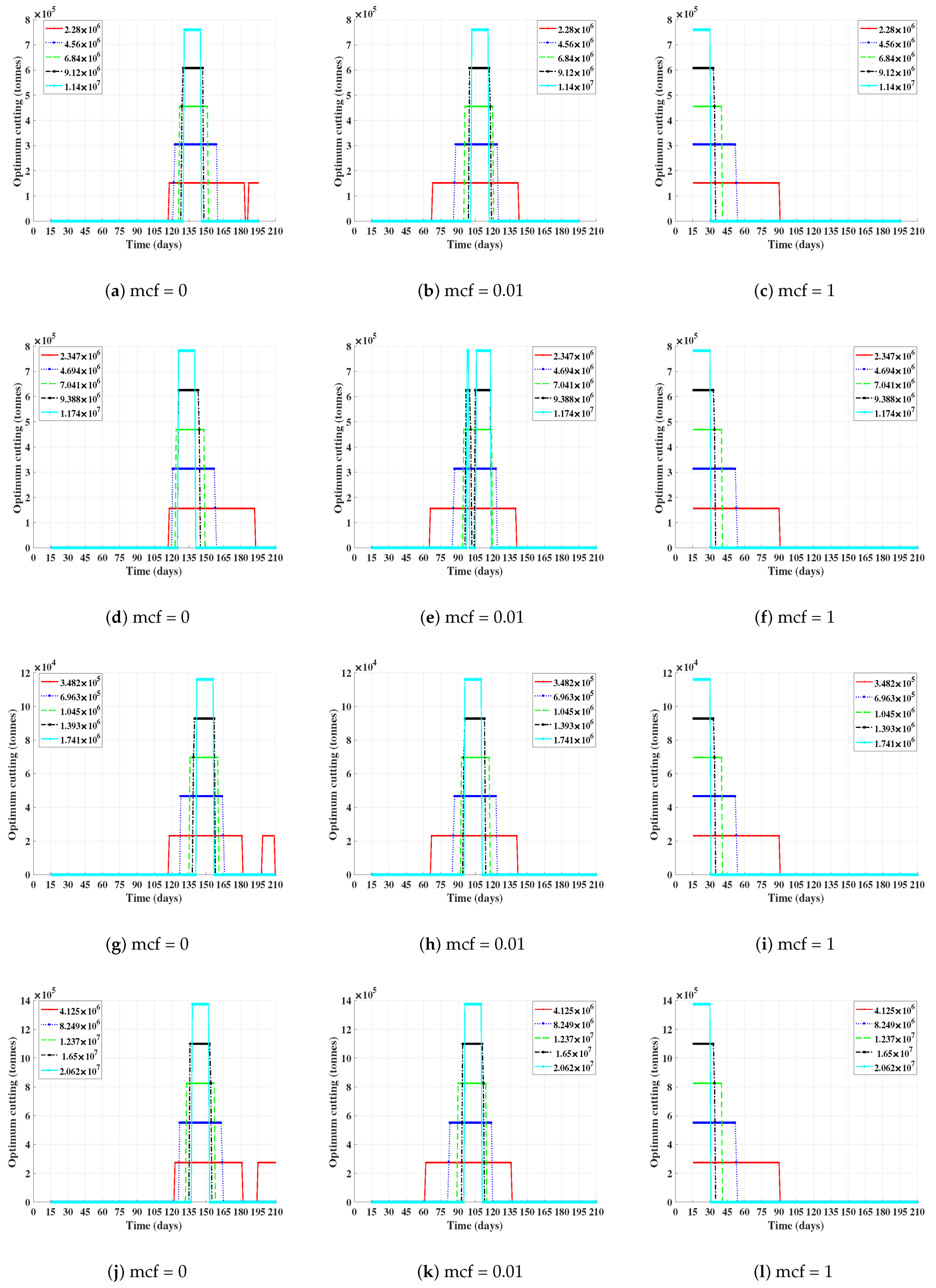
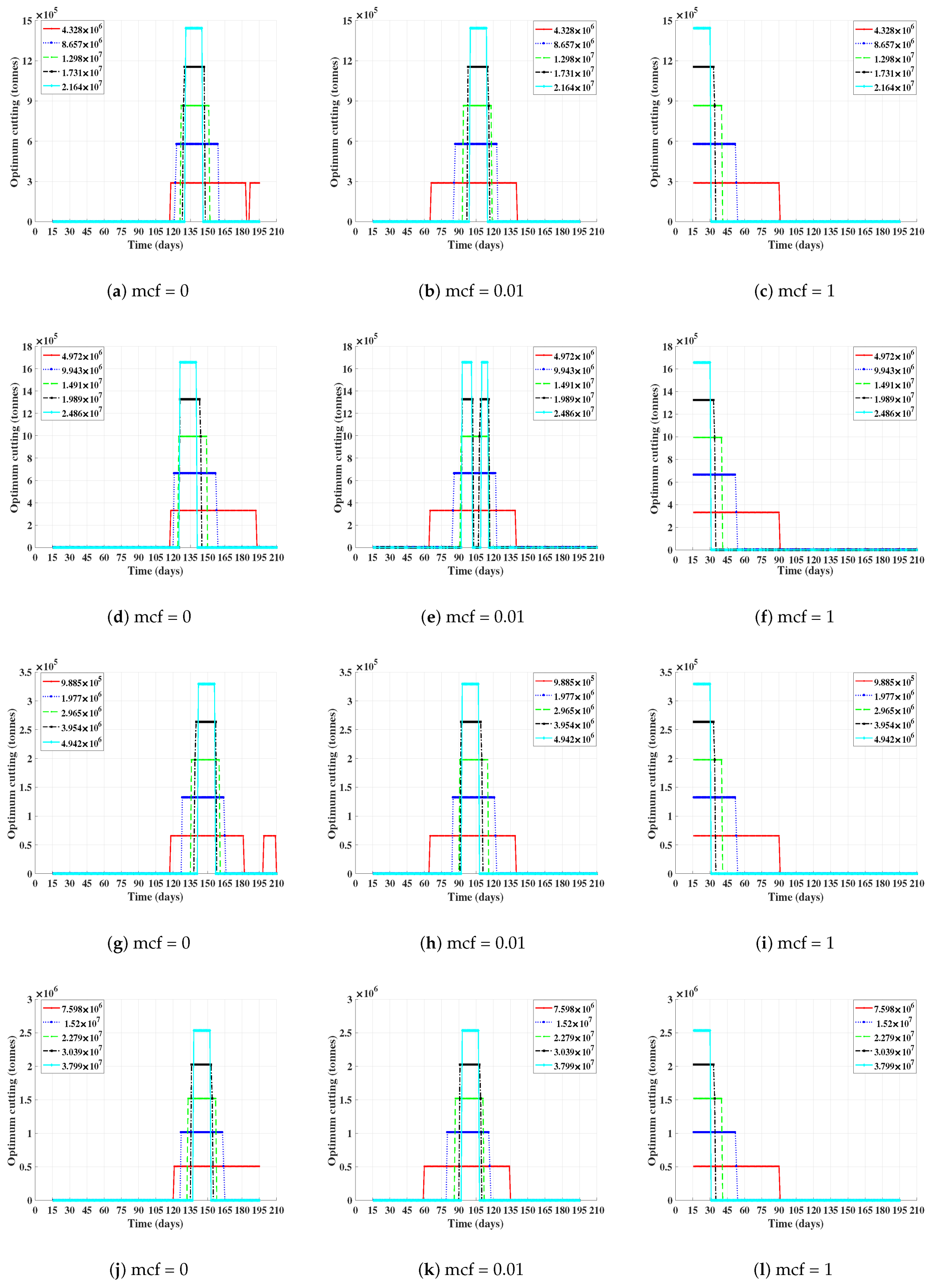
5.2. Optimal Daily Cutting Patterns
5.3. Linear Progamming Dual Variables and Hamiltonian Derivatives
5.4. Computation Times
6. Discussion and Conclusions
Author Contributions
Funding
Institutional Review Board Statement
Informed Consent Statement
Data Availability Statement
Acknowledgments
Conflicts of Interest
References
- Pontryagin, L.S. Mathematical Theory of Optimal Processes; Routledge: Abingdon-on-Thames, UK, 2018. [Google Scholar]
- Luenberger, D.G. Introduction to Dynamic Systems: Theory, Models & Applications; John Wiley & Sons: New York, NY, USA, 1979. [Google Scholar]
- Lenhart, S.; Workman, J.T. Optimal Control Applied to Biological Models; Chapman & Hall/CRC: Boca Raton, FL, USA, 2007. [Google Scholar]
- Deb, K. Multi-Objective Optimization Using Evolutionary Algorithms; John Wiley & Sons: New York, NY, USA, 2005. [Google Scholar]
- Gill, P.E.; Murray, W.; Wright, M.H. Practical Optimization; Wiley-Interscience: Chichester, UK, 1981. [Google Scholar]
- Rao, S.S. Engineering Optimization: Theory and Practice, 4th ed.; Wiley-Interscience: New York, NY, USA, 2009. [Google Scholar]
- Fletcher, R. Practical Methods of Optimization, 2nd ed.; John Wiley & Sons: New York, NY, USA, 2013. [Google Scholar]
- Chvátal, V. Linear Programming; W.H. Freeman: San Francisco, CA, USA, 1983. [Google Scholar]
- The Cane and Sugar Board, Ministry of Industry of Thailand. Data of Sugarcane. 2013. Available online: http://www.ocsb.go.th (accessed on 18 March 2021).
- The Cane and Sugar Board, Ministry of Industry of Thailand. Data of Sugarcane. 2014. Available online: http://www.ocsb.go.th (accessed on 18 March 2021).
- The Cane and Sugar Board, Ministry of Industry of Thailand. Data of Sugarcane. 2015. Available online: http://www.ocsb.go.th (accessed on 18 March 2021).
- The Cane and Sugar Board, Ministry of Industry of Thailand. Data of Sugarcane. 2018. Available online: http://www.ocsb.go.th (accessed on 18 March 2021).
- The Cane and Sugar Board, Ministry of Industry of Thailand. Data of Sugarcane. 2019. Available online: http://www.ocsb.go.th (accessed on 18 March 2021).
- Pornprakun, W.; Sungnul, S.; Kiataramkul, C.; Moore, E.J. Determining optimal policies for sugarcane harvesting in Thailand using bi-objective and quasi-Newton optimization methods. Adv. Differ. Equations 2019, 2019, 1–15. [Google Scholar] [CrossRef]
- Kiataramkul, C.; Wake, G.; Ben-Tal, A.; Lenbury, Y. Optimal nutritional intake for fetal growth. Math. Biosci. Eng. 2011, 8, 723–732. [Google Scholar] [PubMed]
- Dine, W.; Lenhart, S.; Behncke, H. Discrete time optimal harvesting of fish populations with age structure. Lett. Biomath. 2014, 1, 193–207. [Google Scholar] [CrossRef]
- Kiataramkul, C.; Matkhao, P. Optimal Control Problem of Food Intake of Swine During Post Weaning Period. Kasetsart J. (Nat. Sci.) 2015, 49, 983–989. [Google Scholar]
- Puengpao, S.; Kiataramkul, C.; Moore, E.J. Application of discrete optimal control to feeding of farm animals. In Proceedings of the International Conference in Mathematics and Applications (ICMA-MU2016), Bangkok, Thailand, 17–19 December 2016; pp. 151–160. [Google Scholar]
- Gomes, F.R.A. Bi-objective mathematical model for choosing sugarcane varieties with harvest residual biomass in energy cogeneration. Int. J. Agric. Biol. Eng. 2012, 5, 50–58. [Google Scholar]
- Sungnul, S.; Pornprakun, W.; Prasattong, S.; Baitiang, C. Optimal Time of Sugarcane Harvesting for Sugar Factories in Thailand. In Proceedings of the International Conference in Mathematics and Applications (ICMA-MU2016), Bangkok, Thailand, 17–19 December 2016; pp. 185–194. [Google Scholar]
- Sungnul, S.; Pornprakun, W.; Prasattong, S.; Baitiang, C. Multi-Objective Mathematical Model for the Optimal Time to Harvest Sugarcane. Appl. Math. 2017, 8, 329. [Google Scholar] [CrossRef][Green Version]
- Naranong, V.; Tansakun, S.; Chantaprom, T. A Study of Reform of the Structure of Thailand’s Sugar and Cane Industry. Thail. Dev. Res. Inst. 2013. Available online: https://dric.nrct.go.th/index.php?/Search/SearchDetail/278291 (accessed on 18 March 2021).


| Type | Year | Basic Price (baht) | Total Amount (tonnes) | ||||
|---|---|---|---|---|---|---|---|
| North | Central | East | North-East | ||||
| Fresh | 2012/13 | 198.47 | 999.20 | 7.036 | 9.309 | 0.955 | 16.909 |
| 2013/14 | 194.67 | 958.31 | 7.076 | 9.600 | 1.235 | 20.013 | |
| 2014/15 | 197.41 | 900.00 | 7.384 | 9.235 | 1.264 | 19.028 | |
| 2017/18 | 141.00 | 880.00 | 11.399 | 11.735 | 1.741 | 20.623 | |
| 2018/19 | 141.00 | 700.00 | 13.944 | 11.069 | 1.705 | 24.221 | |
| Fired | 2012/13 | 140.00 | 999.20 | 17.562 | 21.189 | 3.731 | 23.311 |
| 2013/14 | 140.00 | 958.31 | 17.134 | 20.479 | 3.237 | 24.892 | |
| 2014/15 | 140.00 | 900.00 | 17.999 | 18.766 | 3.946 | 28.338 | |
| 2017/18 | 140.00 | 880.00 | 21.641 | 24.858 | 4.942 | 37.989 | |
| 2018/19 | 140.00 | 700.00 | 19.163 | 20.468 | 4.174 | 36.226 | |
| Period | North | Central | East | North-East |
|---|---|---|---|---|
| (1) 1–15 December 2017 | 10.387 | 9.932 | 10.482 | 11.655 |
| (2) 16–31 December 2017 | 10.726 | 10.262 | 10.807 | 12.009 |
| (3) 1–15 January 2018 | 11.032 | 10.485 | 10.994 | 12.313 |
| (4) 16–31 January 2018 | 11.378 | 10.856 | 11.367 | 12.596 |
| (5) 1–14 February 2018 | 11.654 | 11.134 | 11.670 | 12.840 |
| (6) 15–28 February 2018 | 11.856 | 11.328 | 11.911 | 13.021 |
| (7) 1–15 March 2018 | 12.005 | 11.463 | 12.075 | 13.174 |
| (8) 16–31 March 2018 | 12.120 | 11.586 | 12.211 | 13.291 |
| (9) 1–15 April 2018 | 12.147 | 11.603 | 12.253 | 13.333 |
| (10) 16–30 April 2018 | 12.139 | 11.595 | 12.265 | 13.337 |
| (11) 1–15 May 2018 | 12.112 | 11.572 | 12.235 | 13.311 |
| (12) 16–31 May 2018 | 12.101 | 11.564 | 12.189 | 13.298 |
| (13) 1–15 June 2018 | 12.101 | 11.561 | 12.187 | 13.298 |
| Period | North | Central | East | North-East |
|---|---|---|---|---|
| (1) 16–30 November 2018 | 9.760 | 9.752 | - | 11.530 |
| (2) 1–15 December 2018 | 10.175 | 10.114 | 11.316 | 11.909 |
| (3) 16–31 December 2018 | 10.486 | 10.322 | 11.641 | 12.163 |
| (4) 1–15 January 2019 | 10.822 | 10.622 | 11.855 | 12.507 |
| (5) 16–31 January 2019 | 11.182 | 10.961 | 12.176 | 12.819 |
| (6) 1–14 February 2019 | 11.444 | 11.213 | 12.404 | 13.036 |
| (7) 15–28 February 2019 | 11.639 | 11.419 | 12.599 | 13.179 |
| (8) 1–15 March 2019 | 11.834 | 11.596 | 12.790 | 13.311 |
| (10) 16–31 March 2019 | 11.986 | 11.654 | 12.858 | 13.427 |
| (11) 1–15 April 2019 | 12.015 | 11.658 | 12.858 | 13.464 |
| (12) 16–30 April 2019 | 12.015 | 11.658 | - | 13.481 |
| (13) 1–15 May 2019 | 12.015 | 11.658 | - | 13.480 |
| Period | North | Central | East | North-East | ||||
|---|---|---|---|---|---|---|---|---|
| Fresh | Fired | Fresh | Fired | Fresh | Fired | Fresh | Fired | |
| (1) 1–15 December 2017 | 1041.45 | 989.76 | 1017.42 | 966.54 | 1046.47 | 994.60 | 1108.38 | 1054.40 |
| (2) 16–31 December 2017 | 1059.32 | 1007.02 | 1034.82 | 983.35 | 1063.59 | 1011.14 | 1127.10 | 1072.48 |
| (3) 1–15 January 2018 | 1075.49 | 1022.63 | 1046.63 | 994.76 | 1073.47 | 1020.68 | 1143.12 | 1087.96 |
| (4) 16–31 January 2018 | 1093.77 | 1040.29 | 1066.19 | 1013.65 | 1093.16 | 1039.70 | 1158.09 | 1102.42 |
| (5) 1–14 February 2018 | 1108.35 | 1054.37 | 1080.86 | 1027.82 | 1109.15 | 1055.15 | 1170.95 | 1114.83 |
| (6) 15–28 February 2018 | 1118.99 | 1064.65 | 1091.12 | 1037.73 | 1121.90 | 1067.46 | 1180.48 | 1124.05 |
| (7) 1–15 March 2018 | 1126.88 | 1072.27 | 1098.26 | 1044.62 | 1130.55 | 1075.82 | 1188.59 | 1131.87 |
| (8) 16–31 March 2018 | 1132.94 | 1078.12 | 1104.74 | 1050.88 | 1137.74 | 1082.76 | 1194.75 | 1137.83 |
| (9) 1–15 April 2018 | 1134.36 | 1079.49 | 1105.62 | 1051.74 | 1139.97 | 1084.91 | 1197.00 | 1140.00 |
| (10) 16–30 April 2018 | 1133.94 | 1079.09 | 1105.23 | 1051.36 | 1140.58 | 1085.50 | 1197.20 | 1140.19 |
| (11) 1–15 May 2018 | 1132.52 | 1077.72 | 1104.02 | 1050.19 | 1139.02 | 1084.00 | 1195.82 | 1138.86 |
| (12) 16–31 May 2018 | 1131.96 | 1077.17 | 1103.56 | 1049.75 | 1136.59 | 1081.65 | 1195.14 | 1138.21 |
| (13) 1–15 June 2018 | - | - | 1103.43 | 1049.62 | 1136.46 | 1081.53 | 1195.14 | - |
| Period | North | Central | East | North-East | ||||
|---|---|---|---|---|---|---|---|---|
| Fresh | Fired | Fresh | Fired | Fresh | Fired | Fresh | Fired | |
| (1) 16–30 November 2018 | 830.94 | 780.37 | 830.57 | 780.02 | - | - | 905.28 | 851.52 |
| (2) 1–15 December 2018 | 848.33 | 797.02 | 845.77 | 794.57 | 896.29 | 842.92 | 921.17 | 866.73 |
| (3) 16–31 December 2018 | 861.41 | 809.54 | 854.53 | 802.95 | 909.92 | 855.97 | 931.83 | 876.94 |
| (4) 1–15 January 2019 | 875.51 | 823.03 | 867.13 | 815.01 | 918.92 | 864.58 | 946.27 | 890.76 |
| (5) 16–31 January 2019 | 890.66 | 837.53 | 881.37 | 828.64 | 932.40 | 877.48 | 959.39 | 903.32 |
| (6) 1–14 February 2019 | 901.66 | 848.06 | 891.93 | 838.75 | 941.96 | 886.63 | 968.51 | 912.05 |
| (7) 15–28 February 2019 | 909.83 | 855.88 | 900.58 | 847.03 | 950.17 | 894.49 | 974.52 | 917.80 |
| (8) 1–15 March 2019 | 918.04 | 863.74 | 908.04 | 854.16 | 958.17 | 902.15 | 980.06 | 923.10 |
| (10) 16–31 March 2019 | 924.40 | 869.82 | 910.46 | 856.48 | 961.05 | 904.91 | 984.95 | 927.78 |
| (11) 1–15 April 2019 | 925.61 | 870.99 | 910.66 | 856.67 | 961.05 | 904.90 | 986.50 | 929.26 |
| (12) 16–30 April 2019 | - | - | 910.66 | 856.67 | - | - | 987.18 | 929.92 |
| (13) 1–15 May 2019 | - | - | - | - | - | - | 987.18 | 929.91 |
| Year | Region | Harvesting Cost (baht/tonne) | Transport Cost (baht/tonne) | Maintenance Cost (baht/tonne) |
|---|---|---|---|---|
| 2012/13 | North | 924.28 | 136.51 | 52.70 |
| Central | 872.95 | 147.66 | 94.24 | |
| East | 836.25 | 148.89 | 92.51 | |
| North-east | 765.18 | 141.97 | 56.30 | |
| 2013/14 | North | 815.89 | 149.46 | 66.07 |
| Central | 781.41 | 147.04 | 86.59 | |
| East | 912.61 | 165.66 | 106.01 | |
| North-east | 875.84 | 151.64 | 59.55 | |
| 2014/15 | North | 1061.42 | 182.36 | 79.38 |
| Central | 954.16 | 155.30 | 82.32 | |
| East | 1024.71 | 194.89 | 94.30 | |
| North-east | 987.00 | 140.12 | 91.71 | |
| 2017/18 | North | 771.27 | 143.62 | 84.94 |
| Central | 771.91 | 137.22 | 84.83 | |
| East | 848.51 | 146.21 | 102.43 | |
| North-east | 871.78 | 150.74 | 66.80 | |
| 2018/19 | North | 738.86 | 138.40 | 104.87 |
| Central | 754.86 | 138.24 | 83.26 | |
| East | 768.63 | 157.68 | 75.48 | |
| North-east | 775.09 | 149.58 | 59.69 |
| Region | mcf | P.O.C. | Actual Profit | Total Profit ( Baht) | ||||
|---|---|---|---|---|---|---|---|---|
| Bi-obj | Lin prog. | qn | Disc. | Cont. | ||||
| North | 0 | 0.2 | 0.11776 | 0.92808 | 0.92808 | 0.92808 | 0.92806 | 0.92806 |
| 0.4 | 0.92906 | 0.92906 | 0.92906 | 0.92906 | 0.92906 | |||
| 0.6 | 0.92929 | 0.92929 | 0.92929 | 0.92932 | 0.92932 | |||
| 0.8 | 0.92935 | 0.92935 | 0.92935 | 0.92939 | 0.92939 | |||
| 1.0 | 0.92940 | 0.92940 | 0.92940 | 0.92942 | 0.92942 | |||
| 0.25 | 0.2 | 0.38605 | 0.38609 | 0.38609 | 0.38598 | 0.38598 | ||
| 0.4 | 0.59645 | 0.59662 | 0.59662 | 0.60516 | 0.60516 | |||
| 0.6 | 0.66648 | 0.66657 | 0.66657 | 0.67816 | 0.67816 | |||
| 0.8 | 0.70163 | 0.70167 | 0.70167 | 0.71462 | 0.71462 | |||
| 1.0 | 0.73677 | 0.73677 | 0.73677 | 0.73652 | 0.73652 | |||
| 1 | 0.2 | −1.06910 | −1.06910 | −1.06910 | −1.06922 | −1.06920 | ||
| 0.4 | −0.16008 | −0.16008 | −0.16008 | −0.12257 | −0.12257 | |||
| 0.6 | 0.14270 | 0.14270 | 0.14270 | 0.19309 | 0.19309 | |||
| 0.8 | 0.29421 | 0.29421 | 0.29421 | 0.35062 | 0.35062 | |||
| 1.0 | 0.44573 | 0.44573 | 0.44573 | 0.44548 | 0.44548 | |||
| Central | 0 | 0.2 | 0.09694 | 0.93354 | 0.93354 | 0.93353 | 0.93353 | 0.93353 |
| 0.4 | 0.93447 | 0.93447 | 0.93445 | 0.93445 | 0.93445 | |||
| 0.6 | 0.93471 | 0.93471 | 0.93466 | 0.93466 | 0.93466 | |||
| 0.8 | 0.93475 | 0.93475 | 0.93472 | 0.93472 | 0.93472 | |||
| 1.0 | 0.93480 | 0.93480 | 0.93475 | 0.93475 | 0.93475 | |||
| 0.25 | 0.2 | 0.37482 | 0.37482 | 0.37463 | 0.37463 | 0.37463 | ||
| 0.4 | 0.59408 | 0.59418 | 0.60280 | 0.60280 | 0.60280 | |||
| 0.6 | 0.66786 | 0.66802 | 0.68011 | 0.68011 | 0.68011 | |||
| 0.8 | 0.70506 | 0.70535 | 0.71878 | 0.71878 | 0.71878 | |||
| 1.0 | 0.74269 | 0.74269 | 0.74186 | 0.74186 | 0.74186 | |||
| 1 | 0.2 | −1.13210 | −1.13210 | −1.13228 | −1.13228 | −1.13230 | ||
| 0.4 | −0.18941 | −0.18941 | −0.15079 | −0.15079 | −0.15079 | |||
| 0.6 | 0.12553 | 0.12553 | 0.17780 | 0.17780 | 0.17780 | |||
| 0.8 | 0.28342 | 0.28342 | 0.34185 | 0.34185 | 0.34185 | |||
| 1.0 | 0.44131 | 0.44131 | 0.44048 | 0.44048 | 0.44048 | |||
| East | 0 | 0.2 | 0.00056 | 0.14925 | 0.14925 | 0.14925 | 0.14924 | 0.14924 |
| 0.4 | 0.14946 | 0.14946 | 0.14946 | 0.14946 | 0.14946 | |||
| 0.6 | 0.14950 | 0.14950 | 0.14950 | 0.14951 | 0.14951 | |||
| 0.8 | 0.14951 | 0.14951 | 0.14951 | 0.14952 | 0.14952 | |||
| 1.0 | 0.14952 | 0.14952 | 0.14952 | 0.14953 | 0.14953 | |||
| 0.25 | 0.2 | 0.05108 | 0.05108 | 0.05108 | 0.05105 | 0.05105 | ||
| 0.4 | 0.09044 | 0.09046 | 0.09046 | 0.09201 | 0.09201 | |||
| 0.6 | 0.10376 | 0.10379 | 0.10379 | 0.10596 | 0.10596 | |||
| 0.8 | 0.11047 | 0.11052 | 0.11052 | 0.11294 | 0.11294 | |||
| 1.0 | 0.11725 | 0.11725 | 0.11725 | 0.11710 | 0.11710 | |||
| 1 | 0.2 | −0.21515 | −0.21515 | −0.21515 | −0.21518 | −0.21518 | ||
| 0.4 | −0.04798 | −0.04798 | −0.04798 | −0.04113 | −0.04113 | |||
| 0.6 | 0.00794 | 0.00794 | 0.00794 | 0.01722 | 0.01722 | |||
| 0.8 | 0.03598 | 0.03598 | 0.03598 | 0.04635 | 0.04635 | |||
| 1.0 | 0.06401 | 0.06401 | 0.06401 | 0.06386 | 0.06386 | |||
| North-east | 0 | 0.2 | 0.14416 | 1.81221 | 1.81220 | 1.81220 | 1.81210 | 1.81210 |
| 0.4 | 1.81360 | 1.81360 | 1.81360 | 1.81370 | 1.81370 | |||
| 0.6 | 1.81406 | 1.81410 | 1.81410 | 1.81420 | 1.81420 | |||
| 0.8 | 1.81435 | 1.81440 | 1.81440 | 1.81440 | 1.81440 | |||
| 1.0 | 1.81464 | 1.81460 | 1.81460 | 1.81450 | 1.81450 | |||
| 0.25 | 0.2 | 0.71914 | 0.71913 | 0.71913 | 0.71892 | 0.71892 | ||
| 0.4 | 1.16030 | 1.16050 | 1.16050 | 1.17855 | 1.17850 | |||
| 0.6 | 1.30590 | 1.30620 | 1.30620 | 1.33030 | 1.33030 | |||
| 0.8 | 1.37813 | 1.37870 | 1.37870 | 1.40566 | 1.40570 | |||
| 1.0 | 1.45124 | 1.45120 | 1.45120 | 1.45090 | 1.45090 | |||
| 1 | 0.2 | −2.26570 | −2.26570 | −2.26570 | −2.26595 | −2.26600 | ||
| 0.4 | −0.39165 | −0.39165 | −0.39165 | −0.31416 | −0.31416 | |||
| 0.6 | 0.23166 | 0.23166 | 0.23166 | 0.33534 | 0.33534 | |||
| 0.8 | 0.54296 | 0.54296 | 0.54296 | 0.65904 | 0.65904 | |||
| 1.0 | 0.85427 | 0.85427 | 0.85427 | 0.85393 | 0.85393 | |||
| Crop Year | Method | mcf | Type of Sugarcane | |
|---|---|---|---|---|
| Fresh | Fired | |||
| 2017/18 | discrete | 0 | 0.011 | 0.017 |
| continuous | 0.213 | 0.152 | ||
| linear programming | 0.037 | 0.041 | ||
| discrete | 1 | 0.010 | 0.013 | |
| continuous | 0.167 | 0.157 | ||
| linear programming | 0.041 | 0.037 | ||
| 2018/19 | discrete | 0 | 0.010 | 0.010 |
| continuous | 0.171 | 0.162 | ||
| linear programming | 0.031 | 0.034 | ||
| discrete | 1 | 0.011 | 0.010 | |
| continuous | 0.140 | 0.133 | ||
| linear programming | 0.036 | 0.036 | ||
| Crop Year | Method | mcf | Type of Sugarcane | |
|---|---|---|---|---|
| Fresh | Fired | |||
| 2017/18 | bi-objective | 0 | 0.024 | 0.031 |
| linear programming | 0.019 | 0.016 | ||
| quasi-Newton | 83.743 | 72.457 | ||
| bi-objective | 1 | 5.226 | 5.385 | |
| linear programming | 0.038 | 0.031 | ||
| quasi-Newton | 12.905 | 15.426 | ||
| 2018/19 | bi-objective | 0 | 0.023 | 0.023 |
| linear programming | 0.040 | 0.035 | ||
| quasi-Newton | 98.374 | 83.416 | ||
| bi-objective | 1 | 5.010 | 4.926 | |
| linear programming | 0.033 | 0.036 | ||
| quasi-Newton | 13.042 | 15.668 | ||
Publisher’s Note: MDPI stays neutral with regard to jurisdictional claims in published maps and institutional affiliations. |
© 2021 by the authors. Licensee MDPI, Basel, Switzerland. This article is an open access article distributed under the terms and conditions of the Creative Commons Attribution (CC BY) license (http://creativecommons.org/licenses/by/4.0/).
Share and Cite
Pornprakun, W.; Sungnul, S.; Kiataramkul, C.; Moore, E.J. An Application of Optimal Control to Sugarcane Harvesting in Thailand. Computation 2021, 9, 36. https://doi.org/10.3390/computation9030036
Pornprakun W, Sungnul S, Kiataramkul C, Moore EJ. An Application of Optimal Control to Sugarcane Harvesting in Thailand. Computation. 2021; 9(3):36. https://doi.org/10.3390/computation9030036
Chicago/Turabian StylePornprakun, Wisanlaya, Surattana Sungnul, Chanakarn Kiataramkul, and Elvin James Moore. 2021. "An Application of Optimal Control to Sugarcane Harvesting in Thailand" Computation 9, no. 3: 36. https://doi.org/10.3390/computation9030036
APA StylePornprakun, W., Sungnul, S., Kiataramkul, C., & Moore, E. J. (2021). An Application of Optimal Control to Sugarcane Harvesting in Thailand. Computation, 9(3), 36. https://doi.org/10.3390/computation9030036