2.1. Chemical Reaction Network (CRN)
Chemical reaction networks (CRNs) is a standard language for modeling biomolecular interactions [
17].
Definition 1 (CRN). A chemical reaction network is a pair of a finite set of chemical species, of size , and a finite set of chemical reactions. A reaction is a triple , where is the source complex, is the product complex and is the coefficient associated with the rate of the reaction. The quantities and are the stoichiometry of reactants and products. The stoichiometric vector associated to τ is defined by . Given a reaction we refer to it visually as .
Definition 2 (CRN State). Let . A state of , of the form , consists of a concentration vector μ (moles per liter), a covariance matrix Σ, a volume (liters), and a temperature (degrees Celsius). A CRN together with a (possibly initial) state is called a Chemical Reaction System (CRS) having the form .
A Gaussian process is a collection of random variables, such that every finite linear combination of them is normally distributed. Given a state of a CRN, its time evolution from that state can be described by a Gaussian process indexed by time whose mean and variance are given by a linear noise approximation (LNA) of the Chemical Master Equation (CME) [
7,
18] and is formally defined in the following definitions of CRN Flux and CRN Time Evolution.
Definition 3 (CRN Flux). Let be a CRN. Let be the flux of the CRN at volume and temperature . For a concentration vector we assume , with stoichiometric vector and rate function . We call the Jacobian of , and its transpose. Further, define to be the diffusion term.
We should remark that, if one assumes mass action kinetics, then for a reaction
it holds that
where
is the product of the reagent concentrations, and
encodes any dependency of the reaction rate
on volume and temperature. Then, the Jacobian evaluated at
is given by
for
[
8].
In the following, we use for concentration mean vectors and covariance matrices, respectively, and (boldface) for the corresponding functions of time providing the evolution of means and covariances.
Definition 4 (CRN Time Evolution).
Given a CRS , its evolution at time (where is a time horizon) is the state obtained by integrating its flux up to time t, where:with and . If, for such an H, or Σ are not unique, then we say that the evolution is ill-posed. Otherwise, and define a Gaussian process with that mean and covariance matrix for . An ill-posed problem may result from technically expressible but anomalous CRS kinetics that does not reflect physical phenomena, such as deterministic trajectories that are not uniquely determined by initial conditions, or trajectories that reach infinite concentrations in finite time.
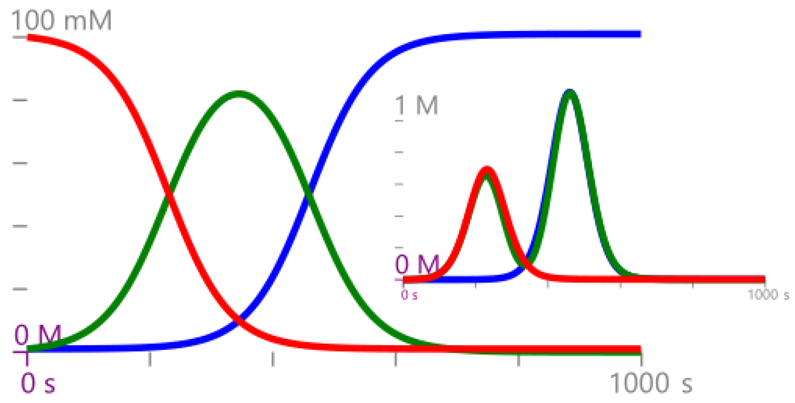
Example 1. Consider the CRN , where . Equivalently, can be expressed as Consider an initial condition of , then the time evolution of mean and variance for the GP defined in Definition 4 are reported in Figure 2. 2.3. Gaussian Semantics for Protocols
There are two possible approaches to a Gaussian semantics of protocols, that is, to a semantics characterized by keeping track of mean and variance of sample concentrations. They differ in the interpretation of the source of noise that produces the variances. We discuss the two options, and then choose one of the two based on both semantic simplicity and relevance to the well-mixed-solution assumption of chemical kinetics.
The first approach we call extrinsic noise. The protocol operations are deterministic, and the the evolution of each sample is also deterministic according to the rate equation (that is, Definition 4 (1)). Here, we imagine running the protocol multiple times over a distribution of initial conditions (i.e., the noise is given extrinsically to the evolution). The outcome is a final distribution that is determined uniquely by the initial distribution and by the deterministic evolution of each run. For example, the sample-split operation here is interpreted as follows. In each run, we have a sample whose concentration in general differs from its mean concentration over all runs. The two parts of a split are assigned identical concentration, which again may differ from the mean concentration. Hence, over all runs, the two parts of the split have identical variance, and their distributions are perfectly correlated, having the same concentration in each run. The subsequent time evolution of the two parts of the split is deterministic and hence identical (for, say, a split). In summary, in the extrinsic noise approach, the variance on the trajectories is due to the distribution of deterministic trajectories for the different initial conditions.
The second approach we call intrinsic noise. The protocol operations are again deterministic, but the evolution in each separate sample is driven by the Chemical Master Equation (i.e., the noise is intrinsic to the evolution). Here, we imagine running the protocol many times on the same initial conditions, and the variance of each sample is due ultimately to random thermal noise in each run. This model assumes a Markovian evolution of the underlying stochastic system, implying that no two events may happen at the same time (even in separate samples). Furthermore, as usual, we assume that chemical solutions are well-mixed: the probability of a reaction (a molecular collision) is independent of the initial position of the molecules in the solution. Moreover, the well-mixture of solutions is driven by uncorrelated thermal noise in separate samples. Given two initially identical but separate samples, the first chemical reaction in each sample (the first “fruitful” collision that follows a usually large number of mixing collisions) is determined by uncorrelated random processes, and their first reaction cannot happen at exactly the same time. Therefore, in contrast to the extrinsic noise approach, a sample-split operation results in two samples that are completely uncorrelated, at least on the time scale of the first chemical reaction in each sample. In summary, in the intrinsic noise approach, the variance on the trajectories is due to the distribution of stochastic trajectories for identical initial conditions.
In both approaches, the variance computations for mix and for split are the same: mix uses the squared-coefficient law to determine the variance of two mixed samples, while split does not change the variance of the sample being split. The only practical difference is that in the intrinsic noise interpretation we do not need to keep track of the correlation between different samples: we take it to be always zero in view of the well-mixed-solution assumption. As a consequence, each sample needs to keep track of its internal correlations represented as a local matrix of size , but not of its correlations with other samples, which would require a larger global matrix of potentially unbounded size. Therefore, the intrinsic noise interpretation results in a vast simplification of the semantics (Definition 6) that does not require keeping track of correlations of concentrations across separate samples. In the rest of the paper, we consider only the intrinsic noise semantics.
Definition 6 (Gaussian Semantics of a Protocol—Intrinsic Noise).
The intrinsic-noise Gaussian semantics of a protocol for a CRN , under environment , for a fixed horizon H with no ill-posed time evolutions, denotes the final CRN state (Definition 2) of the protocol and is defined inductively as follows: together with defined as:The semantics of derives from Definition 4. The substitution notation represents a function that is identical to ρ except that at x it yields v; this may be extended to the case where x is a vector of distinct variables and v is a vector of equal size. The variables introduced by are used linearly (i.e., must occur exactly once in their scope), implying that each sample is consumed whenever used.
We say that the components of a CRN state form a Gaussian state, and sometimes we say that the protocol semantics produces a Gaussian state (as part of a CRN state).
The semantics of Definition 6 combines the end states of sub-protocols by linear operators, as we show in the examples below. We stress that it does not, however, provide a time-domain GP: just the protocol end state as a Gaussian state (random variable). In particular, a protocol like introduces a discontinuity at the end time p, where all the concentrations go to zero; other discontinuities can be introduced by . A protocol may have a finite number of such discontinuities corresponding to liquid handling operations, and otherwise proceeds by LNA-derived GPs and by linear combinations of Gaussian states at the discontinuity points.
It is instructive to interpret our protocol operators as linear operators on Gaussian states: this justifies how covariance matrices are handled in Definition 6, and it easily leads to a generalized class of possible protocol operators. We discuss linear protocol operators in the examples below.
Example 2. The operator combines the concentrations, covariances, and temperatures of the two input samples proportionally to their volumes. The resulting covariance matrix, in particular, can be justified as follows. Consider two (input) states with and . Let 0 and 1 denote null and identity vectors and matrices of size k and . Consider a third null state , with and . The joint Gaussian distribution of is given by Define the symmetric hollow linear operator The zeros on the diagonal (hollowness) imply that the inputs states are zeroed after the operation, and hence discarded. Applying this operator to the joint distribution, by the linear combination of normal random variables we obtain a new Gaussian distribution with: Hence, all is left of is the output state where and as in Definition 6.
Example 3. The operator splits a sample in two parts, preserving the concentration and consequently the covariance of the input sample. The resulting covariance matrix, in particular, can be justified as follows. Consider one (input) state and two null states , with . As above, consider the joint distribution of these three states, and define the symmetric hollow linear operator The 1s imply that concentrations are not affected. The whole submatrix of output states being zero implies that any initial values of output states are ignored. Applying this operator to the joint distribution, we obtain: By projecting on B and C, we are left with the two output states , , as in Definition 6. The correlation between B and C that is present in is not reflected in these outcomes: it is discarded on the basis of the well-mixed-solution assumption.
Example 4. In general, any symmetric hollow linear operator, where the submatrix of the intended output states is also zero, describes a possible protocol operation over samples. As a further example, consider a different splitting operator, , that intuitively works as follows. A membrane permeable only to water is placed in the middle of an input sample , initially producing two samples of volume , but with unchanged concentrations. Then, an osmotic pressure is introduced (by some mechanism) that causes a proportion of the water (and volume) to move from one side to the other, but without transferring any other molecules. As the volumes change, the concentrations increase in one part and decrease in the other. Consider, as in , two initial null states B and C and the joint distributions of those three states . Define a symmetric linear operator Applying this operator to the joint distribution we obtain:producing the two output states and describing the situation after the osmotic pressure is applied. Again, we discard the correlation between B and C that is present in on the basis of the well-mixed-solution assumption. Example 5. We compute the validity of some simple equivalences between protocols by applying the Gaussian Semantics to both sides of the equivalence. Consider the CRN state over a single species having mean (a singleton vector) and variance (a matrix). This CRN state can be produced by a specific CRN [19], but here we add it as a new primitive protocol and extend our semantics to include . Note first that mixing two uncorrelated Poisson states does not yield a Poisson state (the variance changes to ). Then, the following equation holds: That is, in the intrinsic-noise semantics, mixing two correlated (by Split) Poisson states is the same as mixing two uncorrelated Poisson states, because of the implicit decorrelation that happens at each . An alternative semantics that would take into account a correlation due to could instead possibly satisfy the appealing equation for any P (i.e., splitting and remixing makes no change), but this does not hold in our semantics for , where the left hand side yields (i.e., splitting, decorrelating, and remixing makes a change).
The operator can be understood as diluting the two input samples into the resulting larger output volume. We can similarly consider a operator that operates on a single sample, and we can even generalize it to concentrate a sample into a smaller volume. In either case, let W be a new forced volume, and U be a new forced temperature for the sample. Let us define where . Then, the following equation holds: Note that, by diluting to a fixed new volume W, we obtain a protocol equivalence that does not mention, in the equivalence itself, the volumes resulting from the sub-protocols (which of course occur in the semantics). If instead we diluted by a factor (e.g., factor = 2 to multiply volume by 2), then it would seem necessary to refer to the in the equivalence.
To end this section, we provide an extension of syntax and semantics for the optimization of protocols. An optimize protocol directive identifies a vector of variables within a protocol to be varied in order to minimize an arbitrary cost function that is a function of those variables and of a collection of initial values. The semantics can be given concisely but implicitly in terms of an function: a specific realization of this construct is then the subject of the next section.
Definition 7 (Gaussian Semantics of a Protocol—Optimization).
Let be a vector of (optimization) variables, and be a vector of (initialization) variables with (initial values) , where all the variables are distinct and is disjoint from . Let be a protocol for a CRN , with free variables z and k and with any other free variables covered by an environment . Given a cost function , and a dataset , the instruction “optimize k=r, z in P with C given " provides a vector in of optimized values for the z variables (For simplicity, we omit extending the syntax with new representations for C and , and we let them represent themselves). The optimization is based on a stochastic process derived from P via Definition 6.where stands for the expectation with respect the conditional distribution of given . From Definition 6, it follows that, for any
is a Gaussian random variable. In what follows, for the purpose of optimization, we further assume that
is a Gaussian process defined on the sample space
, i.e., that for any possible
and
and
are jointly Gaussian. Such an assumption is standard [
6] and natural for our setting (e.g., it is guaranteed to hold for different equilibration times) and guarantees that we can optimize protocols by employing results from Gaussian process optimization as described in detail in
Section 2.4.
2.4. Optimization of Protocols through Gaussian Process Regression
In Definition 7 we introduced the syntax and semantics for the optimization of a protocol from data. In this section, we show how the optimization variables can be selected in practice. In particular, we leverage existing results for Gaussian processes (GPs) [
6]. We start by considering the dataset
comprising
executions of the protocol for possibly different initial conditions, i.e., each entry gives the concentration of the species after the execution of the protocol
, where the protocol has been run with
. Then, we can predict the output of the protocol starting from
by computing the conditional distribution of
(Gaussian process introduced in Definition 7) given the data in
. In particular, under the assumption that
is Gaussian, it is well known that the resulting posterior model,
, is still Gaussian with mean and covariance functions given by
where
is a diagonal covariance modeling i.i.d. Gaussian observation noise with variance
,
and
are the prior mean and covariance functions,
is the covariance between
and all the points in
, and
,
are vectors of dimensions
containing for all
, respectively,
and
[
6]. Note that, in order to encode our prior information of the protocol, we take
to be the mean of the GP as defined in Definition 6, while for the variance we can have
to be any standard kernel [
6]; in the experiments, as is standard in the literature, we consider the widely used squared exponential kernel, which is expressive enough to approximate any continuous function arbitrarily well [
20]. However, we remark that, for any parametric kernel, such as the squared exponential, we can still select the hyper-parameters that best fit the variance given by Definition 6 as well as the data [
6]. We should also stress that the resulting
is a Gaussian process that merges in a principled way (i.e., via Bayes’ rule) our prior knowledge of the model (given by Definition 6) with the new information given in
Furthermore, it is worth stressing again that
is a GP with input space given by
which is substantially different from the GP defined by the LNA (Definition 5), where the GP was defined over time.
For a given set of initialization parameters
r our goal is to synthesize the optimization variables that optimize the protocol with respect to a given cost specification
, i.e., we want to find
such that
where
is the expectation with respect to the GP given by Equations (
3) and (
4)). Note that
r is a known vector of reals (see Definition 7), hence we only need to optimize for the free parameters
u. In general, the computation of
in Equation (
5) requires solving a non-convex optimization problem that cannot be solved exactly [
21]. In this paper, we approximate Equation (
5) via gradient-based methods. These methods, such as gradient descent, require the computation of the gradient of the expectation of
C with respect to
u:
Unfortunately, direct computation of the gradient in (
6) is infeasible in general, as the probability distribution where the expectation is taken depends on
u itself (note that
). However, for the GP case, as shown in Lemma 1, the gradient of interest can be computed directly by reparametrizing the Gaussian distribution induced by Equations (
3) and (
4).
Lemma 1. For , let be the matrix such that . Then, it holds that In particular, as defined above is guaranteed to exist under the assumption that is positive definite and can be computed via Cholesky decomposition. Furthermore, note that if the output is uni-dimensional, then is simply the standard deviation of the posterior GP in .
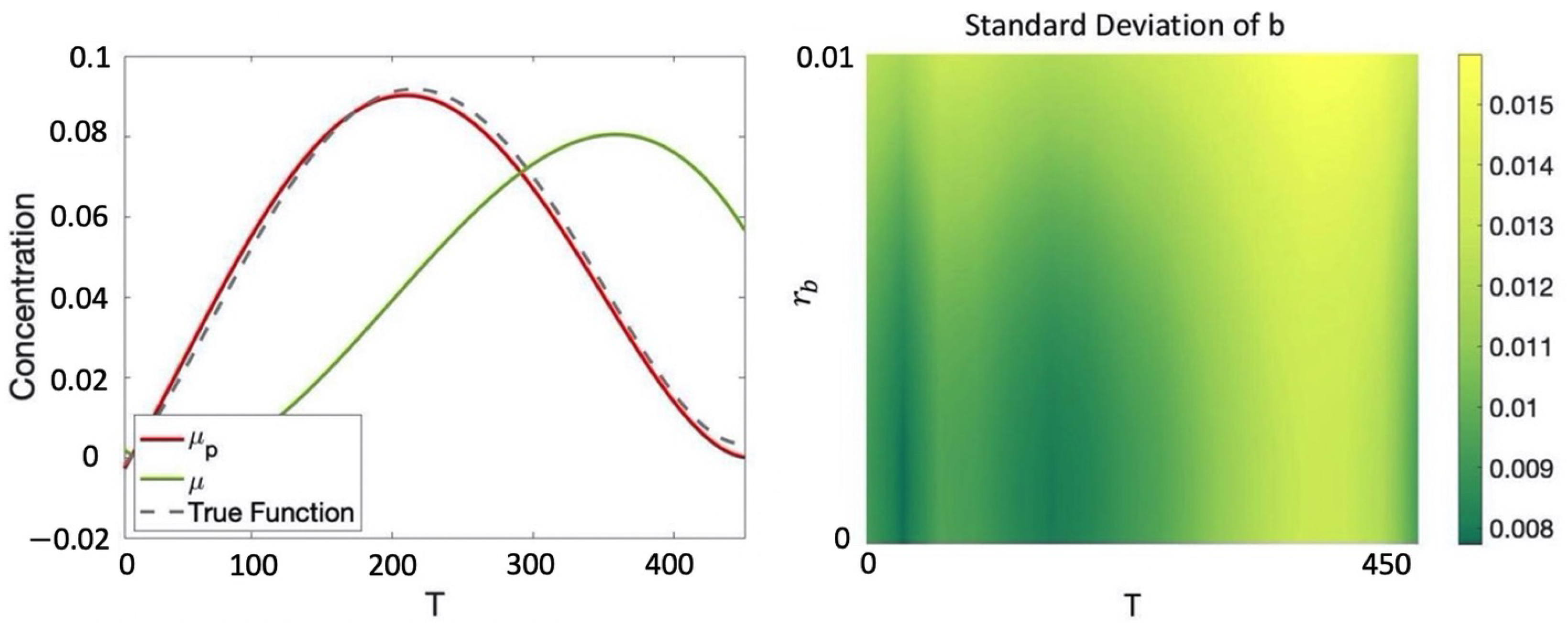
Example 6. Given the CRN introduced in Example 1, consider the protocolwhich seeks to evolve the various species from an initial starting concentration of mM for species a and mM for both species b and c for T seconds. Hence, for this example, we have including initial conditions, volume, and temperature and , that is, the only optimization variable is the equilibration time. We consider a dataset composed of the following six data points (for simplicity we report the output values of only species b and omit unit of measurement, which are mM for concentration, μL for volume, Celsius degrees for temperature, and seconds for equilibration time):where, for example, in we have that the initial concentration for are, respectively, , , , volume and temperature at which the experiment is performed are 1 and 20 and the observed value for b at the end of the protocol for is We assume an additive Gaussian observation noise (noise in the collection of the data) with standard deviation . Note that the initial conditions of the protocol in the various data points in general differ from those of P, which motivates having Equations (3) and (4) dependent on both r and u. We consider the prior mean given by Equation (1) and independent squared exponential kernels for each species with hyper-parameters optimized through maximum likelihood estimation (MLE) [6]. The resulting posterior GP is reported in Figure 3, where is compared with the prior mean and the true underlying dynamics for species b (assumed for this example to be deterministic). We note that with just 6 data points in , the posterior GP is able to correctly recover the true behavior of b with relatively low uncertainty. We would like to maximize the concentration of b after the execution of the protocol. This can be easily encoded with the following cost function: For , the value obtained is , which is simply the one that maximizes the posterior mean. In Section 3.1, we will show how, for more complex specifications, the optimization process will become more challenging because of the need to also account for the variance in order to balance between exploration and exploitation. 

