A Skyline-Based Decision Boundary Estimation Method for Binominal Classification in Big Data

Abstract

One of the most common tasks nowadays in big data environments is the need to classify large amounts of data. There are numerous classification models designed to perform best in different environments and datasets, each with its advantages and disadvantages. However, when dealing with big data, their performance is significantly degraded because they are not designed—or even capable—of handling very large datasets. The current approach is based on a novel proposal of exploiting the dynamics of skyline queries to efficiently identify the decision boundary and classify big data. A comparison against the popular k-nearest neighbor (k-NN), support vector machines (SVM) and naïve Bayes classification algorithms shows that the proposed method is faster than the k-NN and the SVM. The novelty of this method is based on the fact that only a small number of computations are needed in order to make a prediction, while its full potential is revealed in very large datasets.

1. Introduction

The increased amount of high-volume, high-velocity, high-variety and high-veracity data produced in the last decade has created the need to develop cost-effective techniques to manage them, which fall under the term big data [1]. Today, a considerably large percent of data is generated by social media and e-commerce, which will change with the rise of the Internet of things (IoT). Devices will take the lead—and with the expanding rate of billions to trillions of devices in the next years—the amount of generated data will be massive. In many cases, such enormous volumes of data need to be stored for further analysis, or even processed on the fly to reveal meaningful insights.

Nevertheless, continuously retrieving and storing large amounts of data that may be inaccurate, incomplete or unlabeled may eventually decrease their quality and eventually their value [2]. On top of this, storage costs will increased as data piles up. Thus, at this point, the term “smart data” starts to appear in the literature [3,4], which refers to the transformation of data with data-mining or machine-learning (ML) techniques, in order to reduce the processing cost imposed by their volume, but with a primary goal of maintaining their real value.

To deal with the problems imposed by the volume, one may consider the reduction of cardinality—or dimensionality—of the data for which various methods have been proposed. Such a problem occurs with the R-trees [5] when the space has more than 4–5 dimensions—named as the curse of dimensionality. The simplest case of volume reduction can be achieved by sampling techniques [6] that directly reduce the cardinality of the dataset. The dimensionality reduction approach can be performed either through feature elimination, extraction or selection techniques [7,8], or by directly mapping a multi-dimension dataset to a lower dimensionality space. The last approach can be performed with statistical data mining such as principle component analysis (PCA) [9], stochastic approaches such as t- distributed stochastic neighbor embedding (t-SNE) [10] or neural network approaches such as auto encoders [11].

Dimensionality reduction techniques are commonly used to improve the performance of a classifier. However, ML methods have reached a point at which we can combine even a set of weak classifiers using ensemble learning techniques [12] to produce good results. With this in mind, each time a new classifier is proposed, questions arise if we really need one more [13].

Even with these techniques, it is not always feasible to perform a classification task with low processing costs in a big data environment, since traditional classification algorithms are designed primarily to achieve exceptional accuracy with tradeoffs between space or time complexity. In a k-nearest neighbor (K-NN) classifier, the main cost reflects to the cost of computing the distances from every element, in naïve Bayes to compute a large number of conditional probabilities, in probabilistic neural networks (PNN) or its radial basis function (RBF) alternative to sum local decision functions and in support vector machine (SVM) to compute complex hyperplane equations.

In this work—which is an extension of the work in [14]—we propose a straightforward method for classification which is significantly more efficient than traditional classification algorithms in big data environments. The proposed method uses skyline queries to identify boundary points and construct final decision boundaries. Primarily skyline queries were designed to identify the most preferable options based on certain, sometimes contradicting, optimization criteria. Skyline queries are categorized as a dominance-based multiobjective optimization approach that was developed under the scope that the dataset in use does not entirely fit in memory. The multiobjective optimization problem of efficiently identifying the skyline points has its root in the Pareto optimality problem (V. Pareto 1906) which was used in aerospace for aerodynamic shape optimization [15] and in economics for optimal investment portfolio [16]. In computational geometry, the problem is equivalent to the maximal vector problem [17].

To our knowledge, this is the first work that tries to harvest the power of skyline queries in a classification process for big data. The benefits of using such an approach are:

• Even in a very large dataset, decision boundaries are described by a small number of points; thus, a classification process needs to perform only a small number of computations in order to infer the correct class;
• Decision boundaries can be independently computed, allowing for full parallelization of the whole modeling process;
• It is applicable in a wide range of multidimensional environments and specifically in any environment that its dataspace has an ordering, a feature that is inherited from the skyline query family;
• The model can be easily explained and visualized allowing for greater interpretability;
• The decision boundaries can be easily transferred, reused and easily re-optimized allowing Transfer Learning.

In the following, Section 2 briefly summarizes work on skyline queries, Section 3 outlines the preliminary notions and concepts, Section 4 describes the proposed method and its variations, Section 5 outlines the experimental results, Section 6 discusses some possible opportunities and Section 7 concludes.

2. Background and Related Work

We assume that the fundamental data mining and machine-learning methods [9] are extensively and analytically covered in the literature and thus we omit them. The skyline query family [18] is a wide area of research with many applications. Through this section we will highlight the core parts of skyline queries and their applications, particularly with regards to big data-related issues.

2.1. Skyline Query Family

Skyline queries were first introduced in [19]. Their evolution produced indexed and non-index-based methods. The most common index-based method is the branch and bound skyline (BBS) algorithm [20] which uses the R-tree. For the non-indexed approaches, the simplest is the Block Nested-Loop (BNL) algorithm [19], while more sophisticated methods are the Sort-Filter skyline (SFS) algorithm [21] and the linear estimation sort for skyline (LESS) algorithm [17].

There are many different variations of skyline queries trying to solve different problems. For example, ε-skyline [22] allows users to control the number of output skyline points relaxing or restricting the dominance property, k-skyband queries [20] consider that multiple dominated points may be an option, angle-based approach [23] computes the skyline by modifying the dominance property, in [24] authors try to find an approximation of the original skyline, metric skyline [25] is useful to find the strongest DNA sequence similarity where a string is of a more appropriate value representation than a vector, in Euclidean space and [26] studies the cardinality and complexity of skyline queries in anti-correlated distributions. For the cases where the set of skyline points is too large, the representative skyline was proposed [27]. The probabilistic nature of a skyline due to the uncertainty of data that can be described through a probability density function (PDF) is discussed in [28]. Sample-based approaches for skyline cardinality estimation were discussed in [29] while kernel-based in [30]. At this point, it is worth mentioning that the problem of multiobjective optimization using evolutionary algorithms (EA) was studied in the late 90’s with the bright example of the Non-dominated sorting genetic algorithm-II (NSGA-II) algorithm [31] and skyline queries [19] in the early 2000’s.

2.2. Applications of Skyline Queries

There is a wide variety of applications in different environments. In [32,33], authors use skyline queries to efficiently identify the best web services. In [34], authors used a neural network to reduce the search space and efficiently identify skyline candidates which was applied in Bioinformatics [35]. The new cognitive problem of serendipitous discovery [36], which summarizes to the concept of “unexpectantly finding surprisingly interesting points”, was studied in [37], which deals with cell discovery using continuous skyline queries like [38]. This is based on the notion of a dominance graph [38], but it is applied in a different temporal environment.

2.3. Big Data

An extended list of studies about skyline in Hadoop and other index-enable big data systems can be found in [39]. In [40], authors discuss topics on machine learning with big data. A large number of frameworks [41] were developed to handle big data through the use of ML techniques. Several of these techniques are discussed in [2].

3. Preliminaries

This section will discuss the fundamental notions related to this work such as the skyline operator, issues related to its cardinality, dimensionality and time complexity. We will study the 2-dimensional case for simplicity and visualization reasons, but it is evident that it can be extended to more dimensions.

3.1. Skyline Query Family

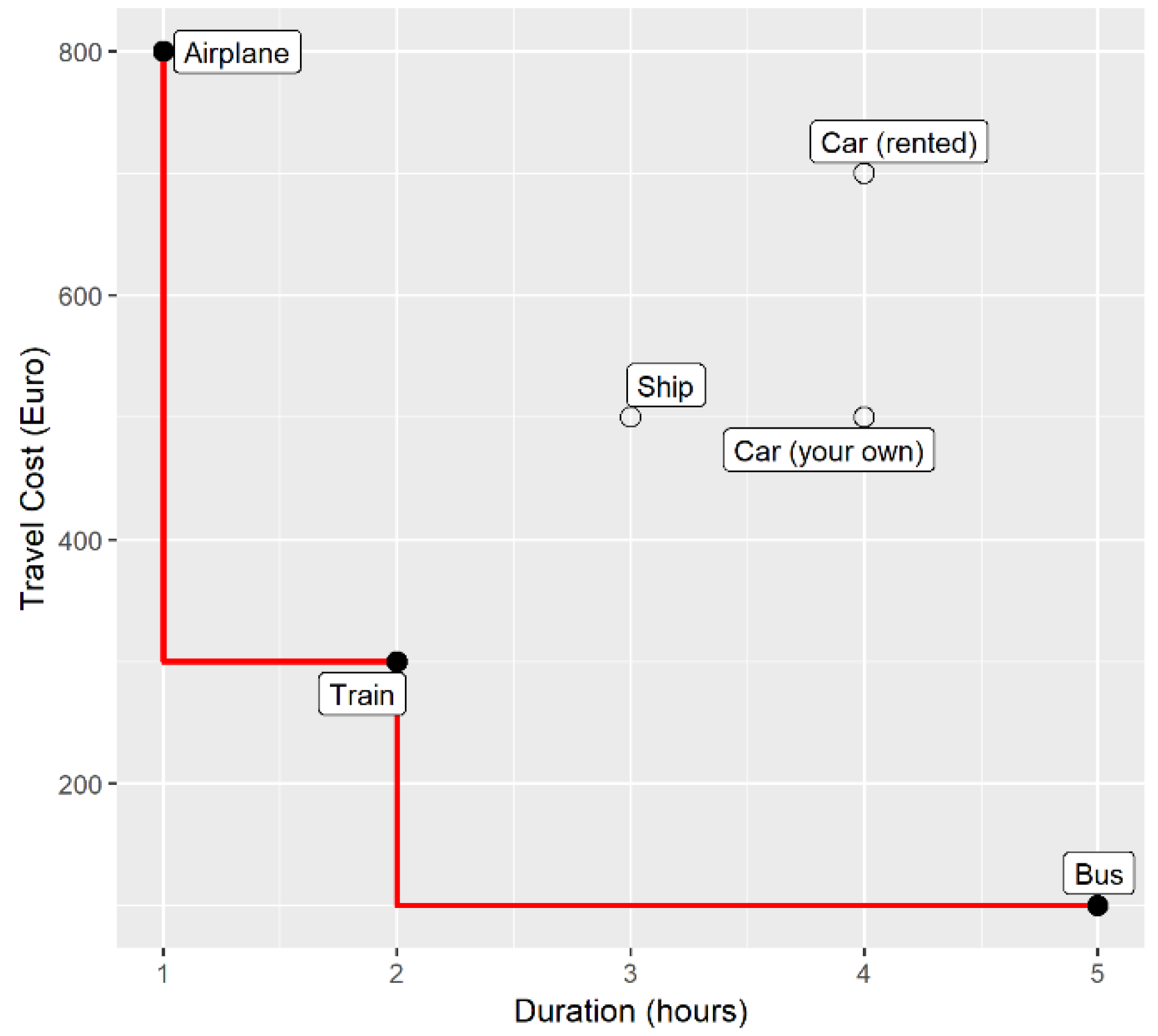
In order to make clear how skyline queries work, we start with an example. Let us assume that we want to go for a trip, and we are trying to find a way towards our destination. The transportation means are quite a lot and each one of them has a different fare. Our preferences suggest that we would like to go by train rather than by airplane in order to enjoy the view. On the other hand, we are going to a business meeting and would feel relaxed if we could get there one day earlier. It is a tough choice, but between our two contradicting criteria (preferences), maximizing the joy (ranked from 1 to 10) of a trip and minimizing the amount of travel time, we will choose the second one (feature selection). We also have another concern. This meeting involves a job interview and thus, we must pay for all the expenses of our trip, making the cost the second criterion in choosing the transportation means. Based on our criteria, we made a research to gather the information about the cost of each transportation means and the time that it needs. We wrote down our results in

Table 1. Dataset of travel options.

Transportation Mean	Time	Cost	Joy
Train	2	300	10
Car (own)	4	500	4
Car (rented)	4	700	4
Ship	3	500	1
Airplane	1	800	8
Bus	5	100	6

(the values may not reflect reality) for better understanding and for completeness we filled in the joy that we would get from the specific transportation means, as we ranked it.

The skyline query solves a multiobjective optimization problem which allows only the survival of the fittest records. The core notion that encompasses is the one of dominance. Only the dominant records can belong to the skyline. A record is said to dominate another record if it is better than this in at least one dimension (feature). A skyline set of points is the set of points that are not dominated by any other point in the dataset. For space considerations we omit the formal definition of dominance and skyline set since it can be found in numerous studies such as in [42].

After the brief introduction of what a skyline is, we can identify that traveling in a rented car is not a good option, since for the same time we can travel in our car with less expenses. The same applies to traveling by ship, in which case, the expenses are the same, but the time it takes is less. By plotting our data and drawing the skyline this becomes clear Figure 1. Traveling by airplane, train or bus belongs to the skyline set and we can choose which one fits best to our needs with tradeoff between time and expenses.

3.2. Cardinality, Distribution and Curse of Dimensionality

The amount of points returned by the skyline drew the attention of researchers [29,30]. The first attempt to estimate the cardinality of the skyline operator was in [43]. Those studies showed that cardinality depends on the distribution of the dataset. For example, anti-correlated distributions, in the case where minimization of preferences is desired, will produce more points than in a normal distribution and thus approaches such as [27] may be preferable. In correlated distributions, the opposite happens. The formula to calculate the number of skyline points in a normal distribution can be found in [30] and is

$$\mathsf{\theta }\left({\left(\ln \mathrm{n}\right)}^{\mathrm{d}-1}/\left(\mathrm{d}-1\right)!\right),$$

(1)

where n is the cardinality of the dataset, d its dimensionality and $\mathsf{\theta }$ denotes the average case scenario. One of the most important factors that determines the cardinality of the skyline is the distribution of the dataset. The second one is dimensionality. The problems that arise due to high dimensional datasets, such as sparse data and high computational cost, were characterized as the “curse of dimensionality” [44] and was first discussed by Bellman [45]. As the dimensionality of space increases, the number of skyline points returned increases too, as presented in Figure 2 for the Gaussian distribution, making the skyline computation on spaces with more than 5-dimensions inefficient.

Nevertheless, there are lot of techniques that reduce the dimensionality of a dataset by simultaneously retaining the core properties of the dataset. The potential of t-SNE [10] and PCA [9] for the visualization of the genomics and MNIST datasets can be seen in [10]. Thus, with these sophisticated methods, PCA for dense data, (truncated singular value decomposition) TruncatedSVD [46] for spare data, t-SNE for small data and the newly developed auto-encoders [11], the high-dimensional data are better confronted.

3.3. Time Complexity

There is a wide variety of algorithms for skyline computation in a wide range of environments. Each algorithm has a different complexity and specific requirements. For example, the most general non-index-based algorithm is the BNL, which is characterized by its simplicity, while the SFS [21] require a sorted normalized dataset. The worst-case time complexity for BNL [19] and LESS [17] is $O\left(k{n}^2\right)$ and for the best case $O\left(kn\right)$, where k denotes the number of dimensions [47].

4. Methodology

As described in the previous section, there exist numerous variations and different factors on how the skyline queries can be applied on a set of data in order to extract the decision boundaries. Since this is a novel and naïve approach based on skyline search, it can be further improved and expanded. The proposed method does not rely on any specific skyline algorithms or index. To retrieve the skyline set, the BNL algorithm was chosen for its simplicity, but any other algorithm can be used. This way, the proposed method computes one skyline for each class which will eventually be part of the decision boundary construction process.

In an abstract approach, the proposed method has one preprocessing task and three normal tasks as follows:

• Define origin points;
• Identify skyline points;
• Construct decision boundaries;
• Perform classification process

The preprocessing task deals with identifying the origin points (preferences) for which each one of the skyline queries will be performed. The first task computes the skyline based on the preferences set by the preprocessing task. The second task determines the boundaries based on the points returned by the skyline and the third one performs the classification task. Through our research we identified four different approaches on how to compute the skyline set and three different approaches on how to compute the boundaries. By using different skyline identification approaches we study how our method behaves when we retrieve a broader set of skyline points and if this assists in the estimation of the decision boundaries. Through the rest of this paper, we assume that the datasets consists of two classes (since the proposed method is binominal). As our proposed method performs best in big data environments, we targeted on a synthetic dataset of 1 M points randomly generated in space, following the Gaussian distribution. From a wide number of real datasets, we focused on a dataset that has at least 10,000 records. We note that the skyline computation is independent from the underlying distribution.

4.1. Define the Origin Points

In order to compute the skyline set from a dataset, first we must define the preferences. It is common in literature, if not mentioned, that the minimization of preferences is desired. In our case, since we have a binominal classifier, which classifies an object between two classes, we must compute two skylines and thus we must define two origin points. In a 2-dimensional space, we have four options as preferences based on the combination of minimizing or maximizing each dimension. Each one of these points depicts one of the corners of the dataspace. Thus, in the preprocessing, we manually select which corner of the dataspace we would like to be the origin for each class, and thus, each skyline that we need to compute. This process could have been automated by taking into account the location of classes in space. Nevertheless, there should be a different approach for each case in the skyline retrieval that will be described in the following subsection. Note that the origin points that are assigned to each class are never on the same corner of dataspace. Moreover, in a 2^d space there are four corner points and, in a d-dimensional space the number of required points is $2^d$. Thus, for every experiment we need to perform $2^d$ skyline queries. The curse of dimensionality is a common issue in r-trees and skyline queries.

4.2. Identifying Skyline Points

Having defined the origin points, we can now compute the skyline for each class. This phase is completely independent for each class and thus we can parallelize the whole process. Additionally, skyline queries over Hadoop MapReduce are extendedly studied, making our method compatible with MapReduce. To accomplish this process, we studied different approaches on how we could perform one or more skyline queries in order to get a set of points that best describes a decision boundary.

Among those cases there are the single skyline which performs a single skyline for each class, the double skyline, similar to the single skyline, but it computes two skylines for each class, the opposite skyline, which tries to retrieve the skyline points that reside in two opposites sides of each class and the smart skyline which takes into account the relative location of the two classes of the dataset. Each approach has its benefits, like better accuracy, computation time and boundary approximation, but this comes to the expense of computation due to multiple skyline queries.

As previously mentioned, we use the BNL algorithm for skyline computation which has $O\left(k{n}^2\right)$ complexity. Thus, the complexity of identifying the points that will assist in estimating the decision boundaries is $2\ast O\left(k{n}^2\right)$, where k is the number of dimensions and n the cardinality of each class. Below we present in detail the four different approaches for skyline computation:

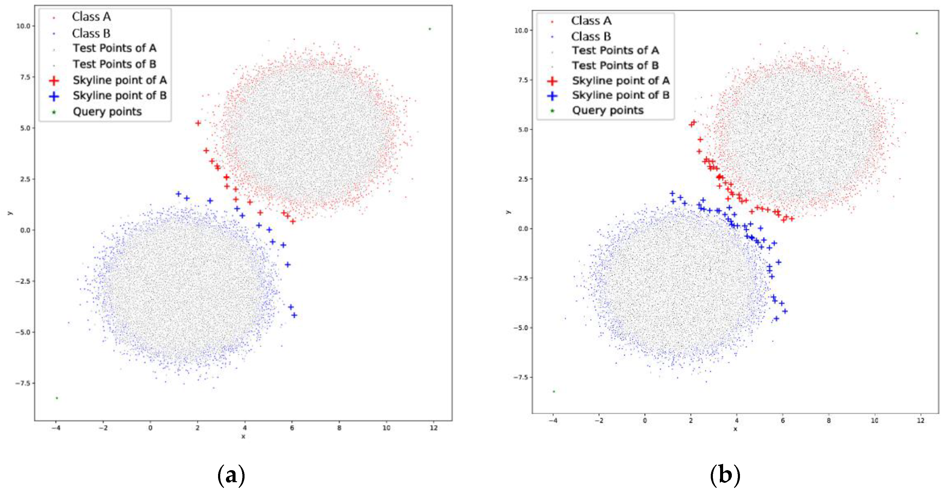
• single skyline: In this option, we define the origin points and perform a single skyline for each cluster, as depicted in Figure 3a. This approach performs better in dense data as the boundaries can be straightforwardly defined. This is the simplest case with the minimum computation cost as 2 * O(kn²).
• double skyline: This case, as seen in Figure 3b is similar to the one above, but it computes two skylines for each cluster using the same origins. The process computes the first skyline, removes the points from the initial dataset, but stores them in a list and then performs the second skyline computation. Then, it merges the points from the two skylines. This is done for both Cluster A and Cluster B and when completed, it proceeds to the next phase. This approach may have additional overhead as 4 * O(kn²), but the resulted boundaries are more accurate in sparse data.
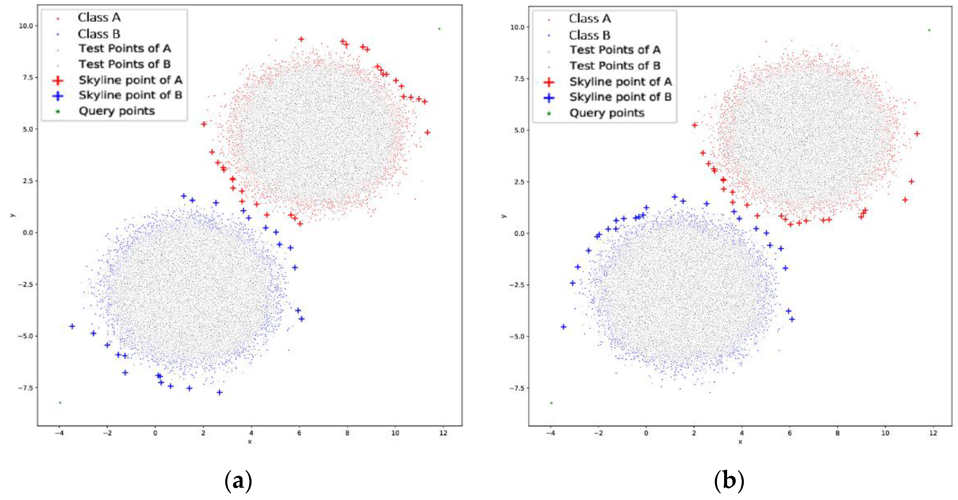
• opposite skyline: The opposite skyline, depicted in Figure 4a tries to retrieve the skyline points that reside in two opposite sides of each cluster. In this way, we try to enclose the area where the data on each cluster are. Even though this approach may not be desirable in many cases, it has very good results even in overlapping clusters, but it has increased overhead as 4 * O(kn²). An exception to this approach is the need of four origin points, two for each cluster which will be in the opposite side.
• smart skyline: The smart skyline of Figure 4b takes into account the relative location of the two clusters in order to maximize the length of the boundary line. This approach, instead of collecting more points in the same vicinity, such as the double skyline, retrieves points in such a way that it extends the boundary line around the cluster in order to get more chances in dividing them. This method has the same complexity as the double and opposite skyline approach.

Current research on skyline computation over big data employees MapReduce-based skyline query computation approaches and have managed to compute the skyline in up to 10 dimensions and 4B records [39]. In such an extreme case, using a uniform distributed dataset, the number of skyline points would be approximately 3.5 M, based on Equation (1). It is common in skyline query computation that as dimensionality increases, the number of skyline points may become too numerous because the chance of one point to dominate another decreases. Taking this into account, researchers have proposed approaches to control the output size k of a skyline query and retrieve a subset of the original skyline set which holds its properties and maximizes insights. Some of those approaches are the Top-k skyline [20,48], k-representative [27], Distance-based k-representative [49], ε-skyline [22]. In highly demanding datasets where the total number k of skyline points exceeds certain thresholds, the aforementioned proposed skyline variants can be used instead of the BNL for skyline identification.

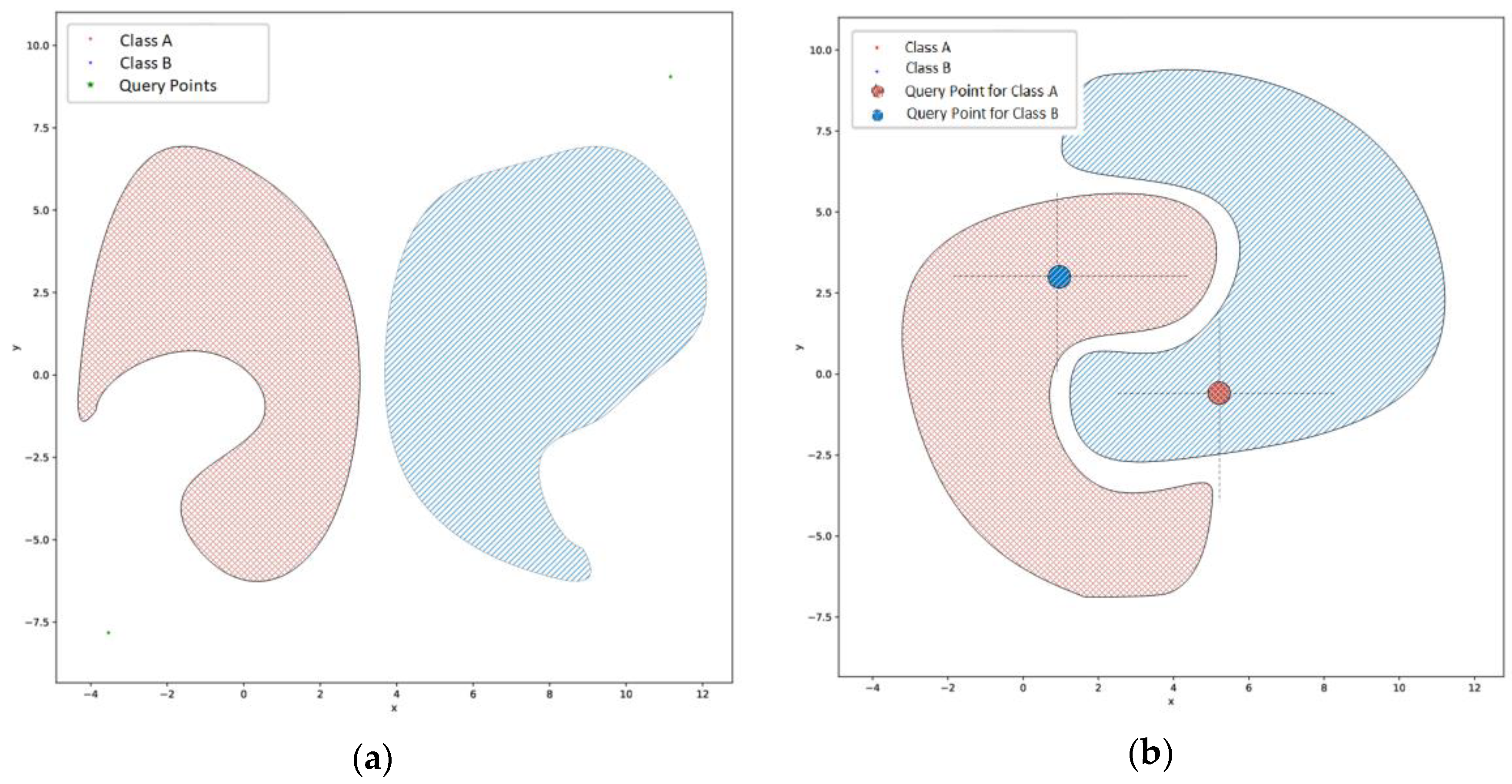
Through our experimentation, we studied the case of large scale convex shaped datasets. Reasoning about nonconvex datasets, our method can be applied in cases like the one presented in Figure 5a following the same steps as described previously in order to define the origin points and retrieve the skyline. In more complex nonconvex datasets like a 2-class banana dataset (Figure 5b) the identification of the skyline is more complex. In this case the two origin points that can be defined to retrieve the skyline for each class are presented in Figure 5b. Moreover, for this case, for each origin/query point two skyline queries should be issued to properly form the decision boundaries. For the case of Class A, the two skyline queries should be issued in the upper left and lower left quadrants. For the case of Class B, the two skyline queries should be issued in the upper right and lower right quadrant. Issuing skyline queries in different quadrants can be performed by setting the appropriate preferences on minimizing or maximizing a dimension. In the case of nonconvex datasets, the variant of constrained skyline queries [20,48] can be found useful in order to form partial boundaries. The case of noncontiguous datasets does not affect the skyline identification process and a single origin point can be used for each class as described in the general case.

4.3. Decision Boundary Construction

The boundary construction process uses the skyline points retrieved in the previous step and uses them to estimate the decision boundaries. The construction process is based on four different approaches as presented below.

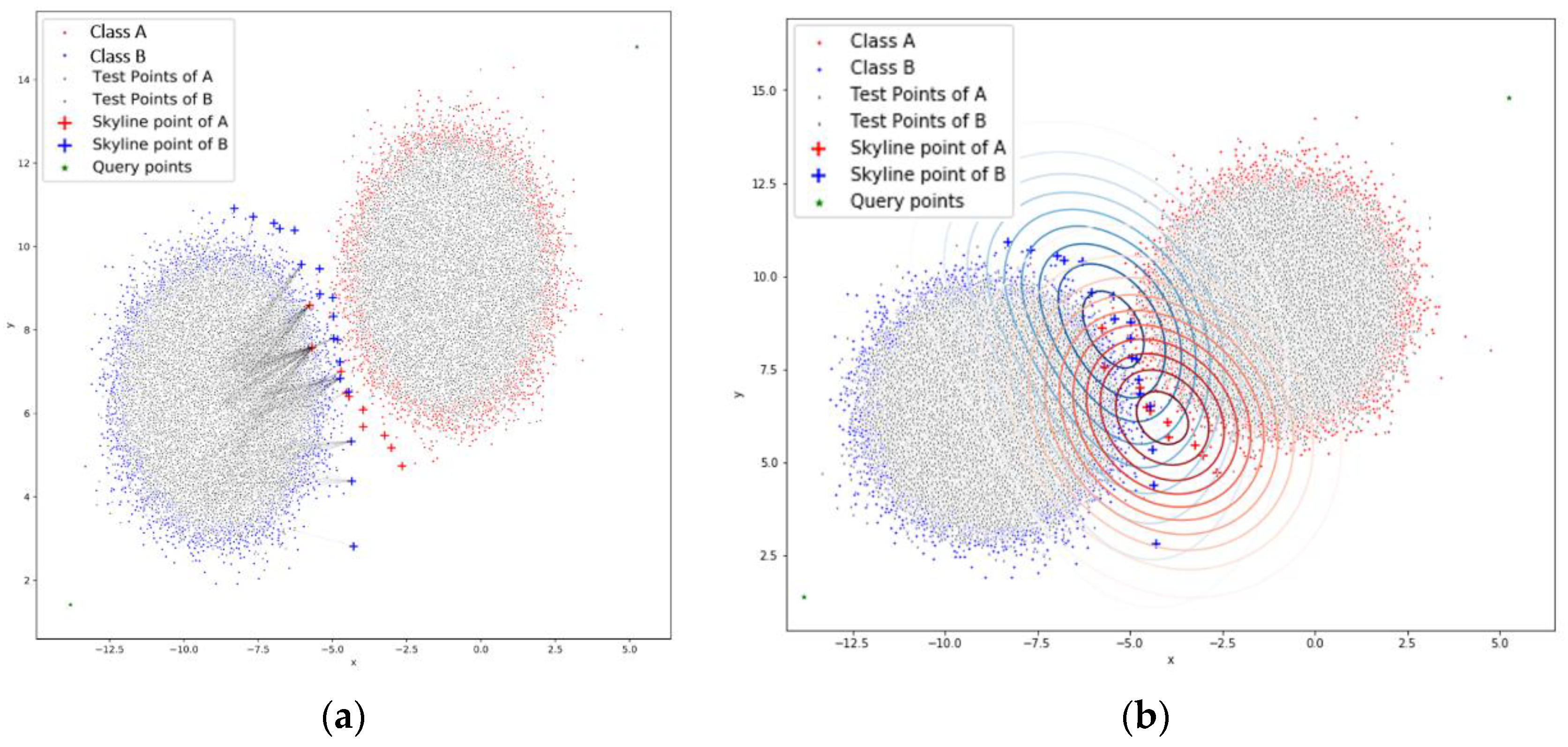
• SKY-nearest neighbor (SKY–NN): This is the simplest case where the decision is made based on the K-NN paradigm (Figure 6a) by retrieving the k nearest skyline points. This method does not make any further computations to produce a boundary, but it uses the skyline points that were retrieved from the previous step as is. This approach is the easiest case to be scaled up in more than two dimensions due to the simplicity and the inherited properties of the K-NN paradigm.
• Parzen-window method: The Parzen approach, visualized in Figure 6b computes the probability that a point belongs to a certain class, based on the set of skyline points. It is a probabilistic approach that estimates a distribution or data points via a linear combination of kernels centered on the observed points of the skyline. We note that in this case only the simple skyline is used and not any variation like the probabilistic skyline.
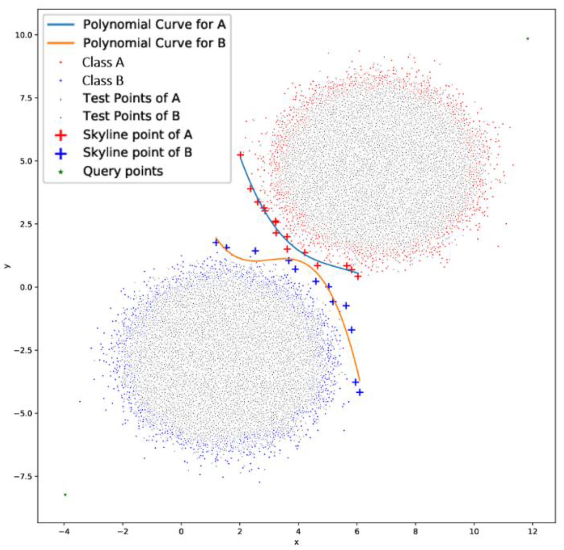
• Dual curve with Polynomial Curve-fitting: In this method, we use a curve-fitting method to compute a curve (polynomial function) Figure 7 that best fits to our data, which in this case, are the skyline points. This case computes two curves, one for each class. A factor of importance is the degree of the polynomial function.
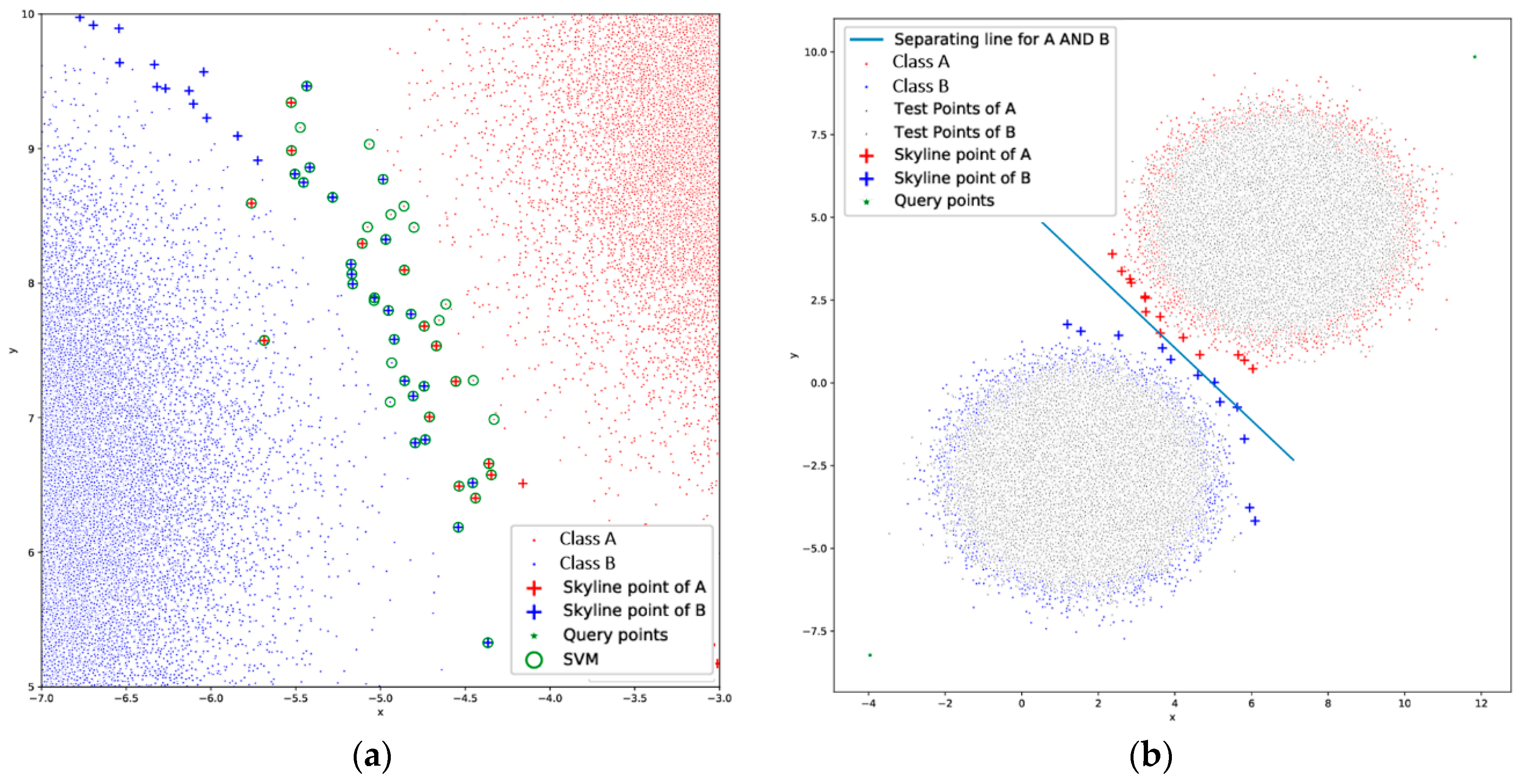
• Single curve with Polynomial Curve-fitting: Throughout our experimental phase, we observed that many and in some cases even all of the skyline points are a subset of the support vectors used by the final SVM (Figure 8a). Based on this observation, this approach uses the skyline points identified from the two classes, to compute one curve or a straight line in the case presented in Figure 8b. This final curve (line) resembles an SVM, but it is different. It can be considered as an approximate vector similar to an SVM that can be easily computed in big data environments.

4.4. Classification Task

After computing the decision boundaries, the classification phase starts. From the previous phase there exist two sets of points or curves that depict to the decision boundaries. During the classification process, for each point we want to classify, we compute its distance from each boundary line, or its probability based on the skyline points. The exact approach is described below.

• SKY-Nearest Neighbor (SKY–NN): From each of the two sets of skyline points we retrieve the k-closest points to the point under consideration. Its class can be defined based on two alternatives, either by majority voting or by computing the total distance of the point under consideration from all the selected points of each class. The set from which the point has the smallest distance determines its class.
• Parzen-window method: This method computes the probability of a point to belong to the one or the other class based on the two sets of skyline points that were retrieved. After computing the probability for the two sets of skyline points, the method assigns the point to the class with the highest probability.
• Dual curve with Polynomial Curve-fitting: In this case, there exist two curves and thus two polynomial functions. Each function receives as input the x-value of the point under consideration. Both functions produce a y-value which is compared to the y-value of the point under consideration. The point will belong to the class where its y-value is closer to the one produced by the polynomial function.
• Single curve with Polynomial Curve-fitting: In this case, we use the skyline points from both classes to produce a single curve and in the simplest case that we examine, a straight line. The function that represents the line receives the x-value of the point under consideration as input. It produces a y-value, which is compared to the y-value of the point. Depending on whether or not the y-value under consideration is greater or smaller than the y-value produced by the function we can infer the class that the point belongs to.

As described and presented with the previous figures, the model can be easily visualized and explained. This gives the user the ability to understand its structure and explain its output reducing the chances to produce a biased algorithm. Moreover, the boundaries can be easily transferred either in the form of a set of points or in a polynomial function and re-optimized easily in a new system if needed. Note that the computation of skylines on each class is independent and thus parallelization can be achieved. Since the proposed method is based on skyline queries, it is applicable in every environment that the skyline queries exist, like the text dataspace, which has an alphanumerical order.

The most important fact is that the skyline queries produce a small number of points, relative to the original dataset thus, the proposed method uses a very small number of points from the original dataset to estimate the boundaries. More precisely, in a 2 M dataset with two balanced classes our approach needs 14 points for each, which equals to 28 points in total. The small number of points needed to define the boundaries consecutively leads to a small number of computations during the identification of the class of a new point.

5. Experiments

This section presents the time needed to perform a classification task and the accuracy of our proposed method. Our intention is to show how this method behaves in close or overlapping clusters since in separable clusters 100% accuracy can be achieved. In our experimentation, we used three synthetic and one real dataset consisting of a large number of points in order to describe how our method behaves in big data environments. Both datasets consist of two balanced classes. The synthetic datasets are randomly generated following a Gaussian distribution, the classes have a varying overlapping factor in order to demonstrate how our method performs and consists of 1 M points in total. The real dataset can be retrieved from [50] and has labeled data that describes if a person is female or male based on their height and weight. It consists of 10,000 points and its classes have a high level of overlap. For a ground truth accuracy on the three datasets, we performed a classification task using python open-source tools for applying the k-NN, naïve Bayes and SVM classifiers. In the case of the SVM classifier we used a linear kernel and a C-value of 1. We selected those classifiers because they resemble the SKY–NN, Parzen and polynomial fit approaches that we follow. The proposed method is implemented in Java SE and all the experiments were performed with an Intel Core i5 with 6 GB RAM.

For the synthetic datasets that consist of 1 M points the naïve Bayes approach finished in less than a second, the SVM took several minutes (

Table 2. Time needed to compute decision boundaries.

	k-NN	Naïve Bayes	SVM
Synthetic Dataset I (in ms)	DNF	918	362,255
Synthetic Dataset II (in ms)	DNF	449	173,397
Synthetic Dataset III (in ms)	DNF	493	175,627
real dataset (in ms)	500	20	1500

with time in milliseconds) and the k-NN did not finish in a reasonable time. This behavior reveals the problems that arise in a classification task due to the large number of computations needed in an environment with a large number of points. In terms of accuracy, both naïve Bayes and SVM achieved 100% accuracy as presented in

Table 3. Accuracy with Python and R framework.

	k-NN	Naïve Bayes	SVM
Synthetic Dataset I (in ms)	DNF	100.00	100.00
Synthetic Dataset II (in ms)	DNF	100.00	100.00
Synthetic Dataset III (in ms)	DNF	100.00	100.00
Real dataset (in ms)	91.13	87.97	92.13

. For the real dataset which consists of 10,000 points all algorithms were able to produce a result in a reasonable time (Table 2 with time in milliseconds). Their accuracy is around 90% (Table 3) since the classes of the dataset have a high degree of overlap.

In Section 4, we discussed about the approaches of retrieving the skyline points in order to construct the boundaries and perform the classification process. Nevertheless, there are many fine-tune approaches on how many or which of the skyline points are needed to be used in the decision process for each point. Retrieving the k-NN skyline points requires $O\left(n\right)$ time and assuming that there are m points to be classified, the total overhead will be $m\ast O\left(n\right)$. The complexity of the polynomial curve-fitting approach depends on the method that is selected.

After we outlined the various approaches that can be followed, we present (

Table 4. Total time needed on average to perform a classification task on the synthetic datasets.

Skyline Mode	SKY–NN	Parzen	Polyn.
Single	2751	3999	12,438
Double	5423	6513	11,306
Opposite	4659	5180	13,048
Smart	4256	5360	15,833

and

Table 5. Total time needed to perform a classification task on the real dataset.

Skyline Mode	SKY–NN	Parzen	Polyn.
Single	57	103.56	89.6
Double	180.9	251.07	225.32
Opposite	117.87	201.65	178.9
Smart	70.16	160.58	105.3

) the total time (in milliseconds) needed to identify the boundaries and perform a classification task, using three skyline points. For the polynomial case, the degree of the function is two. As presented the SKY–NN method is the fastest, while the Parzen performs better in larger datasets and the polynomial approach in smaller ones. Because the SKY–SVM is not applicable with opposite skyline, for continuity, the time and accuracy metrics will be presented at the end of each subsection that follows.

Taking into account the previously mentioned state-of-the-art classifiers, our method is faster than the k-NN and the SVM, but slower than the naïve Bayes. In terms of accuracy, as it will be presented, it achieves remarkable results achieving 100% accuracy in many cases. Those results are achieved at a reasonable time by using a small number of points, during the classification process, due to the skyline. This is ideal for a classification task in a big data environment allowing our approach to scale up in even bigger datasets where an k-NN or an SVM classifier may struggle to perform.

5.1. Synthetic Dataset I

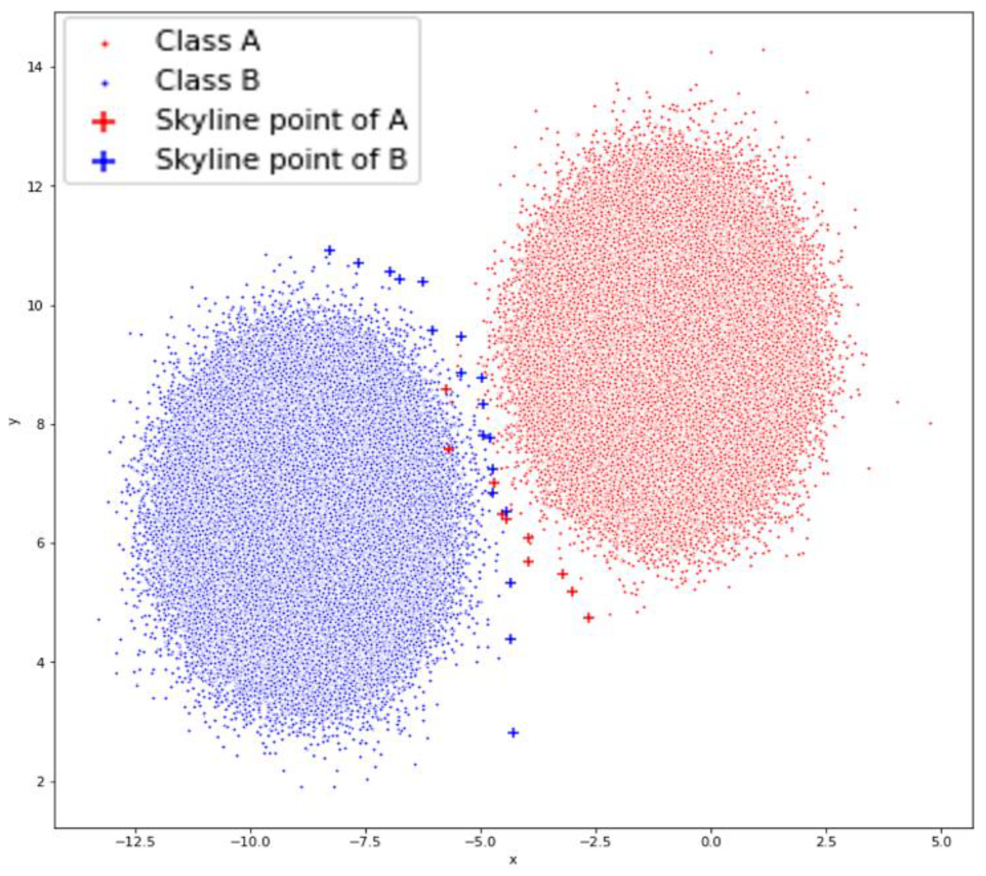
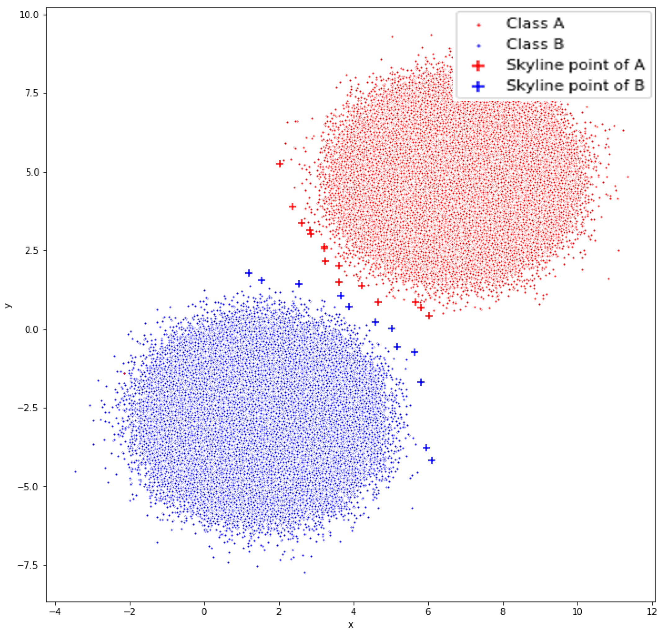
The synthetic dataset (Figure 9) was constructed to have a large number of points in order to present how the method behaves in classifying a large dataset. The first of the synthetic datasets (Figure 9) is the one that stresses our method the most since the two classes slightly overlap.

As presented in

Table 6. Single skyline on the synthetic Dataset I.

Method	k
	1	2	3	4	5	6
SKY–NN (%)	73.24	85.77	89.76	86.71	84.83	83.17
Parzen (%)	94.66	99.70	99.91	99.98	99.99	99.99

,

Table 7. Double skyline on the synthetic Dataset I.

Method	k
	1	2	3	4	5	6
SKY–NN (%)	91.01	93.87	93.87	93.78	93.48	93.23
Parzen (%)	99.06	99.68	99.83	99.86	99.89	99.91

,

Table 8. Opposite skyline on the synthetic Dataset I.

Method	k
	1	2	3	4	5	6
SKY–NN (%)	99.99	99.99	99.99	99.99	99.99	99.99
Parzen (%)	99.94	99.96	99.98	99.99	99.99	99.99

and

Table 9. Smart skyline on the synthetic Dataset I.

Method	k
	1	2	3	4	5	6
SKY–NN (%)	99.98	99.98	99.98	99.98	99.97	99.96
Parzen (%)	99.97	99.99	99.99	100	99.99	100

, the Parzen approach outperforms the SKY–NN approach. This reveals that in this slightly overlapping scenario the distance metric that is used in the SKY–NN approach does not always infer the correct prediction in comparison to the probabilistic nature of the Parzen approach. As far as the skyline identification method the single (Table 6) and double (Table 7) skyline approaches perform worse than the opposite (Table 8) and smart (Table 9) skyline, especially when the number k of selected points is small.

The polynomial curve-fitting approach (

Table 10. Polynomial curve-fitting on the synthetic Dataset I.

Degree	Single Skyline	Double Skyline	Opposite Skyline	Smart Skyline
2nd	95.42	99.87	94.44	82.50
3rd	98.57	60.60	99.82	98.39
5th	99.92	99.86	99.72	97.99
7th	99.92	99.33	99.81	93.49
8th	99.95	99.86	99.91	99.90
11th	99.99	99.97	99.93	99.92

) shows that even with a small degree polynomial curves the method performs well, and its accuracy increases as the polynomial degree increases since it better describes the overlapping regions. From all the skyline approaches, the single skyline performs best, since the selected skyline points best describe the boundaries.

Table 11. SKY–SVM on the synthetic Dataset I.

Method	Single Skyline	Double Skyline	Smart Skyline
Accuracy	99.99	99.92	97.65
Time	7270	8068	8182

shows that the SKY–SVM approach is very accurate and performs better than the polynomial curve-fitting approach. Despite that the SKY–SVM is slower that the SKY–NN and Parzen approach.

5.2. Synthetic Dataset II

The second synthetic dataset (Figure 10) is an easier case than the previous one for our method, since the classes are very close, but not overlapping. In the single skyline

Table 12. Single skyline on the synthetic Dataset II.

Method	k
	1	2	3	4	5	6
SKY–NN (%)	99.98	99.96	99.87	99.82	99.75	99.69
Parzen (%)	100	100	100	100	100	100

) the probabilistic approaches perform better. The double skyline (

Table 13. Double skyline on the synthetic Dataset II.

Method	k
	1	2	3	4	5	6
SKY–NN (%)	100	100	99.99	99.99	99.98	99.97
Parzen (%)	100	100	100	100	100	100

), which defines the boundaries better by using more points, works considerably better than all the methods, while the methods on

Table 14. Opposite skyline on the synthetic Dataset II.

Method	k
	1	2	3	4	5	6
SKY–NN (%)	100	100	100	100	100	100
Parzen (%)	100	100	100	100	100	100

and

Table 15. Smart skyline on the synthetic Dataset II.

Method	k
	1	2	3	4	5	6
SKY–NN (%)	100	100	100	100	100	100
Parzen (%)	100	100	100	100	100	100

perform very well even with a small k value.

This time, for the polynomial curve-fitting approach (

Table 16. Polynomial curve-fitting on the synthetic Dataset II.

Degree	Single Skyline	Double Skyline	Opposite Skyline	Smart Skyline
2nd	100.00	100.00	99.94	100.00
3rd	33.62	100.00	99.44	72.88

), we present the cases where the minimum polynomial degree can achieve the best results. In this case, even a 2nd degree polynomial achieves 100% accuracy.

Table 17. SKY–SVM on the synthetic Dataset II.

Method	Single Skyline	Double Skyline	Smart Skyline
Accuracy (%)	100	100	99.90
Time (ms)	7719	8779	7864

presents the accuracy and the time needed by the SKY–SVM method to perform a classification task. The method performs better than in the Dataset I with slightly better time.

5.3. Synthetic Dataset III

The third and last synthetic dataset (Figure 11) is the easiest case for our method, since the classes have a degree of clearance between them in such a way that a straight line could easily distinguish them. In this case all the approaches (

Table 18. Single skyline on the synthetic Dataset III.

Method	k
	1	2	3	4	5	6
SKY–NN (%)	99.95	99.91	99.96	99.97	99.98	99.97
Parzen (%)	99.68	99.79	99.86	99.93	99.97	99.98

,

Table 19. Double skyline on the synthetic Dataset III.

Method	k
	1	2	3	4	5	6
SKY–NN (%)	99.99	99.98	99.99	99.99	99.99	99.99
Parzen (%)	99.84	99.85	99.86	99.86	99.86	99.88

,

Table 20. Opposite skyline on the synthetic Dataset III.

Method	k
	1	2	3	4	5	6
SKY–NN (%)	100	100	100	100	100	100
Parzen (%)	100	100	100	100	100	100

and

Table 21. Smart skyline on the synthetic Dataset III.

Method	k
	1	2	3	4	5	6
SKY–NN	100	100	100	100	100	100
Parzen	100	100	100	100	100	100

) and especially the one of Table 18 and Table 19 perform very well.

Again—as with the previous approaches—the polynomial curve-fitting approach (

Table 22. Polynomial curve-fitting on the synthetic Dataset III.

Degree	Single Skyline	Double Skyline	Opposite Skyline	Smart Skyline
2nd	100	100	100	100

), performs very well for a 3rd degree polynomial.

Table 23. SKY–SVM on the synthetic Dataset III.

Method	Single Skyline	Double Skyline	Smart Skyline
Accuracy (%)	100	100	99.97
Time (ms)	7763	10,019	10,229

reveals that the SKY–SVN with the single skyline is the fastest and more accurate between the double and smart skyline.

5.4. Real Dataset

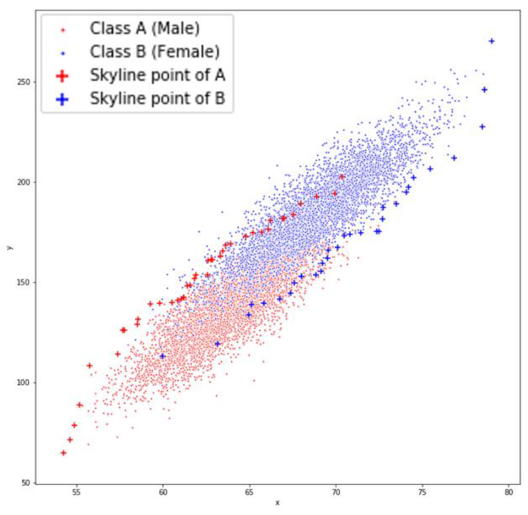
The real dataset (Figure 12) is the one that stresses our method the most since the classes have a high degree of overlap. Additionally, as it will be presented, the correlated nature of the classes also affects the performance of our methods. In this case the value of k skyline points that are selected for the classification task varies from 7 to 13, since it gives more accurate results.

As presented in

Table 24. Single skyline on the real dataset.

Method	k
	7	8	9	10	11	12	13
SKY–NN (%)	92.40	91.80	91.30	90.83	90.87	90.80	90.93
Parzen (%)	71.67	72.73	77.27	83.20	86.37	87.40	87.67

, in this scenario the SKY–NN approach performs better than the Parzen approach. In addition, the SKY–NN method needs less Skyline points to infer to a correct result than the Parzen method showing that the SKY–NN method is more suitable in cases where the dataset is corelated. The double (

Table 25. Double skyline on the real dataset.

Method	k
	7	8	9	10	11	12	13
SKY–NN (%)	86.66	85.96	86.1	86.4	86.3	86.3	86.1
Parzen (%)	65.66	67.2	69.13	71.8	74.36	76.76	78.56

) and opposite (

Table 26. Opposite skyline on the real dataset.

Method	k
	7	8	9	10	11	12	13
SKY–NN (%)	87.66	88.1	88	88.1	88.06	87.76	87.23
Parzen (%)	62.76	62.23	61.46	60.66	61.06	61.8	64.56

) skyline perform worse than the single and the performance of the Parzen approach degrades significantly. This is due to the large number of skyline points produced that do not always infer the correct result. The SKY–NN method with the smart (

Table 27. Smart skyline on the real dataset.

Method	k
	7	8	9	10	11	12	13
SKY–NN (%)	89.46	89.23	89.06	88.76	89	89.03	89.06
Parzen (%)	76.32	77.23	82.247	88.4	91.32	92.5	92.78

) skyline has slightly better results than the double and opposite skyline even with a smaller number of skyline points meaning that the smart skyline defines the boundaries better with fewer points in this case. Overall, the single and smart skyline have comparable results on this dataset.

The polynomial curve-fitting approach (

Table 28. Polynomial curve-fitting on the real dataset.

Degree	Single Skyline	Double Skyline	Opposite Skyline	Smart Skyline
2nd	87	72	69	86
3rd	82.04	68	65	81.5

) shows that in this case a small degree polynomial gives better results in comparison to the case of the synthetic dataset.

The accuracy of the SKY–SVM approach for the real dataset is presented in

Table 29. SKY–SVM on the real dataset.

Method	Single Skyline	Double Skyline	Smart Skyline
Accuracy (%)	90.06	85.3	90.03
Time (ms)	87.5	100.5	99.8

. As with the synthetic dataset the SKY–SVM approach is very accurate but takes more time to infer to a result than the SKY–NN and Parzen approach. In this case the single and smart skyline have similar results.

With the use of the three synthetic datasets we present that the factor of distance between the classes does not affect the final result as opposed to the overlapping factor of classes. Based on Dataset II and III, which are not overlapping and have a variable distance between the classes, we see that all the proposed approaches can always infer to a correct result. In the case of the Dataset I for which the classes slightly overlap, we can see that the methods which are affected the most are the single and double skyline which need a larger number of k to infer to a correct result, while the opposite and smart can still infer the correct result even with a small number of k. The use of larger k-value due to the overlapping nature of classes is also presented in the case of the real dataset.

Overall, the SKY–NN approach is faster than the Parzen approach, while the number of k selected skyline points affects both methods. In addition, the SKY–NN performs better in small datasets while the Parzen in the bigger ones. In a correlated dataset, the SKY–NN performs better with fewer skyline points while the Parzen approach performs better in non-correlated datasets. The Polynomial approach works best when the polynomial function can describe the boundaries of the dataset and, in general, it is slower than the SKY–NN and Parzen method. The correlation of the dataset affects the degree of the polynomial function. The SKY–SVM approach is the slowest method and is not affected by the correlation but achieves very good results. In cases where the classes of the dataset have a high degree of overlap, we need to use more skyline points to infer in a correct result. The single skyline approach almost in all cases achieves very good results with the least cost. The double and opposite skyline in many cases achieve very good results, but the cost is double. The smart skyline is a good alternative to the single skyline which, with small number of additional skyline points, can achieve better results.

6. Future Work

Our approach could be expanded by defining a metric of uncertainty in the classification process. Based on this metric the proposed method could automatically classify points and simultaneously compute a factor of uncertainty in every decision. If the uncertainty for classifying a given point drops to a certain threshold, human assistance could be requested. The user could easily identify the class and allow the system to refine the decision boundaries instantly and on the fly.

7. Conclusions

To the best of author’s knowledge, this is the first work that studies the use of skyline queries in a classification process. Through our experimentation we showed that the proposed method is faster than the k-NN and the SVM, but slower than the naïve Bayes, yet having comparable accuracy when classifying large datasets. The full potential of our proposed method is visible on big datasets in which the decision boundaries are better described, and the number of points selected by the skyline operator, in comparison to the whole dataset, is small. Due to the small number of points used to describe the decision boundaries, our approach needs to perform only a small number of comparisons in order to infer the correct class. This makes our approach fast and capable of handling very large datasets for which the performance of other classifiers degrades. This was presented with the case of the K-NN approach, which did not succeed to infer in a result at a reasonable time for the case of 1 M synthetic datasets. With the use of different skyline identification methods, we showed that with a broader set of skyline points we can achieve, in some cases, better results, but with additional computation cost. Our approach can also parallelize the decision boundary computation since we can compute independently and in parallel the skyline for each class which can be beneficial when using big data technologies like Hadoop. In addition, the decision boundaries can be easily updated and optimized due to the small number of points that consists them. Moreover, due to the properties and variants of the skyline, the number of points will remain small despite the increase of the dataset size or the dimensionality. Finally, the decision boundaries can be easily visualized and interpreted by a human being allowing him to fully understand the reason for which our approach inferred to a specific result in each case.

With this work, we show that skyline queries can efficiently reveal the decision boundaries between two classes and thus, could assist towards building decision support or recommendation systems. The inherited properties of Pareto principal make them a good candidate in a big data environment.