Generalized Multiscale Finite Element Method for Elastic Wave Propagation in the Frequency Domain

Abstract

In this work, we consider elastic wave propagation in fractured media. The mathematical model is described by the Helmholtz problem related to wave propagation with specific interface conditions (Linear Slip Model, LSM) on the fracture in the frequency domain. For the numerical solution, we construct a fine grid that resolves all fracture interfaces on the grid level and construct approximation using a finite element method. We use a discontinuous Galerkin method for the approximation by space that helps to weakly impose interface conditions on fractures. Such approximation leads to a large system of equations and is computationally expensive. In this work, we construct a coarse grid approximation for an effective solution using the Generalized Multiscale Finite Element Method (GMsFEM). We construct and compare two types of the multiscale methods—Continuous Galerkin Generalized Multiscale Finite Element Method (CG-GMsFEM) and Discontinuous Galerkin Generalized Multiscale Finite Element Method (DG-GMsFEM). Multiscale basis functions are constructed by solving local spectral problems in each local domains to extract dominant modes of the local solution. In CG-GMsFEM, we construct continuous multiscale basis functions that are defined in the local domains associated with the coarse grid node and contain four coarse grid cells for the structured quadratic coarse grid. The multiscale basis functions in DG-GMsFEM are discontinuous and defined in each coarse grid cell. The results of the numerical solution for the two-dimensional Helmholtz equation are presented for CG-GMsFEM and DG-GMsFEM for different numbers of multiscale basis functions.

1. Introduction

Understanding the complex processes in fractured media is necessary in many real world applications, for example, in exploring and developing hydrocarbon reservoirs. Fractured media are characterized by a complex fracture distribution and presence of the fractures at multiple scales [1,2]. Moreover, fractures are characterized as thin and long interfaces. Numerical methods for the solution of the problems in fractured media are being actively developed in recent years. In Reference [3] the authors developed finite difference schemes for modeling wave propagation in a fractured medium. Fractured media are derived when the fracture interfaces are aligned with the boundaries of the finite-difference grid. For flow problems in fractured media, the multiscale finite volume method on unstructured grids for discrete fracture model (MS-DFM) is presented in Reference [4]. The use of unstructured grids requires rather complicated grid generators and significantly increases the run time, also, its use is undesirable when the number of fractures is large. In Reference [5] the author proposed an approach called Chimera Grid Approach. This technique avoids the use of curvilinear or unstructured grids, replacing them with a set of arbitrary rotated rectangular grids. In Reference [6], the authors proposed an approach to modeling the propagation of seismic waves in a medium containing subvertical fractured inhomogeneities using the grid-characteristic method on structural grids without constructing additional grids. To simulate wave propagation in fractured media, the discontinuous Galerkin (DG) method is widely used. The main disadvantage of the DG method is the excessive use of memory due to a large number of degrees of freedom. But in Reference [7] the authors propose an Enriched Galerkin finite element method (EGM) for elastic wave propagation. EGM formulated by enriching the conforming continuous Galerkin finite element method with piecewise constant functions.

In this work, we consider elastic wave propagation in fractured media. The Linear Slip Model (LSM) is used to simulate the influence of the fracture on the distribution of the seismic field, where the stress components are proportional to the displacement [1,2]. LSM requires constructing a fine grid that resolves all fracture interfaces on the grid level, which leads to a very large system of equations. To construct a suitable mathematical model for seismic wave propagation, multiscale methods or homogenization techniques are used. Homogenization or effective media theories replace a heterogeneous rock with an equivalent homogeneous rock, where the corresponding properties are calculated under the static-deformation regimes. An overview and comparison of the existing effective media theories for fractured formations is presented in Reference [8]. The authors consider a three-dimensional formulation and use direct finite-element simulations in order to calculate the effective properties of the fractured media. Direct computational studies provide an independent verification of theoretical predictions and can be used to examine realistic fracture models that violate the conventional assumptions, where fractures have notoriously irregular shape and can form interconnected networks. On the other hand, this approach is computationally expensive for complex fracture distributions. Moreover, the errors of the homogenization methods depend on the coarse-grid mesh.

In the multiscale methods, a central research problem is constructing the coarse grid approximation for faster results, where multiscale basis functions are computed on a fine grid to capture the influence of fractures and other heterogeneity [9,10,11,12,13,14]. We consider seismic waves in fractured media and construct multiscale basis functions for coarse grid simulations in the two-dimensional formulation [15,16,17,18,19]. These multiscale basis functions can capture the influence of the fractures on a coarse grid and reduce the number of unknowns in calculations. Multiscale basis functions are constructed using the solution of the local spectral problem on a fine grid in each coarse grid cell. In our previous work, we presented GMsFEM for elastic wave propagation in time domain in fractured media [15,20].

In this paper, we construct two types of multiscale spaces to solve the Helmholtz equation for fractured media. The numerical implementation is based on the global projection approach to construct a coarse-grid approximation. The local spectral problems that we used for selecting the dominant modes are frequency-independent. The presented method has much in common with classical homogenization methods and, therefore, the applicability is limited by low frequencies. We present numerical results and consider several test cases with different fracture configurations. Numerical simulations show that the method is accurate for complex cases and can significantly reduce the dimension of the system.

The work is organized as follows—in Section 2, we provide the mathematical model of the Helmholtz problem in fractured media and construct a fine grid approximation using the finite element method in Section 3. In Section 4, we present a coarse grid approximation using the Generalized Multiscale Finite Element Method (GMsFEM) algorithm, where we describe constructing of the two types of multiscale basis functions—(1) Continuous Galerkin Generalized Multiscale Finite Element Method (CG-GMsFEM) with continuous multiscale basis functions and (2) Discontinuous Galerkin Generalized Multiscale Finite Element Method (DG-GMsFEM) with discontinuous multiscale basis functions. Finally, numerical results are presented in Section 5.

2. Problem Formulation

We consider a problem in a fractured medium. Let $\mathsf{\Omega }\subset R^d$ is the bounded computational domain and $\gamma \subset R^{d-1}$ is the fracture interface, $d=2$ (see Figure 1 for illustration). The elastic wave propagation is described by Helmholtz equation in the computational domain $\mathsf{\Omega }$ [21,22]

$$-\mathrm{div}\sigma \left(u\right)-{\omega }^2\rho u=f,x\in \mathsf{\Omega },$$

(1)

where $\omega$ is the frequency, $\sigma$ is the stress tensor, $\rho$ is the density and f is the source function.

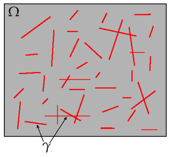
Figure 1. Illustration of the computational domain $\mathsf{\Omega }$ (grey color) and fractures $\gamma$ (red color).

We have linear elastic stress-strain constitutive relation

$$\sigma \left(u\right)=2\mu \epsilon \left(u\right)+\lambda \mathrm{div}u\mathcal{I},\epsilon \left(u\right)=\frac{1}{2}(\mathrm{grad}u+{\left(\mathrm{grad}u\right)}^T),$$

(2)

where $\mathcal{I}$ is the unit tensor, $\lambda$ and $\mu$ are the Lame parameters.

In this paper, we focus on the two-dimentional formulation of the problem. Since the problem is considered in fractured media, for numerical simulations of the elastic wave equation, the linear-slip model (LSM) is applied on the fracture interface $\gamma$ [23,24]. Namely, we assume the fractures have a vanishing width across which the traction is considered continuous. Following the linear-slip model, we have a linear relation between the traction vector and the magnitude of the discontinuity in the displacement field as follows

$$\left[u\right]=Z\sigma n,x\in \gamma ,$$

(3)

where $\left[u\right]$ is the jump of the displacement field at the fracture, $\sigma n$ is the traction vector at the surface of the fracture $\gamma$ and Z is the fracture compliance matrix. In the two-dimensional isotropic case, the compliance matrix is diagonal and positive definite

$$Z=\left[\begin{array}{cc}{z}_1& 0\\ 0& z_2\end{array}\right],$$

where $z_1$ and $z_2$ are the normal and tangential compliance. In the numerical simulations we will use a scalar fracture compliance, with $z=z_1=z_2$ and $Z=z\mathcal{I}$, where $\mathcal{I}$ is the identity matrix [23,24].

In the computations we use the first order absorbing boundary condition, because the energy of waves needs to be absorbed in artificial boundaries in order to avoid spurious reflections caused by the finite computational domain [25]

$$i\rho \omega Au=-\sigma n,x\in \partial \mathsf{\Omega },$$

(4)

where

$$A=\left[\begin{array}{cc}{n}_1& n_2\\ -n_2& n_1\end{array}\right]\left[\begin{array}{cc}{c}_p& 0\\ 0& c_s\end{array}\right]\left[\begin{array}{cc}{n}_1& -n_2\\ n_2& n_1\end{array}\right].$$

Here $n=(n_1,n_2)$ is the outward normal to the boundary and $c_p=\sqrt{(\lambda +2\mu )/\rho },c_s=\sqrt{\mu /\rho }$ are the S- and P-wave velocities. We will impose this absorbing condition in the variational formulation of the problem.

3. Fine Grid Approximation

We use the Interior Penalty Discontinuous Galerkin (IPDG) finite element method for the fine-grid approximation. IPDG method allows for discontinuities in the displacement field to simulate fractures with the linear-slip model [26,27,28]. We construct a fine grid for fracture domain $\mathsf{\Omega }$ that resolve fracture interface $\gamma$ on the grid level.

Let ${\mathcal{T}}_h$ be a triangulation of the computational domain $\mathsf{\Omega }$ and h be the fine mesh size. We define ${\mathsf{\Gamma }}_h$ as the set of all the interior faces between the elements ${\mathcal{T}}_h$, ${\mathsf{\Gamma }}_c\subset {\mathsf{\Gamma }}_h$ be the subset of all faces, where the displacement field is continuous and ${\mathsf{\Gamma }}_{\gamma }\subset {\mathsf{\Gamma }}_h$ be the subset of facet that represent fractures, ${\mathsf{\Gamma }}_b$ is a subset of faces on the boundary and ${\mathsf{\Gamma }}_h={\mathsf{\Gamma }}_c\cup {\mathsf{\Gamma }}_{\gamma }\cup {\mathsf{\Gamma }}_b$. Let $e\in {\mathsf{\Gamma }}_h$ be the edge between the elements ${\iota }_1$ and ${\iota }_2$, then the average $\{·\}$ and jump $\left[·\right]$ of a vector function u on e are given by

$$\left\{u\right\}=\left({u\mid }_{{\iota }_1}+{u\mid }_{{\iota }_2}\right)/2,\left[u\right]={u\mid }_{{\iota }_1}-{u\mid }_{{\iota }_2}.$$

The variational formulation of the elastic wave equation using the interior penalty discontinuous Galerkin method in fractured media is defined as follows: find $u\in V$ such that

$$\begin{array}{cc}\hfill & \sum _{\iota \in {\mathcal{T}}_h}{\int }_{\iota }(\sigma \left(u\right),\epsilon \left(\overline{v}\right))dx-\sum _{\iota \in {\mathcal{T}}_h}{\int }_{\iota }\rho {\omega }^{2}u\overline{v}dx+i\sum _{e\in {\mathsf{\Gamma }}_b}{\int }_e\rho \omega Au\overline{v}ds\hfill \\ \hfill & -\sum _{e\in {\mathsf{\Gamma }}_c}{\int }_e\left\{\tau \left(u\right)\right\}\left[\overline{v}\right]ds-\sum _{e\in {\mathsf{\Gamma }}_c}{\int }_e\left\{\tau \left(\overline{v}\right)\right\}\left[u\right]ds+\sum _{e\in {\mathsf{\Gamma }}_c}\frac{\zeta }{h_{\iota }}{\int }_e\{\lambda +2\mu \}\left[u\right]\left[\overline{v}\right]ds\hfill \\ \hfill & +\sum _{e\in {\mathsf{\Gamma }}_f}{\int }_e{Z}^{-1}\left[u\right]\left[\overline{v}\right]ds=\sum _{\iota \in {\mathcal{T}}_h}{\int }_{\iota }f\overline{v}dx,\hfill \end{array}$$

(5)

where $\zeta$ is the penalty parameter, $\tau \left(u\right)=\sigma n$ is the traction vector, V is a suitable finite dimension function space. Here u is the complex valued function and $u={\sum }_j{u}_j{\varphi }_j$, ${\varphi }_j$ are linear basis functions for the fine scale approximation.

By definition of the following bilinear and linear forms

$$m(u,v)=\sum _{\iota \in {\mathcal{T}}_h}{\int }_{\iota }\rho u\overline{v}dx,b(u,v)=\sum _{e\in {\mathsf{\Gamma }}_b}{\int }_e\rho Au\overline{v}ds,l\left(v\right)=\sum _{\iota \in {\mathcal{T}}_h}{\int }_{\iota }f\overline{v}dx,$$

(6)

$$\begin{array}{cc}\hfill a_{DG}(u,v)& =\sum _{\iota \in {\mathcal{T}}_h}{\int }_{\iota }(\sigma \left(u\right),\epsilon \left(\overline{v}\right))dx+\sum _{e\in {\mathsf{\Gamma }}_f}{\int }_e{Z}^{-1}\left[u\right]\left[\overline{v}\right]ds\hfill \\ \hfill & -\sum _{e\in {\mathsf{\Gamma }}_c}{\int }_e\left\{\tau \left(u\right)\right\}\left[\overline{v}\right]ds-\sum _{e\in {\mathsf{\Gamma }}_c}{\int }_e\left\{\tau \left(\overline{v}\right)\right\}\left[u\right]ds+\sum _{e\in {\mathsf{\Gamma }}_c}\frac{\zeta }{h_{\iota }}{\int }_e\{\lambda +2\mu \}\left[u\right]\left[\overline{v}\right]ds,\hfill \end{array}$$

(7)

we obtain the following formulation

$$a_{DG}(u,v)-{\omega }^{2}m(u,v)+i\omega b(u,v)=l\left(v\right).$$

(8)

We can write the complex valued problem in matrix form

$$(K_h-{\omega }^2{M}_h+i\omega B_h)U=F_h,$$

(9)

where $K_h$ is the stiffness matrix, $M_h$ is the mass matrix and $B_h$ is the boundary mass matrix.

4. Multiscale Method on the Coarse Grid

In this section, we describe construction of the multiscale basis functions and coarse grid approximation [10,15,17,29,30,31]. For construction of the coarse grid approximation, we will use a projection approach and define a projection matrix R. We consider two types of the multiscale basis functions: (1) CG-GMsFEM with continuous multiscale basis functions and (2) DG-GMsFEM with discontinuous multiscale basis functions in coarse cells. By the algorithmic point of view, the differences between two considered methods are concentrated on the definition of the local domains and construction of the multiscale basis functions. After construction, we collect multiscale basis functions into the projection matrix R. Therefore, we will define construction of the two projection matrices $R_{CG}$ and $R_{DG}$.

The main steps of the multiscale method is similar for both approaches (CG-GMsFEM and DG-GMsFEM). We have following steps in the multiscale computational algorithm:

1.

construction of the coarse grid and local domains;

2.

construction of the multiscale basis functions by the solution of the local eigenvalue problem in each local domains;

3.

construction of the projection matrix R (from fine grid to coarse grid) using computed multiscale basis functions;

4.

construction of the fine grid system and projection to the coarse grid using matrix R;

5.

solution of the reduced order model and reconstruction of the fine grid solution.

We start with definition of the coarse grid. Let ${\mathcal{T}}_H$ be the coarse grid partitioning of the domain $\mathsf{\Omega }$, ${\mathcal{T}}_H={\cup }_{i=1}^{N_c}{K}_i$ with mesh sizes $H\gg h>0$, where $K_i$ is the coarse cell and $N_c$ is number of coarse cells. We note that, the coarse grid edges are conforming with the fine grid. In this work, we use a structured coarse grid with quadrilateral coarse cells. In general, shape of the coarse grid can be complex (unstructured coarse grid) and can be constructed, for example, using traditional mesh partitioning.

Next, we define local domains. We have

• for CG-GMsFEM, the local domain ${\omega }_i$ are defined as a coarse neighborhood that contains four coarse grid quadrilateral cells around coarse grid node, where $i=1,\dots ,N_v$ and $N_v$ is the number of the coarse grid nodes (see Figure 2 for illustration);
  

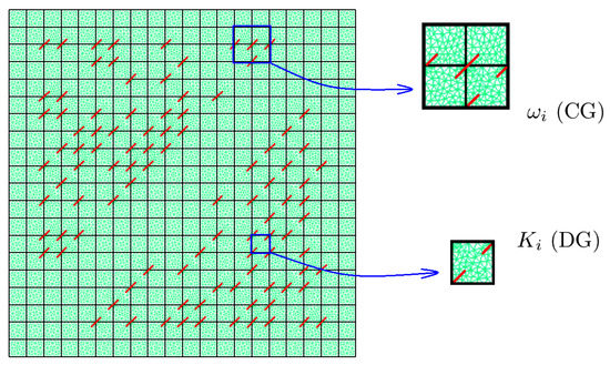  Figure 2. Coarse grid and local domains illustration for CG-GMsFEM and DG-GMsFEM. Fractures are depicted in red color. Structured $20\times 20$ coarse grid (black color). Unstructured fine grid (green color) with triangular elements that conformed with fractures.
• for DG-GMsFEM, the local domain is the coarse grid cell $K_i$, where $i=1,\dots ,N_c$ and $N_c$ is the number of the coarse grid cells.

After that, we solve local eigenvalue problems in each local domains in order to construct the multiscale basis functions and using them we define a projection matrices $R_{CG}$ and $R_{DG}$. The form of the eigenvalue problems will be presented later for CG-GMsFEM and DG-GMsFEM.

Finally, the multiscale reduced order discrete system can be calculated by projecting the fine-scale matrices onto the coarse grid with the global projection matrix $R=R_{CG}$ or $R=R_{DG}$

$$(K_H-{\omega }^2{M}_H+i\omega B_H)U_H=F_H,$$

(10)

where $U_H$ is the complex valued solution on multiscale space, $M_H$ and $K_H$ are the coarse-scale mass and stiffness matrices, and $B_H$ is the coarse-scale boundary mass matrix

$$M_H=R{M}_h{R}^T,K_H=R{K}_h{R}^T,B_H=R{B}_h{R}^T,F_H=R{F}_h.$$

(11)

After calculation of the coarse-scale solution $U_H$, we can recover the fine-scale solution by $U_{ms}=R^T{U}_H$.

Next, we consider construction of multiscale basis functions based on two approaches—continuous Galerkin method and discontinuous Galerkin method.

4.1. Multiscale Basis Functions for CG-GMsFEM

In CG-GMsFEM, the local domain ${\omega }_i$ is obtained by the combining all the coarse cells around one vertex of the coarse grid. To construct the multiscale basis functions, we start with the solution of the following local eigenvalue problem in ${\omega }_i$

$$a_{CG}({\varphi }^{{\omega }_i},v)=\eta s({\varphi }^{{\omega }_i},v),\forall v\in V_h\left({\omega }_i\right),$$

(12)

where

$$s({\varphi }^{{\omega }_i},v)={\int }_{{\omega }_i}\rho {\varphi }^{{\omega }_i}vds.$$

For definition of the multiscale basis functions, we select the first M eigenvectors ${\varphi }_1^{{\omega }_i}$, ${\varphi }_2^{{\omega }_i}$, …, ${\varphi }_M^{{\omega }_i}$ corresponding to the first M smallest eigenvalues ${\eta }_1\le {\eta }_2\le \dots \le {\eta }_M$. In order to construct continuous multiscale space, we multiply eigenvectors to the partition of unity functions ${\chi }_i$ in local domain ${\omega }_i$ and define local projection matrices $R_{CG,i}$ ($i=1,\dots ,N_v$) as follows

$$R_{CG,i}={\left[{\psi }_1^{{\omega }_i},{\psi }_2^{{\omega }_i},\dots ,{\psi }_M^{{\omega }_i}\right]}^T,$$

(13)

where ${\psi }_j^{{\omega }_i}={\chi }_i{\varphi }_j^{{\omega }_i}$ ($j=1,\dots ,M$) and ${\chi }_i$ is the piece-wise bi-linear shape function on the coarse grid that equals to 1 at the coarse vertex $x_i$, equals to 0 at all other coarse vertices.

The global projection matrix defined as follows

$$R_{CG}=(R_{CG,1},R_{CG,2},\dots ,R_{CG,N_v}).$$

(14)

4.2. Multiscale Basis Functions for DG-GMsFEM

In contrast to the continuous Galerkin method, the discontinuous Galerkin approach treats local domain as a coarse cells $K_i$. For DG-GMsFEM, we construct two local multiscale spaces (boundary and interior) by solution of the local eigenvalue problems on each coarse grid cell $K_i\in {\mathcal{T}}_H$. Boundary and interior basis functions are both defined in the local domain $K_i$ up to fine grid resolution, ${\varphi }_j^{K_i,\alpha }\in V_h\left(K_i\right)$, $j=1,\dots M_{\alpha }$, $\alpha =b,o$ (indices b and o refer to the boundary and internal basis, respectively). Multiscale basis functions differ by the definition of the local spectral problem.

To construct the boundary multiscale basis functions, we solve following spectral problem in $K_i$:

$$a_{DG}({\varphi }^{K_i,b},v)={\eta }^b{s}^b({\varphi }^{K_i,b},v),\forall v\in V_h\left(K_i\right),$$

(15)

where

$$s^b({\varphi }^{K_i,b},v)={\int }_{\partial K_i}\rho {\varphi }^{K_i,b}vds.$$

To construct a boundary multiscale basis functions, we select the first $M_b$ eigenvectors ${\varphi }_1^{K_i,b}$, ${\varphi }_2^{K_i,b}$, …, ${\varphi }_{M_b}^{K_i,b}$ corresponding to the first $M_b$ smallest eigenvalues ${\eta }_1^b\le {\eta }_2^b\le \dots \le {\eta }_{M_b}^b$, and define following local projection matrix

$$R_{DG,i}^b={\left[{\varphi }_1^{K_i,b},{\varphi }_2^{K_i,b},\dots ,{\varphi }_{M_b}^{K_i,b}\right]}^T.$$

(16)

The interior multiscale basis functions are defined to capture interior eigenmodes for $K_i$ and use following spectral problem to identify the important modes

$$\begin{array}{c}{a}_{DG}({\varphi }^{K_i,o},v)={\eta }^o{s}^o({\varphi }^{K_i,o},v),\end{array}$$

(17)

where

$$s^o({\varphi }^{K_i,o},v)={\int }_{K_i}\rho {\varphi }^{K_i,o}vds,$$

with homogeneous Dirichlet boundary conditions.

We select the first $M_o$ eigenvectors ${\varphi }_1^{K_i,o},{\varphi }_2^{K_i,o},\dots ,{\varphi }_{M_o}^{K_i,o}$ corresponding to the first $M_o$ smallest eigenvalues ${\eta }_1^o\le {\eta }_2^o\le \dots \le {\eta }_{M_o}^o$. We define following local matrix

$$R_{DG,i}^o={\left[{\varphi }_1^{K_i,o},{\varphi }_2^{K_i,o},\dots ,{\varphi }_{M_o}^{K_i,o}\right]}^T.$$

(18)

The global projection matrix defined as follows

$$R_{DG}=(R_{DG,1}^b,R_{DG,1}^o,R_{DG,2}^b,R_{DG,2}^o,\dots ,R_{DG,N_v}^b,R_{DG,N_v}^o).$$

(19)

The complete stability and convergence analysis of the GMsFEM was presented in References [17,30]. We expect a similar behavior to the presented algorithms. The error of both multiscale methods depends on the coarse-scale mesh size (H) and the number of multiscale basis functions ($\mathsf{\Lambda }=1/{\lambda }_{M+1}$) (see Theorem 1 and 3 in Reference [17]).

5. Numerical Results

In this section, we present the numerical results for the coarse-scale approximation using multiscale basis functions. We consider Continuous Galerkin (CG) and Discontinuous Galerkin (DG) methods in GMsFEM. The basis functions of the multiscale space are constructed following the procedure described above.

For numerical simulations, we use the following parameters. Computational domain is presented in Figure 3 and have dimensions $\mathsf{\Omega }=[0,L_x]\times [0,L_y]$ with $L_x=L_y=500$ [m]. In Figure 4, we show a fine grid (green color) and coarse grid (blue color) for two test geometries with different length of fractures:

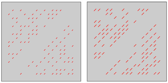
Figure 3. Geometry 1 and 2 with 100 straight fractures. Fractures $\gamma$ are depicted in red color. Domain $\mathsf{\Omega }={[0,L]}^2$ is depicted in gray color with $L=500$ m. Left: Geometry 1 with fractures length 10 m and ${45}^{\circ }$ orientation angle. Right: Geometry 2 with fractures length 20 m and ${45}^{\circ }$ orientation angle.

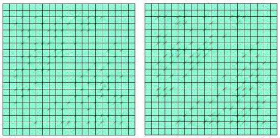
Figure 4. Computational grids for Geometry 1 and 2 with 100 straight fractures. Fractures are depicted in red color. Structured coarse grid (black color) with 400 square cells. Unstructured fine grid (green color) with triangular elements that conformed with fractures. Left: Geometry 1 with fractures length 10 m and ${45}^{\circ }$ orientation angle.The fine grid contains 31,752 triangle elements. Right: Geometry 2 with fractures length 20 m and ${45}^{\circ }$ orientation angle. The fine grid contains 32,616 triangle elements.

• Geometry 1: Fine grid contains 16,077 vertices and 31,752 triangle elements.
• Geometry 2: Fine grid contains 16,509 vertices and 32,616 triangle elements.

Note that, the fine grids are unstructured grids that resolve the fractures. Coarse grid is uniform and contains 441 vertices and 400 rectangular elements.

We set the source term $f\left(x\right)=G\left(x\right)P\left(\theta \right)$, where $P\left(\theta \right)=(cos\theta ,sin\theta )$ is the polar angle of the source force vector with $\theta =0$ and the spatial function $G\left(x\right)$ is defined as point source, $G\left(x\right)=\delta (x-x_0)$ with $x_0=(250,250)$ assigned as the center of the computational domain. We take penalty parameters $\zeta =4$ and run simulations for $\omega =2\pi f_0$ with $f_0=5,10,15$. For numerical simulation, we set following parameters $\mu =28.571\times {10}^9$ [Pa], $\lambda =23.077\times {10}^9$ [Pa] and $\rho =2300$ [kg/m${}^3$]. For fracture compliance matrix Z in (3), we use $z_1=z_2={10}^7$ [m/Pa].

To compare a results, we calculate following relative errors in %

$$e_{L_2}=\sqrt{\frac{{\int }_{\mathsf{\Omega }}(u^{ms}-u,u^{ms}-u)dx}{{\int }_{\mathsf{\Omega }}(u,u)dx}}·100\%,$$

$$e_{H_1}=\sqrt{\frac{{\int }_{\mathsf{\Omega }}(\sigma (u^{ms}-u),\epsilon (u^{ms}-u))dx}{{\int }_{\mathsf{\Omega }}(\sigma \left(u\right),\epsilon \left(u\right))dx}}·100\%,$$

where $u^{ms}$ and u are multiscale solutions and reference solutions (fine grid solution).

In Figure 5 and Figure 6, we present real parts $Re\left(u\right)$ of solution for Geometry 1 and 2 with $f_0=15$, where multiscale solver constructed using DG-GMsFEM. Reference (fine-grid) solution is shown on the top, and multiscale is on bottom. From the figures we can see that the length of fractures affect the solution. If we take a longer crack length, then the waves are reflected more strongly. The fine grid system that used to calculate reference solution has size $DO{F}_f$ = 190,512 for Geometry 1 and $DO{F}_f$ = 195,696 for Geometry 2. Multiscale calculations are performed for $M=25$ and the size of coarse grid system is $DO{F}_c$ = 20,000 (10% from $DO{F}_f$). Note that, the degrees of freedom are defined by the number of basis functions and the number of local domains in DG-GMsFEM and CG-GMsFEM. We have $DO{F}_c=N_v·M$ for CG-GMsFEM and $DO{F}_c=N_c·(M_o+M_b)$ for DG-GMsFEM, where $N_v$ is the number of coarse grid vertices and $N_c$ is the number of coarse grid cells.

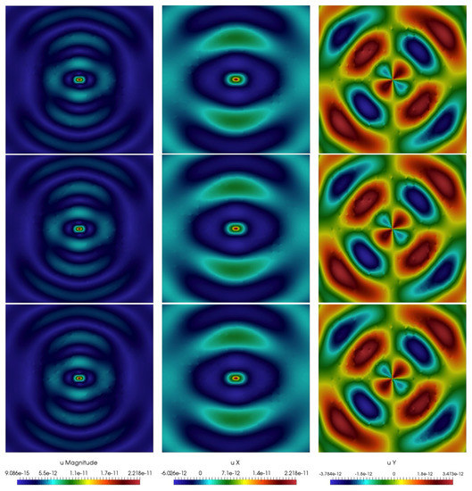
Figure 5. Numerical results for Geometry 1. Magnitude, X and Y components of displacement (from left to right). First row: reference (fine-grid) solution. Second row: multiscale solution using CG-GMsFEM. Third row: multiscale solution using DG-GMsFEM.

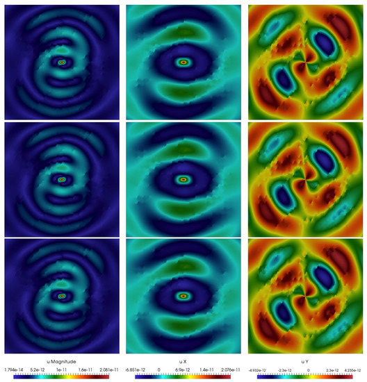
Figure 6. Numerical results for Geometry 2. Magnitude, X and Y components of displacement (from left to right). First row: reference (fine-grid) solution. Second row: multiscale solution using CG-GMsFEM. Third row: multiscale solution using DG-GMsFEM.

Relative errors are shown in Table 1 and Table 2 for two approaches proposed above and for two geometries (Figure 3). $DO{F}_c$ is number of unknowns in multiscale solver, M is the number of multiscale basis functions for CG-GMsFEM, and $M_o$ and $M_b$ are the numbers of multiscale interior and boundary basis functions for DG-GMsFEM, respectively. We observe that the larger number of multiscale basis functions can reduce errors.

Table 1. Relative errors for Continuous Galerkin Generalized Multiscale Finite Element Method (CG-GMsFEM) with different number of multiscale basis functions M. Left: Geometry 1. Right: Geometry 2.

		Geometry 1				Geometry 2
$\mathit{M}$	${\mathit{DOF}}_{\mathit{c}}$	${\mathit{e}}_{{\mathit{L}}_{\mathbf{2}}}$(%)	${\mathit{e}}_{{\mathit{H}}_{\mathbf{1}}}$(%)	$\mathit{M}$	${\mathit{DOF}}_{\mathit{c}}$	${\mathit{e}}_{{\mathit{L}}_{\mathbf{2}}}$(%)	${\mathit{e}}_{{\mathit{H}}_{\mathbf{1}}}$(%)
		$f_0=5$				$f_0=5$
5	2205	5.683	44.617	5	2205	22.032	49.143
10	4410	3.750	37.737	10	4410	3.174	37.845
15	6615	2.570	34.923	15	6615	2.944	35.137
20	8820	1.921	32.049	20	8820	3.540	32.216
25	11,025	1.591	30.422	25	11,025	3.559	30.903
50	22,050	1.187	25.187	50	22,050	2.676	25.583
		$f_0=10$				$f_0=10$
5	2205	8.717	41.269	5	2205	25.635	47.053
10	4410	5.383	34.477	10	4410	3.9745	35.073
15	6615	3.495	31.825	15	6615	3.7782	32.420
20	8820	2.567	29.241	20	8820	3.8773	29.772
25	11,025	2.184	27.861	25	11,025	3.6346	28.403
50	22,050	1.343	23.025	50	22,050	2.4719	23.345
		$f_0=15$				$f_0=15$
5	2205	19.997	42.195	5	2205	49.906	57.898
10	4410	8.927	32.913	10	4410	8.128	33.930
15	6615	5.217	30.303	15	6615	6.779	31.575
20	8820	2.970	27.818	20	8820	6.506	29.065
25	11,025	2.669	26.493	25	11,025	6.577	27.819
50	22,050	1.924	21.754	50	22,050	4.945	22.936

Table 2. Relative errors for Discontinuous Galerkin Generalized Multiscale Finite Element Method (DG-GMsFEM) with different number of multiscale basis functions $M=M_o=M_b$. Left: Geometry 1. Right: Geometry 2.

		Geometry 1				Geometry 2
$\mathit{M}$	${\mathit{DOF}}_{\mathit{c}}$	${\mathit{e}}_{{\mathit{L}}_{\mathbf{2}}}$(%)	${\mathit{e}}_{{\mathit{H}}_{\mathbf{1}}}$(%)	$\mathit{M}$	${\mathit{DOF}}_{\mathit{c}}$	${\mathit{e}}_{{\mathit{L}}_{\mathbf{2}}}$(%)	${\mathit{e}}_{{\mathit{H}}_{\mathbf{1}}}$(%)
		$f_0=5$				$f_0=5$
5	4000	86.368	99.956	5	4000	86.412	99.969
10	8000	64.157	78.074	10	8000	70.890	81.704
15	12,000	34.960	53.810	15	12,000	35.100	54.556
20	16,000	13.730	41.178	20	16,000	21.538	44.009
25	20,000	7.556	33.535	25	20,000	10.007	34.752
50	40,000	2.236	16.672	50	40,000	3.516	17.245
		$f_0=10$				$f_0=10$
5	4000	98.804	99.992	5	4000	99.136	100.004
10	8000	77.995	80.921	10	8000	87.598	86.050
15	12,000	28.137	49.248	15	12,000	31.581	50.711
20	16,000	12.443	37.775	20	16,000	19.672	40.105
25	20,000	7.534	30.598	25	20,000	9.890	31.458
50	40,000	2.069	15.541	50	40,000	3.295	16.074
		$f_0=15$				$f_0=15$
5	4000	99.264	99.986	5	4000	99.446	99.994
10	8000	92.430	86.462	10	8000	98.481	90.507
15	12,000	42.383	52.390	15	12,000	45.749	54.527
20	16,000	20.054	38.037	20	16,000	26.519	41.610
25	20,000	11.739	30.303	25	20,000	13.800	32.069
50	40,000	3.4803	15.492	50	40,000	6.327	17.354

6. Conclusions

We construct reduced order model using Generalized Multiscale Continuous Galerkin Finite Element Method (CG-GMsFEM) and Generalized Multiscale Discontinuous Galerkin Finite Element Method (DG-GMsFEM). We present numerical results for domain with fractures for two approaches to demonstrate efficiency of presented methods. Numerical results show that the presented multiscale methods give a good approximation of the solution and reduce the size of the system for both types of methods (CG- and DG-GMsFEM). We observe a good reduction of the $L_2$ errors for both methods when the number of the multiscale basis functions increases. In order to further error reduction, we will add an online residual-based multiscale basis function and oversampling techniques in future works. Moreover, more complex mathematical models and multiscale methods for their solutions will be considered in future works.

References

- Santos, J.E.; Gauzellino, P.M. Numerical Simulation in Applied Geophysics; Lecture Notes in Geosystems Mathematics and Computing; Springer: Berlin/Heidelberg, Germany, 2016. [Google Scholar]
- Shekhar, R.; Gibson, R.L., Jr. Correlated fracture network modeling using simulated annealing. In SEG Technical Program Expanded Abstracts 2008; Society of Exploration Geophysicists: Tulsa, OK, USA, 2008; pp. 1541–1545. [Google Scholar]
- Cui, X.; Lines, L.R.; Krebes, E.S. Seismic modelling for geological fractures. Geophys. Prospect. 2017, 66, 157–168. [Google Scholar] [CrossRef]
- Bosma, S.; Hajibeygi, H.; Tene, M.; Tchelepi, H.A. Multiscale finite volume method for discrete fracture modeling on unstructured grids (MS-DFM). J. Comput. Phys. 2017, 351, 145–164. [Google Scholar] [CrossRef]
- Ruzhanskaya, A.; Khokhlov, N. Modelling of Fractures Using the Chimera Grid Approach. In Proceedings of the 2nd Conference on Geophysics for Mineral Exploration and Mining, Porto, Portugal, 9–12 September 2018; European Association of Geoscientists & Engineers, 2018; Volume 2018, pp. 1–5. [Google Scholar]
- Khokhlov, N.; Stognii, P. Novel Approach to Modeling the Seismic Waves in the Areas with Complex Fractured Geological Structures. Minerals 2020, 10, 122. [Google Scholar] [CrossRef]
- Vamaraju, J.; Sen, M.K.; De Basabe, J.; Wheeler, M. Enriched Galerkin finite element approximation for elastic wave propagation in fractured media. J. Comput. Phys. 2018, 372, 726–747. [Google Scholar] [CrossRef]
- Grechka, V.; Kachanov, M. Effective elasticity of fractured rocks: A snapshot of the work in progress. Geophysics 2006, 71, W45–W58. [Google Scholar] [CrossRef]
- Efendiev, Y.; Hou, T. Multiscale Finite Element Methods: Theory and Applications; Vol. 4, Surveys and Tutorials in the Applied Mathematical Sciences; Springer: New York, NY, USA, 2009. [Google Scholar]
- Efendiev, Y.; Galvis, J.; Hou, T.Y. Generalized multiscale finite element methods (GMsFEM). J. Comput. Phys. 2013, 251, 116–135. [Google Scholar] [CrossRef]
- Gao, K.; Chung, E.T.; Gibson, R.L., Jr.; Fu, S.; Efendiev, Y. A numerical homogenization method for heterogeneous, anisotropic elastic media based on multiscale theory. Geophysics 2015, 80, D385–D401. [Google Scholar] [CrossRef]
- Gao, K.; Fu, S.; Chung, E.T. A high-order multiscale finite-element method for time-domain acoustic-wave modeling. J. Comput. Phys. 2018, 360, 120–136. [Google Scholar] [CrossRef]
- Chung, E.T.; Leung, W.T. Mixed GMsFEM for the simulation of waves in highly heterogeneous media. J. Comput. Appl. Math. 2016, 306, 69–86. [Google Scholar] [CrossRef]
- Chung, E.; Pun, S.M. Computational multiscale methods for first-order wave equation using mixed CEM-GMsFEM. J. Comput. Phys. 2020, 109359. [Google Scholar] [CrossRef]
- Chung, E.T.; Efendiev, Y.; Gibson, R.L.; Lyeva, M. A generalized multiscale finite element method for elastic wave propagation in fractured media. GEM-Int. J. Geomath. 2016, 7, 163–182. [Google Scholar] [CrossRef]
- Chung, E.; Efendiev, Y.; Leung, W.T. An adaptive generalized multiscale discontinuous Galerkin method (GMsDGM) for high-contrast flow problems. arXiv 2014, arXiv:1409.3474. [Google Scholar]
- Chung, E.T.; Efendiev, Y.; Fu, S. Generalized multiscale finite element method for elasticity equations. GEM-Int. J. Geomath. 2014, 5, 225–254. [Google Scholar] [CrossRef]
- Efendiev, Y.; Galvis, J.; Li, G.; Presho, M. Generalized multiscale finite element methods: Oversampling strategies. Int. J. Multiscale Comput. Eng. 2014, 12, 465–484. [Google Scholar] [CrossRef]
- Calo, V.M.; Efendiev, Y.; Galvis, J.; Li, G. Randomized Oversampling for Generalized Multiscale Finite Element Methods. Multiscale Model. Simul. 2016, 14, 482–501. [Google Scholar] [CrossRef]
- Vasilyeva, M.; De Basabe, J.; Efendiev, Y.; Gibson, R., Jr. Multiscale model reduction of the wave propagation problem in viscoelastic fractured media. Geophys. J. Int. 2019, 217, 558–571. [Google Scholar] [CrossRef]
- Kellogg, O.D. Foundations of Potential Theory; Springer: Berlin/Heidelberg, Germany, 2012; Volume 31. [Google Scholar]
- Arfken, G.B.; Weber, H.J. Mathematical methods for physicists. Am. J. Phys. 1999, 67, 165. [Google Scholar] [CrossRef]
- Zhang, J. Elastic wave modeling in fractured media with an explicit approach. Geophysics 2005, 70, T75–T85. [Google Scholar] [CrossRef]
- Schoenberg, M. Elastic wave behavior across linear slip interfaces. J. Acoust. Soc. Am. 1980, 68, 1516–1521. [Google Scholar] [CrossRef]
- Engquist, B.; Majda, A. Absorbing boundary conditions for numerical simulation of waves. Proc. Natl. Acad. Sci. USA 1977, 74, 1765–1766. [Google Scholar] [CrossRef]
- Grote, M.J.; Schneebeli, A.; Schötzau, D. Discontinuous Galerkin finite element method for the wave equation. SIAM J. Numer. Anal. 2006, 44, 2408–2431. [Google Scholar] [CrossRef]
- Arnold, D.N. An interior penalty finite element method with discontinuous elements. SIAM J. Numer. Anal. 1982, 19, 742–760. [Google Scholar] [CrossRef]
- Lähivaara, T. Discontinuous Galerkin Method for Time-Domain Wave Problems; University of Eastern Finland Joensuu: Joensuu, Finland, 2010. [Google Scholar]
- Chung, E.T.; Efendiev, Y.; Leung, W.T. An Online Generalized Multiscale Discontinuous Galerkin Method (GMsDGM) for Flows in Heterogeneous Media. Commun. Comput. Phys. 2017, 21, 401–422. [Google Scholar] [CrossRef]
- Chung, E.T.; Efendiev, Y.; Leung, W.T. Generalized multiscale finite element methods for wave propagation in heterogeneous media. Multiscale Model. Simul. 2014, 12, 1691–1721. [Google Scholar] [CrossRef]
- Gao, K.; Fu, S.; Gibson, R.L.; Chung, E.T.; Efendiev, Y. Generalized Multiscale Finite-Element Method (GMsFEM) for elastic wave propagation in heterogeneous, anisotropic media. J. Comput. Phys. 2015, 295, 161–188. [Google Scholar] [CrossRef]
© 2020 by the authors. Licensee MDPI, Basel, Switzerland. This article is an open access article distributed under the terms and conditions of the Creative Commons Attribution (CC BY) license (http://creativecommons.org/licenses/by/4.0/).