Wave Transmission by Rectangular Submerged Breakwaters

Abstract

In this paper, we investigate the wave damping mechanism caused by the presence of submerged bars using the Shallow Water Equations (SWEs). We first solve these equations for the single bar case using separation of variables to obtain the analytical solution for the wave elevation over a rectangular bar wave reflector with specific heights and lengths. From the analytical solution, we derive the wave reflection and transmission coefficients and determine the optimal height and length of the bar that would give the smallest transmission coefficient. We also measure the effectiveness of the bar by comparing the amplitude of the incoming wave before and after the wave passes the submerged bar, and extend the result to the case of n-submerged bars. We then construct a numerical scheme for the SWEs based on the finite volume method on a staggered grid to simulate the propagation of a monochromatic wave as it passes over a single submerged rectangular bar. For validation, we compare the transmission coefficient values obtained from the analytical solution, numerical scheme, and experimental data. The result of this paper may be useful in wave reflector engineering and design, particularly that of rectangle-shaped wave reflectors, as it can serve as a basis for designing bar wave reflectors that reduce wave amplitudes optimally.

1. Introduction

Breakwaters are built near shorelines to weaken strong waves that could endanger beachfront structures. They also control abrasion and erosion of the shoreline and subdue waves in the harbor so that ships can dock at the port with more ease. Breakwaters can do such protection on the shoreline due to the process of wave scattering, which allows the reduction of incoming waves’ amplitudes. In particular, the energy of waves, which is related to amplitude, is partially reflected and partially transmitted as waves pass through breakwaters [1]. The magnitudes of the reflected and transmitted waves depend on the characteristics of the breakwater and the incident wave.

In recent years, increased attention has been given to submerged breakwaters. As indicated by the name, these structures are constructed below a specified water level. In comparison to sub-aerial breakwaters, submerged structures permit the passage of some wave energy and in turn allow for circulation along the shoreline zone but at the cost of a reduced level of protection. In addition to providing environmental benefits, these structures have also found applications as preliminary defense measures in extreme wave climates. Many researchers have investigated the effectiveness of a submerged breakwater experimentally, such as Armono [2], Abdul [3], Dimitros [4], Hall [5], Lorenzoni [6] and Ahmadian [7]. Particularly, experimental results by Dimitros [4] showed that a rectangular breakwater performs better in dissipating wave energy in comparison with the hemi-cylindrical model for the case of rigid breakwaters. Although physical testing is recommended for all design applications, using experimental data as a benchmark is not cost-effective and difficult to replicate due to the complexity of site specific considerations.

With these limitations on physical testing, various mathematical models have been formulated to simulate breakwater-induced wave damping phenomena. However, complicated derivation methods may arise from the mathematical model and numerical methods that are being used. For example, studies by Zhao [8], Soo [9], Teixeira [10], Liu [11], Ren [12], and Ataur [13], used Navier–Stokes as the mathematical model and faced several challenges such as long running time and complex derivation. Some researchers have used the Reynolds-Averaged Navier–Stokes equations to reduce the long running time (Wu and Hsiao [14], Sik [15], Le [16], and Inverno et al. [17]). Another example is the research by Rojanakamthorn [18] that derives a mathematical model using mild-slope assumption which is complicated in the derivation and relatively difficult to solve. Studies by Cao [19] and Chen [20] use the finite element and boundary element methods, respectively, which also showed a complex derivation method of the mathematical model.

Aside from the Navier–Stokes model, the Shallow Water Equations (SWEs) system are also used by researchers to model fluids in systems where the horizontal length scales of the observed spaces are much greater than the vertical length scales (depth). Such systems are relevant to the characteristics of seas and oceans, particularly near the shore. Using this model, we shall study the effect of submerged rectangular breakwaters with specific lengths and heights on the reduction of incoming wave amplitude with a specific wave period. We shall solve analytically for wave elevations and speeds over a submerged breakwater with varying breakwater size and system characteristics. From these analytical solutions, we will obtain the optimal size of the breakwater for amplitude reduction. We will also compute for the breakwater’s effectiveness in reducing wave amplitude through the Transmission Coefficient ($K_t$)—the ratio between the transmitted wave amplitude after passing through the breakwater and the incoming wave amplitude. We will also generalize the single bar into n bars to investigate the effectiveness of n-rectangular submerged breakwaters.

In order to simulate the propagation of a monochrome wave passing over a submerged breakwater, we will construct a numerical code for linear SWEs using the method of finite volume on a staggered grid as described intensively in [21,22,23,24,25,26,27,28]. This numerical scheme is free from damping error, which is really important in this research since we want to isolate the damping effect caused by the submerged breakwater only. Moreover, working with staggered partition gives the advantage of providing only one boundary condition: either the surface elevation or the horizontal velocity. From the numerical model, we will simulate the wave propagation through the breakwater with various breakwater lengths and heights. To validate our results, we will compare the analytical solution, numerical model, and experimental data. Experimental data will be generated from experiments involving physical models of rectangular breakwaters done in the Ministry of Public Works’ Coastal Research and Development Center, Buleleng-Bali, Indonesia. We will compare our numerical results with data from the experiments in order to assess how well our model calculates the Transmission Coefficient ($K_t$).

The succeeding sections of this paper will elaborate on the concepts and procedures introduced in this section. Specifically, the second section will discuss the SWEs, which are the governing equations used in this paper. The analytical solutions for wave elevation, wave speed and the optimal breakwater size will be presented in Section 3. In Section 4, the generalization to n-submerged bars will be derived. We then provide a description of the numerical methods with the finite volume method on a staggered grid in Section 5. Section 6 is for the numerical results and experimental data from physical models that are presented to assess model quality. In Section 7, we draw conclusions from our findings.

2. Mathematical Model

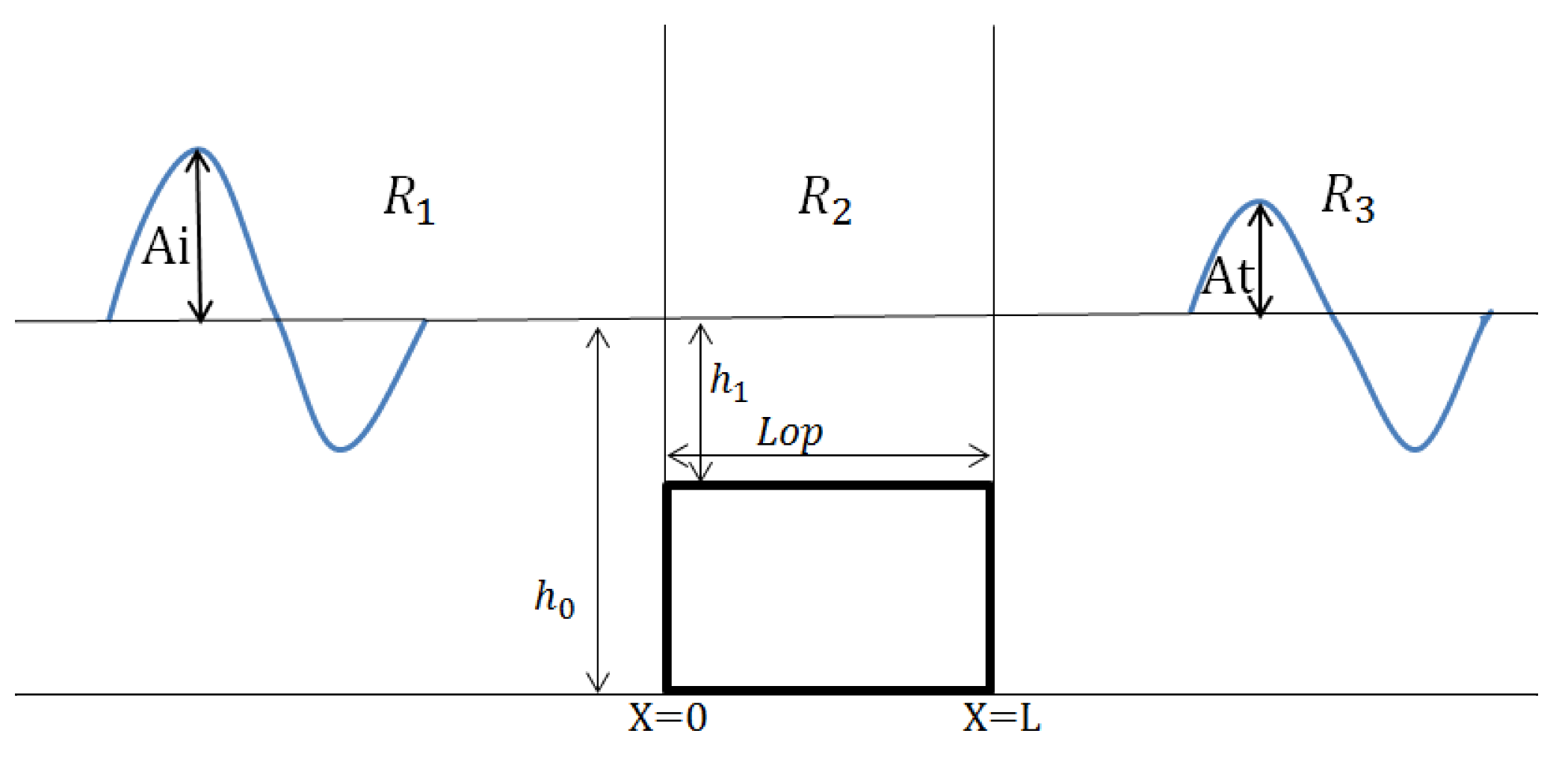
We use the Shallow Water Equations (SWEs) as our mathematical model. To visualize these equations, we consider an illustration of our problem, as shown in Figure 1.

As seen in Figure 1, $\eta (x,t)$ denotes the surface elevation, calculated from the undisturbed water level $z=0$. We use the symbol $u(x,t)$ for the horizontal component of water velocity, $d\left(x\right)$ for the bottom topography and $h(x,t)=\eta (x,t)+d\left(x\right)$ for the total water thickness. The system of linear SWEs over a bottom with depth $h\left(x\right)$ is given by

$${\eta }_t+{\left(hu\right)}_x=0,$$

(1)

$$u_t+g{\eta }_x=0,$$

(2)

where $g=9.81$ m/s², the gravity acceleration. The total depth h is defined by

$$h\left(x\right)=\left\{\begin{array}{cc}{h}_1,\hfill & \mathrm{for}0<x<L,\hfill \\ h_0,\hfill & elsewhere.\hfill \end{array}\right.$$

(3)

In this paper, we shall study the model for various parameters of the system depending on:

• Incoming wave amplitude,
• Incoming wave period,
• Breakwater height ($h_0-h_1$),
• Breakwater length,
• Water depth.

For a single breakwater system, we must consider three regions of our observation domain. These regions are $R_1:x<0$, $R_2:0<x<L$, $R_3:x>L$ as illustrated in Figure 2. We divide these regions based on how waves in each region behave. The behavior of waves is affected by the shape of the seafloor, which changes due to the existence of the breakwater.

3. Analytical Solution

In this section, we solve for the wave elevation and wave speed analytically from the SWEs using separation of variables. For this case, we consider a harmonic wave with frequency $\omega$ given by the equations

$$\eta (x,t)=F\left(x\right)e^{-i\omega t},$$

(4)

$$u(x,t)=G\left(x\right)e^{-i\omega t}.$$

(5)

where $F\left(x\right)$ and $G\left(x\right)$ are functions of x. We derive the solution for $\eta$ and u in each domain.

Region 1:

For $R_1$, we have the following equations

$${\eta }_1(x,t)=F_1\left(x\right)e^{-i\omega t},$$

(6)

$$u_1(x,t)=G_1\left(x\right)e^{-i\omega t},$$

(7)

Substituting Equations (6) and (7) in Equation (1), we obtain the relation

$$F_1\left(x\right)=\frac{h_0}{i\omega }{G}_1^{\prime }\left(x\right).$$

(8)

Similarly, substituting Equations (6) and (7) in (2), yields the relation

$$G_1\left(x\right)=\frac{g}{i\omega }{F}_1^{\prime }\left(x\right)$$

(9)

which implies that

$$G_1^{\prime }\left(x\right)=\frac{g}{i\omega }{F}_1^{″}\left(x\right).$$

(10)

Using the above expression for $G_1^{\prime }\left(x\right)$ in Equation (8), we obtain the following second order ordinary differential equation

$$F_1^{″}\left(x\right)+\frac{w^2}{g{h}_0}{F}_1\left(x\right)=0.$$

(11)

If we let $F_1\left(x\right)=e^{rx}$, the characteristic equation for Equation (11) is given by

$$r^2+\frac{w^2}{g{h}_0}=0$$

(12)

which gives the solution

$$F_1\left(x\right)=A_i{e}^{(\frac{w}{\sqrt{g{h}_0}}ix)}+A_r{e}^{(-\frac{w}{\sqrt{g{h}_0}}ix)}.$$

(13)

Hence, the analytical wave elevation in $R_1$ is

$$\begin{array}{ccc}\hfill {\eta }_1(x,t)& =& (A_i{e}^{(\frac{w}{\sqrt{g{h}_0}}ix)}+A_r{e}^{(-\frac{w}{\sqrt{g{h}_0}}ix)})e^{i\omega t}\hfill \\ \hfill & =& A_i{e}^{(\frac{w}{\sqrt{g{h}_0}}x-\omega t)i}+A_r{e}^{(-\frac{w}{\sqrt{g{h}_0}}x-\omega t)i}\hfill \end{array}$$

(14)

and the corresponding wave speed in $R_1$ is

$$u_1(x,t)=\sqrt{\frac{g}{h_0}}(A_i{e}^{(\frac{w}{\sqrt{g{h}_0}}x-\omega t)i}-A_r{e}^{(-\frac{w}{\sqrt{g{h}_0}}x-\omega t)i}).$$

(15)

Region 2:

Using a similar technique as in Region 1, we obtain these equations for $R_2$

$${\eta }_2(x,t)=F_2\left(x\right)e^{-i\omega t},$$

(16)

$$u_2(x,t)=G_2\left(x\right)e^{-i\omega t}.$$

(17)

Substituting Equations (16) and (17) in (1), we obtain

$$F_2\left(x\right)=\frac{h_1}{i\omega }{G}_2^{\prime }\left(x\right).$$

(18)

Then by substituting Equations (16) and (17) in Equation (2), we have

$$G_2^{\prime }\left(x\right)=\frac{g}{i\omega }{F}_2^{″}\left(x\right).$$

(19)

Replacing the value of $G_2^{\prime }\left(x\right)$ in Equation (18) with the result from Equation (19) yields:

$$F_2^{″}\left(x\right)+\frac{w^2}{g{h}_1}{F}_2\left(x\right)=0.$$

(20)

Letting $F_1\left(x\right)=e^{rx}$ gives the characteristic equation for (20):

$$r^2+\frac{w^2}{g{h}_1}=0.$$

(21)

This gives

$$F_2\left(x\right)=a{e}^{(\frac{w}{\sqrt{g{h}_1}}ix)}+b{e}^{(-\frac{w}{\sqrt{g{h}_1}}ix)}.$$

(22)

So, for $R_2$ we have

$$\begin{array}{ccc}\hfill {\eta }_2(x,t)& =& (a{e}^{(\frac{w}{\sqrt{g{h}_1}}ix)}+b{e}^{(-\frac{w}{\sqrt{g{h}_1}}ix)})e^{-i\omega t}\hfill \\ \hfill & =& a{e}^{(\frac{w}{\sqrt{g{h}_1}}x-\omega t)i}+b{e}^{(-\frac{w}{\sqrt{g{h}_1}}x-\omega t)i}\hfill \end{array}$$

(23)

with the following wave speed:

$$u_2(x,t)=\sqrt{\frac{g}{h_1}}(a{e}^{(\frac{w}{\sqrt{g{h}_0}}x-\omega t)i}-b{e}^{(-\frac{w}{\sqrt{g{h}_0}}x-\omega t)i}).$$

(24)

Region 3:

For $R_3$ we only have waves moving to the right. Therefore, $A_r=0$. Thus, we can assume that the wave elevation in $R_3$ is

$${\eta }_3(x,t)=A_t{e}^{(\frac{w}{\sqrt{g{h}_0}}(x-L)-\omega t)i},x>L$$

(25)

where $A_t$ is the transmitted wave amplitude. Thus, we can solve for the wave speed in $R_3$ by substituting Equation (25) in Equation (1). We obtain

$$u_3(x,t)=\sqrt{\frac{g}{h_0}}{A}_t{e}^{(\frac{w}{\sqrt{g{h}_0}}(x-L)-\omega t)i}.$$

(26)

In order to have continuous and smooth functions, we ensure the following conditions are fulfilled:

$${\eta }_1(0,t)={\eta }_2(0,t),h_0{u}_1(0,t)=h_1{u}_2(0,t)$$

(27)

and

$${\eta }_2(L,t)={\eta }_3(L,t),h_1{u}_2(L,t)=h_0{u}_3(L,t)$$

(28)

By solving the above system of equations, we obtain the transmission coefficient $K_t$ from

$$\frac{A_t}{A_i}=\frac{4\sqrt{\frac{h_0}{h_1}}}{{(1+\sqrt{\frac{h_0}{h_1}})}^2{e}^{(-\frac{w}{\sqrt{g{h}_1}}iL)}-{(1-\sqrt{\frac{h_0}{h_1}})}^2{e}^{(\frac{w}{\sqrt{g{h}_1}}iL)}}$$

(29)

Thus, the transmission coefficient is given by

$$K_t=|\frac{A_t}{A_i}|=\frac{4\sqrt{\frac{h_0}{h_1}}}{|4\sqrt{\frac{h_0}{h_1}}cos(\frac{w}{\sqrt{g{h}_1}}L)-2isin(\frac{w}{\sqrt{g{h}_1}}L)-2\frac{h_0}{h_1}isin(\frac{w}{\sqrt{g{h}_1}}L)|}.$$

(30)

Notice that this function depends only on $h_0$, $h_1$, and L. By squaring $K_t$, we obtain

$${\left(K_t\right)}^2=\frac{16\frac{h_0}{h_1}}{4{(1+\frac{h_0}{h_1})}^2{sin}^2(\frac{w}{\sqrt{g{h}_1}}L)+16\frac{h_0}{h_1}{cos}^2(\frac{w}{\sqrt{g{h}_1}}L).}$$

(31)

To find the breakwater length that reduces the amplitudes of incoming waves optimally, we determine the smallest possible value of $K_t$. From Equation (31), we minimize the value of $K_t$ by letting $si{n}^2(\frac{w}{\sqrt{g{h}_1}}L)=1$ and $co{s}^2(\frac{w}{\sqrt{g{h}_1}}L)=0$, so we get

$$\frac{w}{\sqrt{g{h}_1}}L=\frac{\pi }{2}+2k\pi ,k=0,1,2,3,\dots$$

(32)

Then we have $L_{opt}=\frac{(\frac{\pi }{2}+2k\pi )\sqrt{g{h}_1}}{w}$. To maximize breakwater length efficiency, we choose $k=0$. Thus, we have the optimal amplitude-reducing breakwater length

$$L_{opt}=\frac{\pi \sqrt{g{h}_1}}{2w}.$$

(33)

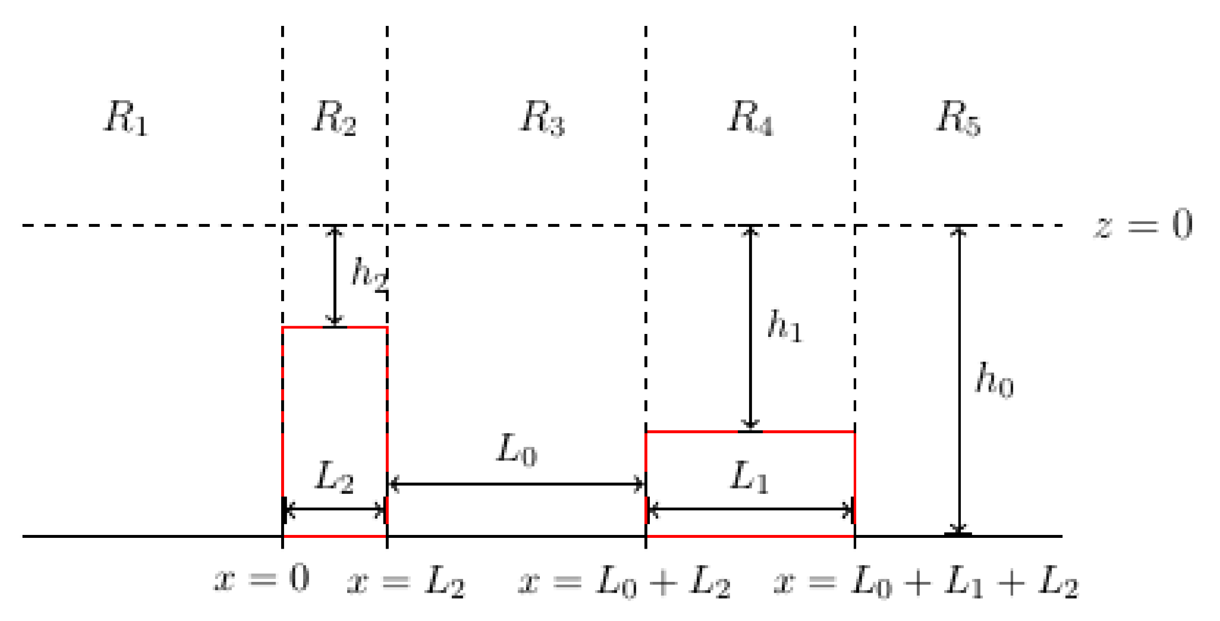
4. The Two-Bar Wave Reflector Problem and Its Generalization

In this section, we generalize the preceding results to n-submerged bars. First, let us consider a two-bar wave reflector that is made up of two identical bars with height $(h_0-h_1)$, length $L_1$ and separated by a distance $L_0$. In this case, the bottom topography is given by

$$h\left(x\right)=\left\{\begin{array}{c}{h}_1\mathrm{for}\left(0<x<L_1\right)\cup \left(L_0+L_1<x<L_0+2L_1\right)\hfill \\ h_0\mathrm{elsewhere}.\hfill \end{array}\right.$$

(34)

The bottom topography described by Equation (34) is illustrated in Figure 3.

Similar to the one-bar wave reflector case, we assume that the governing equation is the linear SWEs and the solution for the system of this equations are

$$\begin{array}{ccc}\hfill {\eta }_j(x,t)& =& F_j\left(x\right)e^{-i\omega t}\hfill \end{array}$$

(35)

$$\begin{array}{ccc}\hfill u_j(x,t)& =& G_j\left(x\right)e^{-i\omega t},\hfill \end{array}$$

(36)

for $j=1,2,3,4,5$ which corresponds to each region $R_j$.

Table 1. Surface elevation $\eta (x,t)$ and water velocity $u(x,t)$ of an incident wave.

Region	Solution for $\mathit{\eta }(\mathit{x},\mathit{t})$	Solution for $\mathit{u}(\mathit{x},\mathit{t})$
$R_1$	$A_{i}exp(i{k}_{0}x-i\omega t)+A_{r}exp(-i{k}_{0}x-i\omega t)$	${\displaystyle \sqrt{\frac{g}{h_0}}\left(A_{i}exp(i{k}_{0}x-i\omega t)-A_{r}exp(-i{k}_{0}x-i\omega t)\right)}$
$R_2$	$a_{1}exp(i{k}_{1}x-i\omega t)+b_{1}exp(-i{k}_{1}x-i\omega t)$	${\displaystyle \sqrt{\frac{g}{h_1}}\left(a_{1}exp(i{k}_{1}x-i\omega t)-b_{1}exp(-i{k}_{1}x-i\omega t)\right)}$
$R_3$	$a_{2}exp(i{k}_{0}x-i\omega t)+b_{2}exp(-i{k}_{0}x-i\omega t)$	${\displaystyle \sqrt{\frac{g}{h_0}}\left(a_{2}exp(i{k}_{0}x-i\omega t)-b_{2}exp(-i{k}_{0}x-i\omega t)\right)}$
$R_4$	$a_{3}exp(i{k}_{1}x-i\omega t)+b_{3}exp(-i{k}_{1}x-i\omega t)$	${\displaystyle \sqrt{\frac{g}{h_1}}\left(a_{3}exp(i{k}_{1}x-i\omega t)-b_{3}exp(-i{k}_{1}x-i\omega t)\right)}$
$R_5$	$A_{t}exp(i{k}_0(x-2L_1-L_0)-i\omega t)$	${\displaystyle \sqrt{\frac{g}{h_0}}{A}_{t}exp(i{k}_0(x-2L_1-L_0)-i\omega t)}$

summarizes the result of a lengthy calculation for ${\eta }_j$ and $u_j$ (similar to the one-bar case) for each region $R_j$.

In the above table, $A_r,A_t,a_k,\mathrm{and}{b}_k$, $k=1,2,3$ are undetermined coefficients. It was argued by Pudjaprasetya et al. [29] that the optimal length $L_1$ of the bar is equal to one-fourth of the wavelength ${\displaystyle {\lambda }_1=\frac{2\pi \sqrt{g{h}_1}}{\omega }}$ and the optimal distance between such bars is one-fourth of the wavelength ${\lambda }_0$ given by ${\displaystyle \frac{2\pi \sqrt{g{h}_0}}{\omega }}$ because destructive interference happens when such conditions are satisfied. Now, to determine how effective a two-bar wave reflector is, we compute its transmission and reflection coefficients. We do so by equating ${\eta }_j$ and ${\eta }_{j+1}$ (for $j=1,2,3,4$) and $h_0{u}_j=h_1{u}_{j+1}$ (for $j=1,3$) or $h_1{u}_j=h_0{u}_{j+1}$ (for $j=2,4$) at each point of discontinuity. Calculating, we get

$${\displaystyle \left|\frac{A_t}{A_i}\right|=\frac{4|a^2-b^2|}{\left|\mathsf{\Delta }\right|},}$$

(37)

where

$$\begin{array}{cc}\hfill \mathsf{\Delta }=& a^{3}cexp(-i{k}_0{L}_0-2i{k}_1{L}_1)+a^{2}bdexp(-i{k}_0{L}_0)+a^{2}bdexp(i{k}_0{L}_0-2i{k}_1{L}_1)\hfill \\ \hfill & +a{b}^{2}cexp\left(i{k}_0{L}_0\right)+a{b}^{2}cexp(-i{k}_0{L}_0)+b^{3}dexp(-i{k}_0{L}_0+2i{k}_1{L}_1)\hfill \\ \hfill & +a^{2}bdexp\left(i{k}_0{L}_0\right)+a{b}^{2}cexp(i{k}_0{L}_0+2i{k}_1{L}_1)\hfill \end{array}$$

(38)

and

$${\displaystyle a=1+\sqrt{\frac{h_0}{h_1}},b=1-\sqrt{\frac{h_0}{h_1}},c=1+\sqrt{\frac{h_1}{h_0}},\mathrm{and}d=1-\sqrt{\frac{h_1}{h_0}}.}$$

(39)

Similarly, the reflection coefficient is given by

$${\displaystyle \left|\frac{A_r}{A_i}\right|=\frac{\left|\alpha \right|}{\left|\beta \right|}}$$

(40)

where

$$\begin{array}{cc}\hfill \alpha =& a^{2}cdexp(i{k}_0{L}_0+2i{k}_1{L}_1)+ab{d}^{2}exp\left(i{k}_0{L}_0\right)+ab{d}^{2}exp(-i{k}_0{L}_0+2i{k}_1{L}_1)\hfill \\ \hfill & +b^{2}cdexp(-i{k}_0{L}_0)+ab{c}^{2}exp\left(i{k}_0{L}_0\right)+b^{2}cdexp(i{k}_0{L}_0-2i{k}_1{L}_1)\hfill \\ \hfill & +a^{2}cdexp(-i{k}_0{L}_0)+ab{c}^{2}exp\left(-i{k}_0{L}_0-2i{k}_1{L}_1\right)\hfill \end{array}$$

(41)

and

$$\begin{array}{cc}\hfill \beta =& abcdexp(i{k}_0{L}_0+2i{k}_1{L}_1)+a^2{d}^{2}exp\left(i{k}_0{L}_0\right)+b^2{d}^{2}exp(-i{k}_0{L}_0+2i{k}_1{L}_1)\hfill \\ \hfill & +abcdexp(-i{k}_0{L}_0)+b^2{c}^{2}exp\left(i{k}_0{L}_0\right)+abcdexp(i{k}_0{L}_0-2i{k}_1{L}_1)\hfill \\ \hfill & +abcdexp(-i{k}_0{L}_0)+a^2{c}^{2}exp(-i{k}_0{L}_0-2i{k}_1{L}_1)\hfill \end{array}$$

(42)

where $a,b,c,\mathrm{and}d$ are given as above. Again, we can show that $|A_t{|}^2+|A_r{|}^2={\left|A_i\right|}^2$, which indicates that the energy is conserved.

An interesting property of the transmission coefficient function for a two-bar wave reflector, which we will denote by $K_t^2$, and its corresponding reflection coefficient function $K_r^2$ is stated in the following theorem:

Theorem 1.

The transmission coefficient $K_t^2$ and reflection coefficient $K_r^2$ for a two-bar wave reflector with optimal dimension $(h_0-h_1)\times L_1$ separated by a distance $L_0$, where $L_i={\displaystyle \frac{\pi \sqrt{g{h}_i}}{2\omega }}$, $i=0,1$, placed on a flat bottom topography and submerged in water with depth $h_0$ are given by

$$K_t^2\left(x\right)=K_t\left(x^2\right)\mathrm{and}{K}_r^2\left(x\right)=K_r\left(x^2\right),\forall x\ge 1.$$

(43)

Proof. 

The proof of the theorem follows immediately from our computations after substituting $L_0$ and $L_1$ in Equations (37) and (40). □

Hence, we do not actually need to work with each matching condition just to find the transmission and reflection coefficient for a two-bar wave reflector given its optimal dimension (length and separation distance). This interesting property can be generalized to the case of n bars. We have the following theorem:

Theorem 2.

The transmission coefficient $K_t^n$ and reflection coefficient $K_r^n$ for an n-bar wave reflector with optimal dimension $(h_0-h_1)\times L_1$ separated by a distance $L_0$, where $L_i={\displaystyle \frac{\pi \sqrt{g{h}_i}}{2\omega }}$, $i=0,1$, placed on a flat bottom topography and submerged in water with depth $h_0$ are given by

$$\begin{array}{ccc}\hfill K_t^n\left(x\right)& =& K_t\left(x^n\right),\hfill \end{array}$$

(44)

$$\begin{array}{ccc}\hfill K_r^n\left(x\right)& =& K_r\left(x^n\right),\hfill \end{array}$$

(45)

for all $x\ge 1$.

Proof. 

We proceed by induction.

Base step: For $n=1,2$, we have already shown above that Equations (44) and (45) hold.

Inductive step: Suppose Equations (44) and (45) hold for $n=m\in \mathbb{N}$. This means that there exists a one-bar wave reflector with height $(h_0-h_2)$ and length $L_2$ corresponding to the m-bar wave reflector each with dimension $(h_0-h_1)\times L_1$. In particular, we take $h_2=h_1^m{h}_0^{1-m}$. Now, we have to show that the formulas hold for $n=m+1$. We ‘group’ the m-bar wave reflector into a one-bar wave reflector and then form a two-bar wave reflector with a one-bar reflector with the same dimension as the m-bar reflector (refer to Figure 4.) Hence, our problem is now reduced to a two-bar wave reflector problem with non-identical bars.

Like the one-bar wave reflector case, we assume that the governing equation is the linear SWEs and the solution for the system of equations is given by

$$\begin{array}{ccc}\hfill {\eta }_j(x,t)& =& F_j\left(x\right)e^{-i\omega t}\hfill \end{array}$$

(46)

$$\begin{array}{ccc}\hfill u_j(x,t)& =& G_j\left(x\right)e^{-i\omega t},\hfill \end{array}$$

(47)

for $j=1,2,3,4,5$, which corresponds to each region $R_j$.

Table 2. Surface elevation $\eta (x,t)$ and water velocity $u(x,t)$ of an incident wave.

Region	Solution for $\mathit{\eta }(\mathit{x},\mathit{t})$	Solution for $\mathit{u}(\mathit{x},\mathit{t})$
$R_1$	$A_{i}exp(i{k}_{0}x-i\omega t)+A_{r}exp(-i{k}_{0}x-i\omega t)$	${\displaystyle \sqrt{\frac{g}{h_0}}\left(A_{i}exp(i{k}_{0}x-i\omega t)-A_{r}exp(-i{k}_{0}x-i\omega t)\right)}$
$R_2$	$a_{1}exp(i{k}_{2}x-i\omega t)+b_{1}exp(-i{k}_{2}x-i\omega t)$	${\displaystyle \sqrt{\frac{g}{h_2}}\left(a_{1}exp(i{k}_{2}x-i\omega t)-b_{1}exp(-i{k}_{2}x-i\omega t)\right)}$
$R_3$	$a_{2}exp(i{k}_{0}x-i\omega t)+b_{2}exp(-i{k}_{0}x-i\omega t)$	${\displaystyle \sqrt{\frac{g}{h_0}}\left(a_{2}exp(i{k}_{0}x-i\omega t)-b_{2}exp(-i{k}_{0}x-i\omega t)\right)}$
$R_4$	$a_{3}exp(i{k}_{1}x-i\omega t)+b_{3}exp(-i{k}_{1}x-i\omega t)$	${\displaystyle \sqrt{\frac{g}{h_1}}\left(a_{3}exp(i{k}_{1}x-i\omega t)-b_{3}exp(-i{k}_{1}x-i\omega t)\right)}$
$R_5$	$A_{t}exp(i{k}_0(x-L_0-L_1-L_2)-i\omega t)$	${\displaystyle \sqrt{\frac{g}{h_0}}{A}_{t}exp(i{k}_0(x-L_0-L_1-L_2)-i\omega t)}$

below summarizes the result of a lengthy calculation for ${\eta }_j$ and $u_j$ for each region $R_j$.

Equating $\eta$ and $hu$ for each pair of adjacent regions, we obtain

$$\begin{array}{cc}\hfill \left|\frac{A_t}{A_i}\right|=& 16|\{a_1{b}_1{c}_1{d}_1(1/p)(1/q)(1/r)+a_1{b}_1{c}_2{d}_2(1/p)q(1/r)+\hfill \\ \hfill & a_1{b}_2{c}_2{d}_{1}p(1/q)(1/r)+a_1{b}_2{c}_1{d}_{2}pq(1/r)+\hfill \\ \hfill & a_2{b}_2{c}_1{d}_1(1/p)(1/q)r+a_2{b}_2{c}_2{d}_2(1/p)qr+\hfill \\ \hfill & a_2{b}_1{c}_2{d}_{1}p(1/q)r+a_2{b}_1{c}_1{d}_2{pqr\}}^{-1}|\hfill \end{array}$$

(48)

and

$$\begin{array}{c}\hfill \left|{\displaystyle \frac{A_r}{A_i}}\right|={\displaystyle \frac{\left|\alpha \right|}{\left|\beta \right|}}\end{array}$$

(49)

where

$$\begin{array}{c}{a}_1=1+\sqrt{h_2/h_0}{a}_2=1-\sqrt{h_2/h_0}p=expi{k}_0{L}_0\\ b_1=1+\sqrt{h_0/h_2}{b}_2=1-\sqrt{h_0/h_2}q=expi{k}_1{L}_1\\ c_1=1+\sqrt{h_1/h_0}{c}_2=1-\sqrt{h_1/h_0}r=expi{k}_2{L}_2\\ d_1=1+\sqrt{h_0/h_1}{d}_2=1-\sqrt{h_0/h_1}\end{array}$$

(50)

and

$$\begin{array}{cc}\hfill \alpha =& c_2{d}_1{a}_1{b}_{1}pqr+c_2{d}_1{a}_2{b}_{2}pq(1/r)+c_2{d}_2{a}_2{b}_1(1/p)qr+\hfill \\ \hfill & c_2{d}_2{a}_1{b}_2(1/p)q(1/r)+c_1{d}_2{a}_1{b}_{1}p(1/q)r+c_1{d}_2{a}_2{b}_{2}p(1/q)(1/r)+\hfill \\ \hfill & c_1{d}_1{a}_2{b}_1(1/p)(1/q)r+c_1{d}_1{a}_1{b}_2(1/p)(1/q)(1/r),\hfill \end{array}$$

(51)

$$\begin{array}{cc}\hfill \beta =& c_2{d}_1{a}_1{b}_{2}pqr+c_2{d}_1{a}_2{b}_{1}pq(1/r)+c_2{d}_2{a}_2{b}_2(1/p)qr+\hfill \\ \hfill & c_2{d}_2{a}_1{b}_1(1/p)q(1/r)+c_1{d}_2{a}_1{b}_{2}p(1/q)r+c_1{d}_2{a}_2{b}_{1}p(1/q)(1/r)+\hfill \\ \hfill & c_1{d}_1{a}_2{b}_2(1/p)(1/q)r+c_1{d}_1{a}_1{b}_1(1/p)(1/q)(1/r).\hfill \end{array}$$

(52)

Upon substitution of $L_i={\displaystyle \frac{\pi \sqrt{g{h}_i}}{2\omega }}$, $i=0,1,2$, we indeed obtain Equations (44) and (45) for $n=m+1$. □

Notice that we set our domain for the functions $K_t^n$ and $K_r^n$ to be $[1,+\infty )$ because from our calculations, these functions admit values of $\sqrt{h_0/h_1}\ge 1$. As an immediate consequence of our formulas, we can find a series of identical n-bar wave reflector of height $\left(h_0-h_1^n{h}_0^{1-n}\right)$ that is equally effective in terms of transmission and reflection to a one-bar wave reflector with height $(h_0-h_1)$. For example, a two-bar wave reflector with height $0.6h_0$ is equally effective with a one-bar wave reflector each with height $0.84h_0$. It can be concluded that energy is also conserved for this type of wave reflector. We can try to do the lengthy computation (e.g., for the three-bar wave reflector case, we can set-up the 12 matching conditions just to find $K_t^3$ and $K_r^3$). However, with the aid of a computer software, we can just set-up the matrix equation

$$\mathbf{Ax}=\mathbf{b}$$

(53)

where ${\mathbf{A}}_{4n\times 4n}$ is the coefficient matrix and $\mathbf{b}={\left[\begin{array}{ccc}1& 1& 0\cdots 0\end{array}\right]}_{1\times 4n}^T$ and n is the number of identical parallel bars. Finally, we note that in the solution vector $\mathbf{x}$, $x_1=A_r$ and $x_{4n}=A_t$.

5. Numerical Method

We now solve Equations (1) and (2) numerically using the finite volume method on a staggered grid. The finite volume method is one of the known numerical methods for solving partial differential equations (see [30] for details of the method). We will define the scheme to simulate wave propagation and see what happens to the wave that passes through the breakwater and how effective the breakwater is on reducing wave amplitude. Furthermore, we investigate the wave when it passes through a domain with various system conditions. We base these system conditions on varying incoming wave amplitude, wave period, water depth, breakwater length, and breakwater height. Figure 5 below illustrates how the staggered grid works. In the staggered grid arrangement, the value of $\eta$ is calculated on a full grid and u is calculated on a half grid.

Mass conservation (Equation (1)) is approximated at a cell centered at $x_i$, while momentum conservation (Equation (2)) is approximated at a cell centered at $x_{i+1/2}$. Afterward, we discretize Equations (1) and (2) and approximate them using the numerical equations below, which are based on the finite volume method on a staggered grid:

$$\frac{{\eta }_j^{n+1}-{\eta }_j^n}{\mathsf{\Delta }t}+\frac{{\left(hu\right)}_{j+1/2}^n-{\left(hu\right)}_{j-1/2}^n}{\mathsf{\Delta }x}=0$$

(54)

$$\frac{u_{j+1/2}^{n+1}-u_{j+1/2}^n}{\mathsf{\Delta }t}+g\frac{{\eta }_{j+1}^{n+1}-{\eta }_j^{n+1}}{\mathsf{\Delta }x}=0$$

(55)

In this case, the values of water elevation $\eta$ will be computed at every full grid point $x_i$, with $i=1,2,3,...,Nx$ using mass conservation (Equation (54)). Velocity u will be computed at every staggered grid point $x_{i+1/2}$, with $i=0,1,2,\dots ,Nx$ using momentum conservation (Equation (55)). Using Von Neumann’s stability analysis, we obtain the Courant–Friedrichs–Lewy condition for Equations (54) and (55), which is $\sqrt{g{h}_1}\frac{\mathsf{\Delta }t}{\mathsf{\Delta }x}\le 1$.

6. Results and Discussion

In this section, we will implement the numerical scheme that has been formulated in the previous section to simulate wave propagation over rectangular submerged breakwater. Further, we will compare the numerical results with the analytical solutions, literature data, and experimental measurements to validate the scheme.

6.1. Wave Propagation over a Submerged Breakwater

Here, we simulate the wave propagation over a rectangular breakwater using the numerical scheme of Equations (54) and (55) from the previous section. We will simulate the wave in three states: before it encounters the breakwater, as it passes above the breakwater, and after it passes through the breakwater. We do this by defining the value of h in each region. For the region behind the breakwater and in front of the breakwater, we take the value of $h=h_0$ as the water depth from the undisturbed wave surface to the bottom. For Region 2, where the breakwater exists, we take $h=h_1$ as the distance between the top of the breakwater and the undisturbed wave surface.

The incoming wave is modeled using the sinusoidal function with specific wave amplitudes and periods. The numerical $K_t$ is calculated by determining the ratio of the maximum value of $\eta$ in region 3 at the end of wave iteration to the generated incoming wave amplitude $A_i$. Below is an example of a numerical model simulation (Figure 6).

We obtained $K_t=0.9393$ from our numerical model, meaning that the incoming wave amplitude is reduced by $0.0607$ or about six percent. Notice that the simulation example gives us $K_t<1$, which means that the breakwater is effective in reducing relatively small wave amplitudes. However, a relatively high value of $K_t$ means that the breakwater may increase the wave amplitude instead of reducing it, and its existence could be harmful to structures near the shoreline.

Now, we will conduct another simulation for wave propagation over a submerged rectangular breakwater using our numerical scheme. The results will then be compared to the numerical results obtained by Rambabu and Mani [31] to confirm our model. In this case, the ratio between the length of the breakwater $\left(L\right)$ and the water depth $\left(h_0\right)$ is set to be $L/h_0=1$, while the ratio between the depth on top of the breakwater and on the deeper bottom is $h_1/h_0=0.2$. Using both models, the values of $K_t$ are calculated for different values of $kd$. Figure 7 presents the comparison between the $K_t$ obtained using our model and using the model proposed by Rambabu and Mani [31]. The comparison gives a very good agreement where our model confirms the model in [31] perfectly.

6.2. Validation with Analytical Solution

Next, we will validate our numerical scheme by comparing the results against the analytical solutions obtained from Section 3. Figure 8 shows the comparison between numerical results and analytical solutions for the value of $K_t$ and $K_r$ for various $\sqrt{h_0/h_1}$. In this case, we set the water depth without breakwater as $h_0$ = 10 m, while the depth on top of the crest is varied.

From Figure 8, we can investigate further the transmission and reflection coefficient, especially how the depth of the breakwater’s crest affects the value of $K_t$ and $K_r$. Note that by making the value $\sqrt{h_0/h_1}$ larger, the value of $K_t$ will be smaller, $K_r$ becomes larger. From this, we can conclude that by increasing the breakwater’s height, we also increase the efficiency of the breakwater itself. However, keep in mind that building high breakwaters may cost more. From this result, we can calculate the breakwater’s height to fit the needs of its structure as well as its budget.

Now, there is one more factor that could significantly affect the transmission and reflection coefficient: the length of the breakwater. Figure 9 illustrates the changes in the value of $K_t$ and $K_r$ affected by the changes in the breakwater’s length. The figure only shows the case for analytical $K_t$ and $K_r$. From the figure, we can see that the value of $K_t$ and $K_r$ are both affected by the length of the breakwater periodically, with the maximum value of $K_t=1$ and minimum value $K_r=0$. The results in the form of a periodic function mean that we can determine the optimum value of L. Analytically, we have determined in Section 3 that the optimal breakwater length for reducing the wave amplitude is given as follows:

$$L_{opt}=\frac{\pi \sqrt{g{h}_1}}{2\omega }.$$

(56)

Furthermore, we want to see how effective the submerged breakwater is in reducing wave amplitude if we use the optimal length. Figure 10 shows a plot of the $K_t$ value when $L_{opt}$ and other values of L are used. It can be inferred from this plot that the value of $K_t$ when the breakwater has an optimal length will always be smaller than the values of $K_t$ for other L. This means that our equation for $L_{opt}$ is physically correct. Therefore, it can be concluded that when the submerged breakwater used is rectangular, we can select $L_{opt}$ as its length and set the breakwater height as high as possible while still keeping it underwater.

This model can be developed further by considering the wave reflected from the wave damper, which can also affect $K_t$. In addition, for further research, we can also take into account the wave damper’s influence on wave amplitude. Therefore, by using this numerical and analytical model, we can determine the optimal size of the breakwater on reducing the wave amplitude with results that are even closer to those obtained from experiments using a physical model. That means we can use this model instead of constructing expensive physical models in future research relevant to Linear Shallow Water Equations.

6.3. Validation with Experimental Data

In this subsection, we will compare the values of $K_t$ from our numerical simulations with the data collected from experiments involving physical models of submerged breakwaters. It is hoped that the error calculated from comparing these results will be small, so that we can use this numerical model to emulate the physical phenomenon of scattering waves due to the existence of a breakwater structure.

Experiments involving physical models of our system were carried out in the Indonesian Ministry of Public Works’ Coastal Research and Development Center, Buleleng-Bali, Indonesia. We set up the model and collected data. The results contain the transmission coefficients corresponding to each system scenario. Each system scenario is created by setting the breakwater length, breakwater height, water depth, wave height, and wave period. The wave channel has a length of 40 m, a width of 0.6 m and a height of 1.2 m. With variations of placement of structures on the wave channel, the model test area utilizes 34 m of space. The laboratory wave channel is equipped with a piston-type generator engine powered by an electric motor capable of generating regular waves up to a height of 25 cm with a period of 1–2.6 s. The wave channel also has wave probes behind and in front of the breakwater, allowing us to gather information on wave amplitudes before and after waves pass through the breakwater. A pile of hollow stone mounted on the wave channel acts as a wave damper. Figure 11 illustrates the physical model set-up used in the experiment. The various breakwater sizes used in the physical model are listed in

Table 3. List of various breakwater size that are used in the experiment.

Type No.	Height (H)	Length (L)
1	30 cm	45 cm
2	30 cm	30 cm
3	30 cm	15 cm
4	20 cm	45 cm
5	20 cm	30 cm
6	20 cm	15 cm

with water depth variations of 35, 40, 45, 50, and 60 cm.

We obtain $K_t$ values from the variations of the physical model that meet the linear SWEs assumptions for various breakwater sizes, water depths, wave heights, and wave periods. In

Table 4. Comparison between physical and numerical $K_t$ for various model scenarios.

No.	H (m)	A (m)	T (s)	${\mathit{h}}_0$ (cm)	BW (cm)	L (cm)	Physical ${\mathit{K}}_{\mathit{t}}$	Numerical ${\mathit{K}}_{\mathit{t}}$	Error (%)
1	0.10879	0.05439	1.61	60	30	30	0.8435	0.8870	5.15708
2	0.07156	0.03578	2.04	60	30	15	0.8580	0.8578	0.02331
3	0.06793	0.03396	2.04	60	20	15	0.9483	0.9209	2.88938
4	0.10757	0.05378	1.61	60	20	30	0.9687	0.9392	3.04532
5	0.19330	0.09665	1.08	60	20	45	0.8311	0.8770	5.53380
6	0.09281	0.04641	1.61	50	20	30	0.8899	0.9295	4.44994
7	0.05919	0.02959	2.04	50	20	15	0.9254	0.9047	2.23687
8	0.09060	0.04530	1.61	50	30	30	0.8442	0.8652	2.48756
9	0.04082	0.02041	2.04	45	20	15	1.0860	0.9890	8.93186
10	0.08762	0.04381	1.61	45	20	30	0.9539	0.9249	3.04015
11	0.09100	0.04550	1.61	45	30	30	0.8492	0.8462	0.35317
12	0.06249	0.03125	1.61	40	20	30	1.0339	0.9209	10.92949
13	0.05665	0.02833	2.04	35	20	15	0.8240	0.8649	4.96359
14	0.06912	0.03456	1.61	35	20	30	0.8591	0.9179	6.84437
15	0.11318	0.05659	1.08	35	20	45	0.9158	0.9528	4.04018

, H denotes the incoming wave height, A is the incoming wave amplitude (half of the wave height), T is the wave period in seconds, $h_0$ is the undisturbed water depth without breakwater, and $BW$ is the breakwater height. In order to analyze the effect of incoming wave amplitude, we use the wave amplitude in meter units. The experimental data, numerical results, and the relative error of our model can be seen in Table 4.

From the comparison above, with certain characteristics of wave amplitude, wave period, breakwater size, and water depth, the transmission coefficient values obtained using the numerical model have an average error of $4.2\%$ when compared to transmission coefficients obtained from the physical model data. For numerical mathematical modeling in general, this error is relatively small. Therefore, we can conclude that the model adequately simulates wave reduction.

7. Conclusions

In this paper, the linearized Shallow Water Equations is solved analytically and numerically using the Separation of Variables Method and Finite Volume Method on a Staggered Grid, respectively, to obtain the transmission coefficient ($K_t$). Analytically, we have found the solution for $K_t$ for single-bar and two-bar submerged breakwater, which strongly depend on the dimension of the breakwater itself. While the $K_t$ for a single-bar case only depends on the size of the bar, $K_t$ for a two-bar case also depends on the distance between the two bars. The generalized $K_t$ for an n-bar submerged breakwater is obtained using a theorem of which proof is presented in this paper. The higher the breakwater, the lower $K_t$ we get. Moreover, the optimal length of each bar $L_{opt}=\frac{\pi \sqrt{g{h}_1}}{2\omega }$ has also been obtained for specific incoming wave amplitudes. Moreover, solving the model numerically using the finite volume method on a staggered grid, resulted in a very accurate simulation where the wave amplitude is reduced after it passes the bar. To validate the numerical scheme, comparisons between our numerical results against previous numerical model results, analytical solutions, and experimental data have been conducted. The comparison between our numerical model against the previous numerical model based on the Potential Theory as well as the analytical-numerical comparison give almost identical results for both cases. Agreeing with those results, the comparison between our numerical results against the experimental data gives a very good agreement with only 4.2% of error, which is relatively small for the comparison. Those results indicate that our model is quite good at simulating the real phenomena, which is important because then we can use this research to provide a good preliminary design tool for the implementation of submerged breakwaters as a coastal protector.