Accurate Energy and Performance Prediction for Frequency-Scaled GPU Kernels


Abstract
1. Introduction
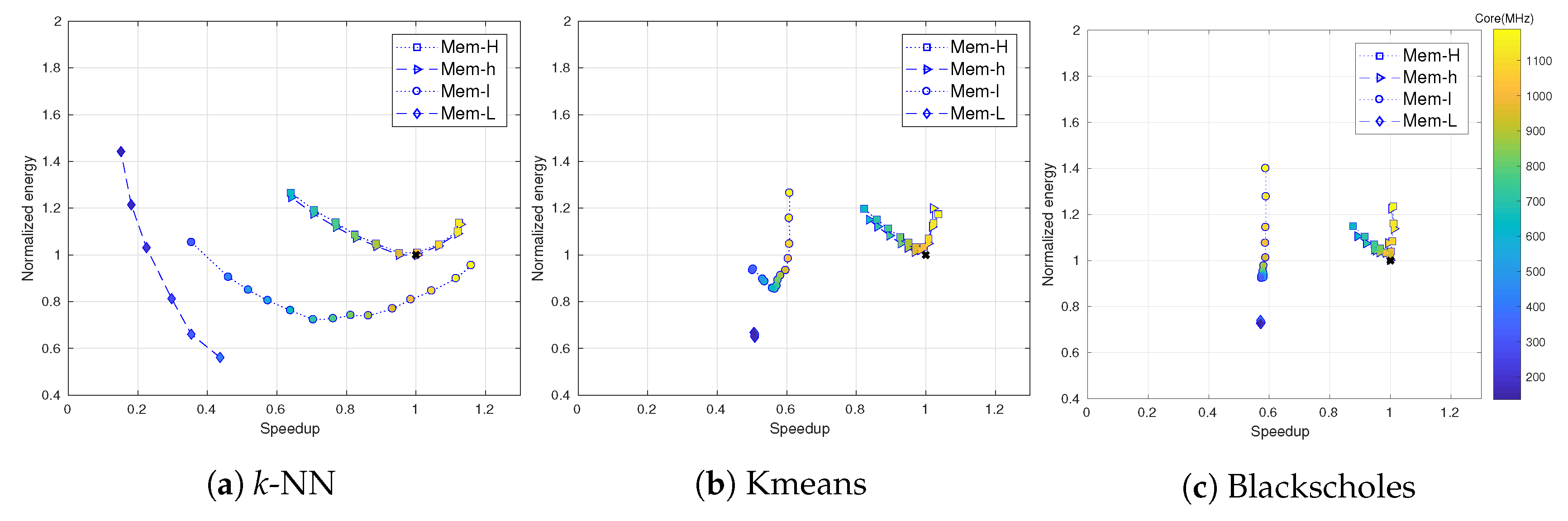
- An analysis of the Pareto optimality (performance versus energy consumption) of GPU applications on a multi-domain frequency scaling setting on an NVIDIA Titan X.
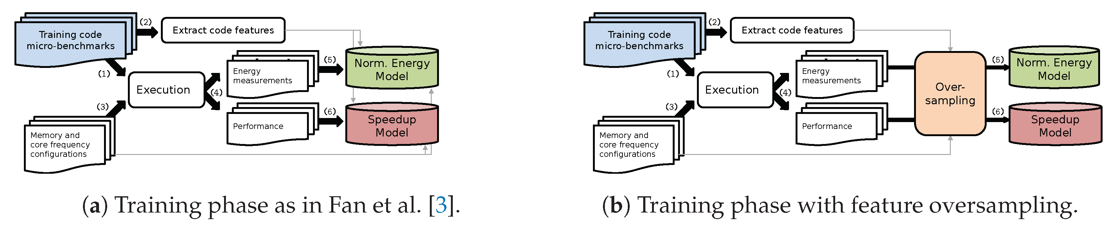
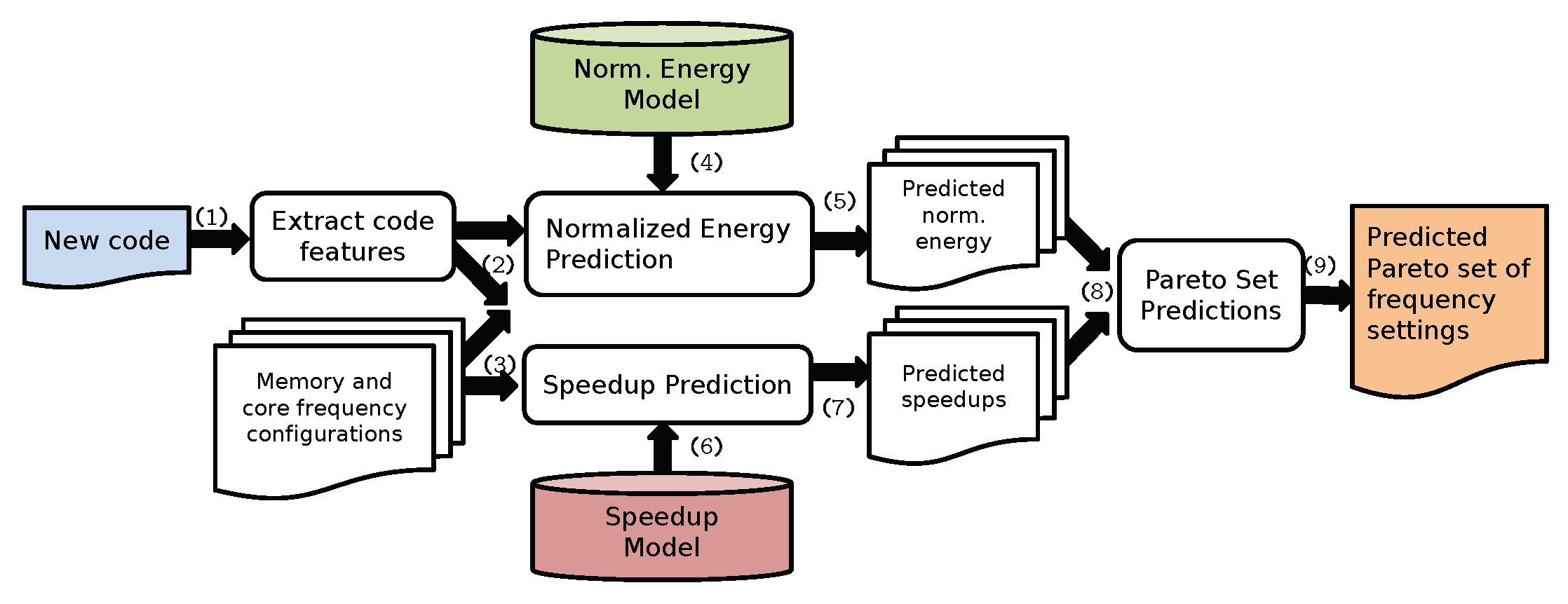
- A modeling approach based on static code features that predicts core and memory frequency configurations, which are Pareto-optimal with respect to energy and performance. The model was built on 106 synthetic micro-benchmarks. It predicts normalized energy and speedup with specific methods, and then derives a Pareto set of configurations out of the individual models.
- An experimental evaluation of the proposed models on an NVIDIA Titan X, and a comparison against the default static settings.
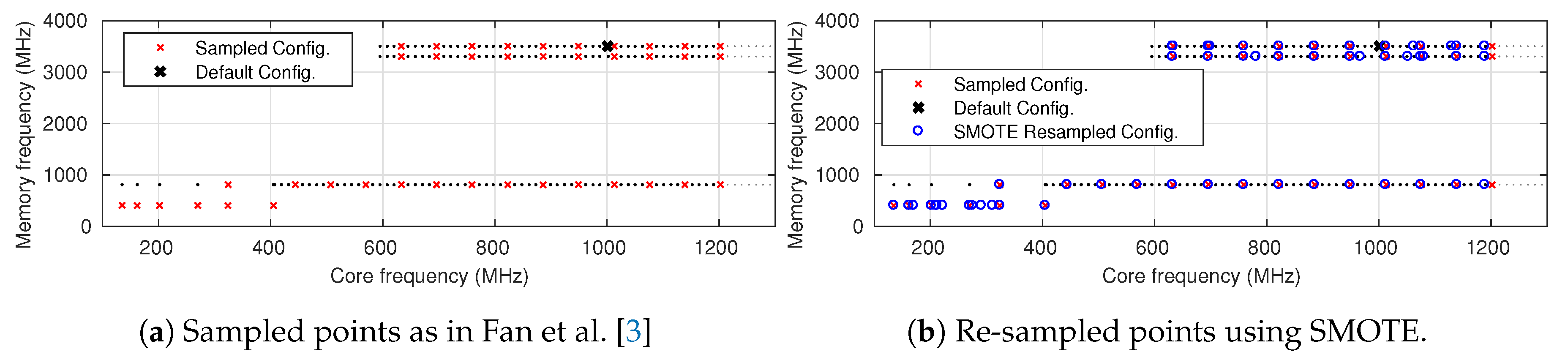
- A novel methodology for handling an imbalanced dataset based on the SMOTE algorithm, which further improves the modeling for critical cases; e.g., low memory frequency configurations.
- An analysis of the impacts of various input sizes on energy and performance.
- An extended analysis of the energy and performance application characterization on a set of twelve applications.
2. Related Work
3. Background
3.1. Overview
3.2. Features
3.3. Training Data
3.4. Predictive Modeling
3.4.1. Speedup Prediction
3.4.2. Normalized Energy Model
3.4.3. Deriving the Pareto Set
| Algorithm 1 Simple Pareto set calculation. |
|
4. Modeling Imbalanced Dataset
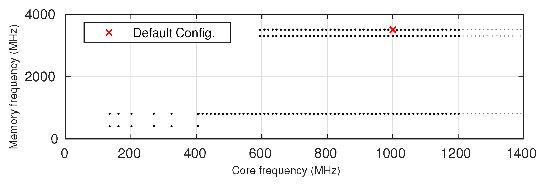
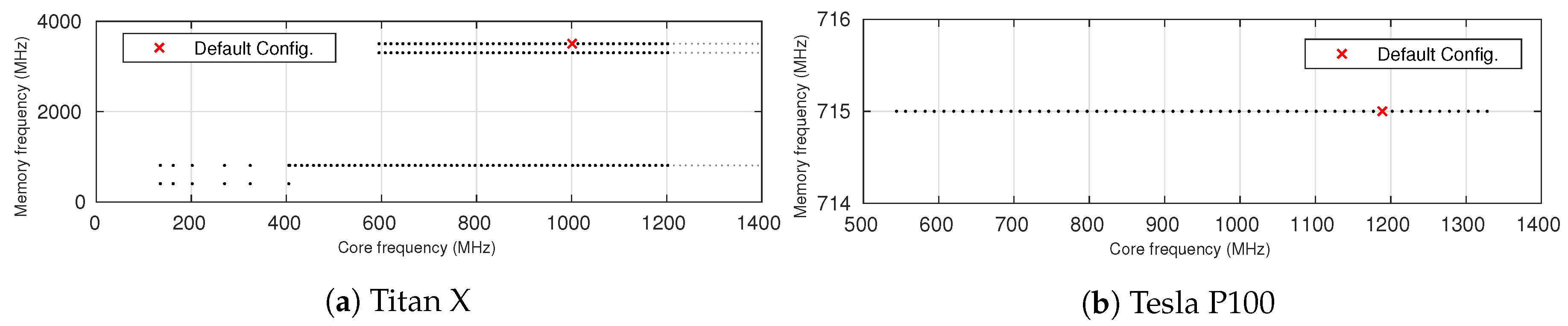
4.1. Frequency Domain and Test Setting
4.2. Imbalance of Available Frequency Configurations
5. Experimental Evaluation
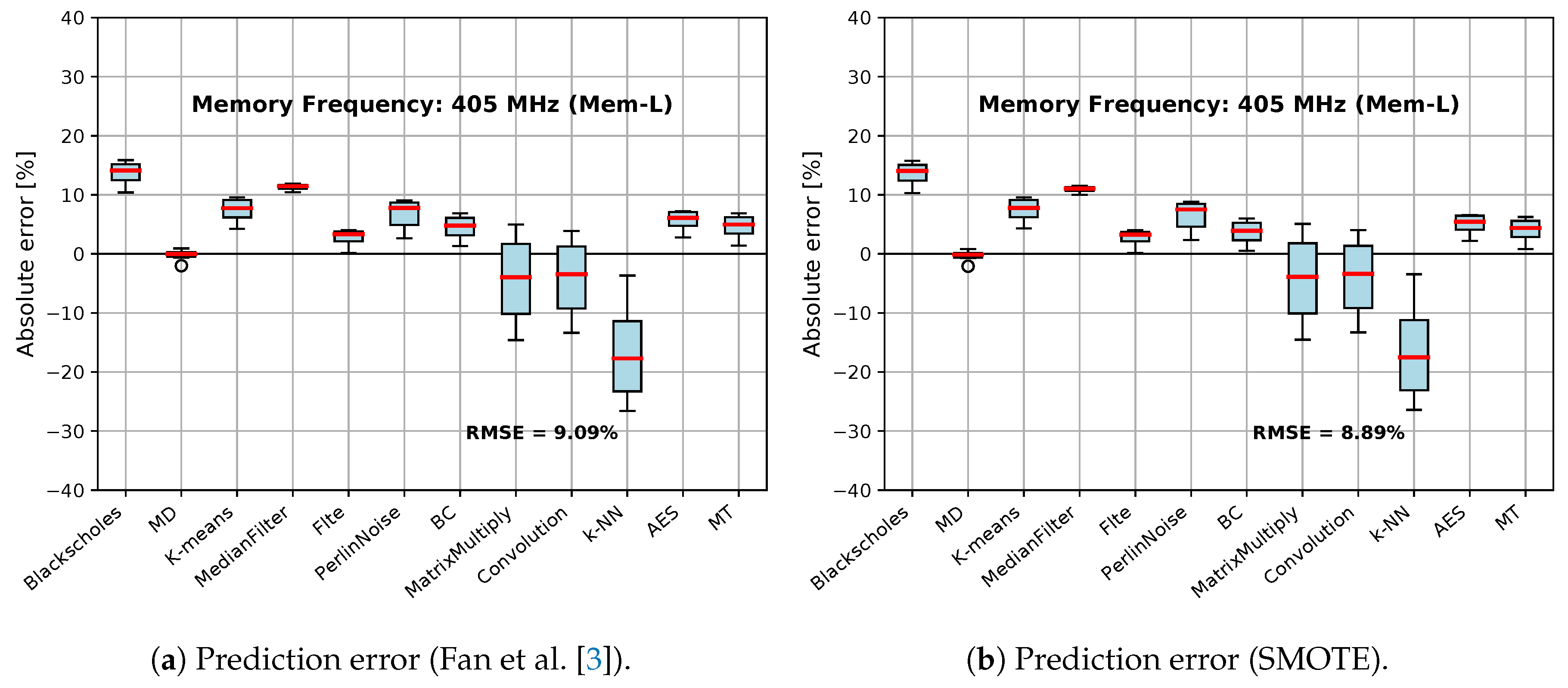
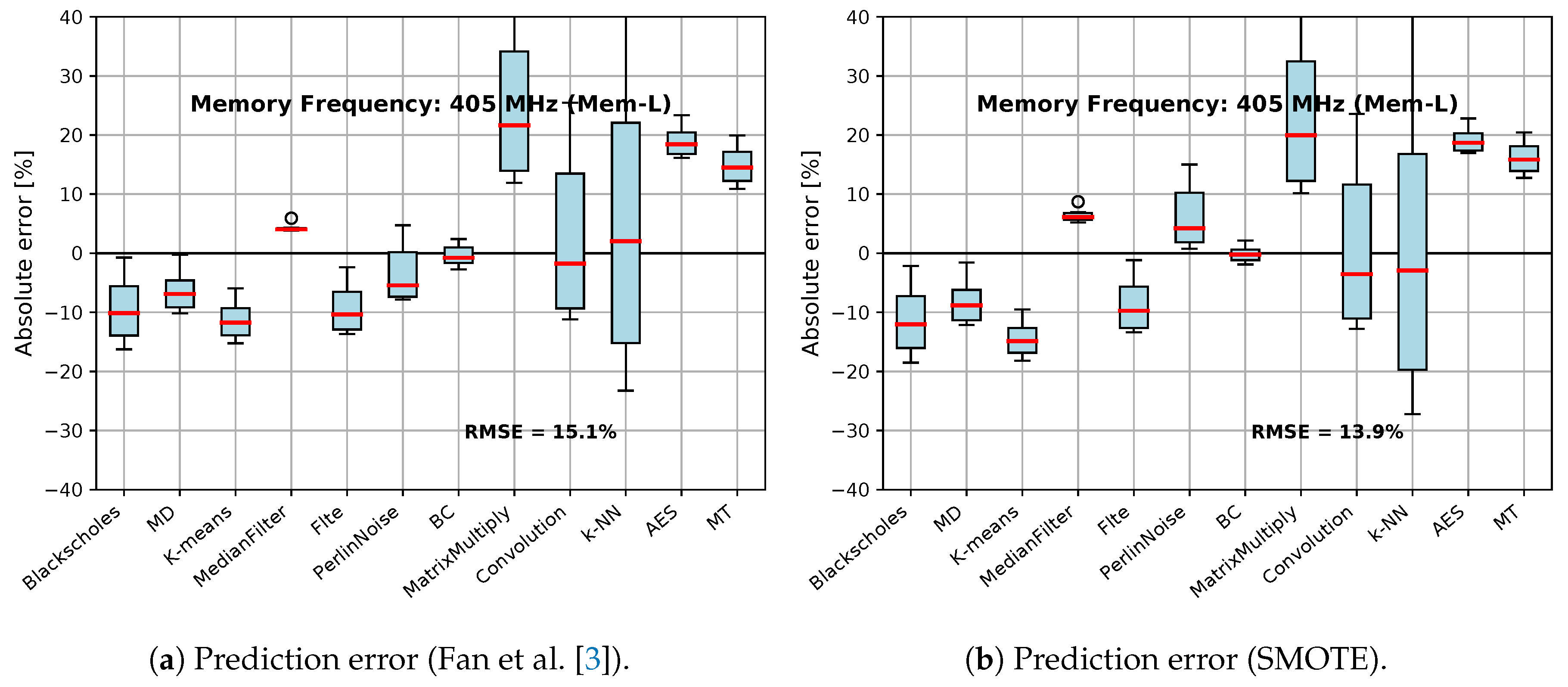
5.1. Experimental Evaluation of Oversampling
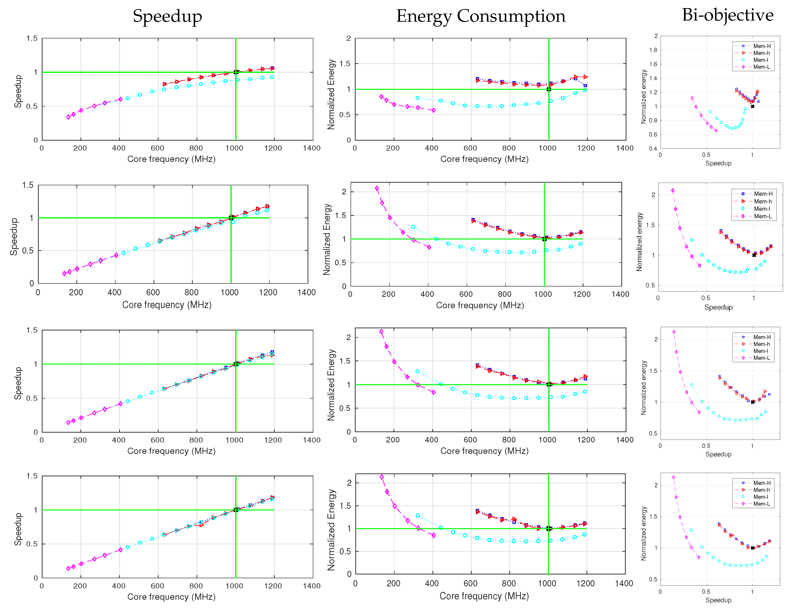
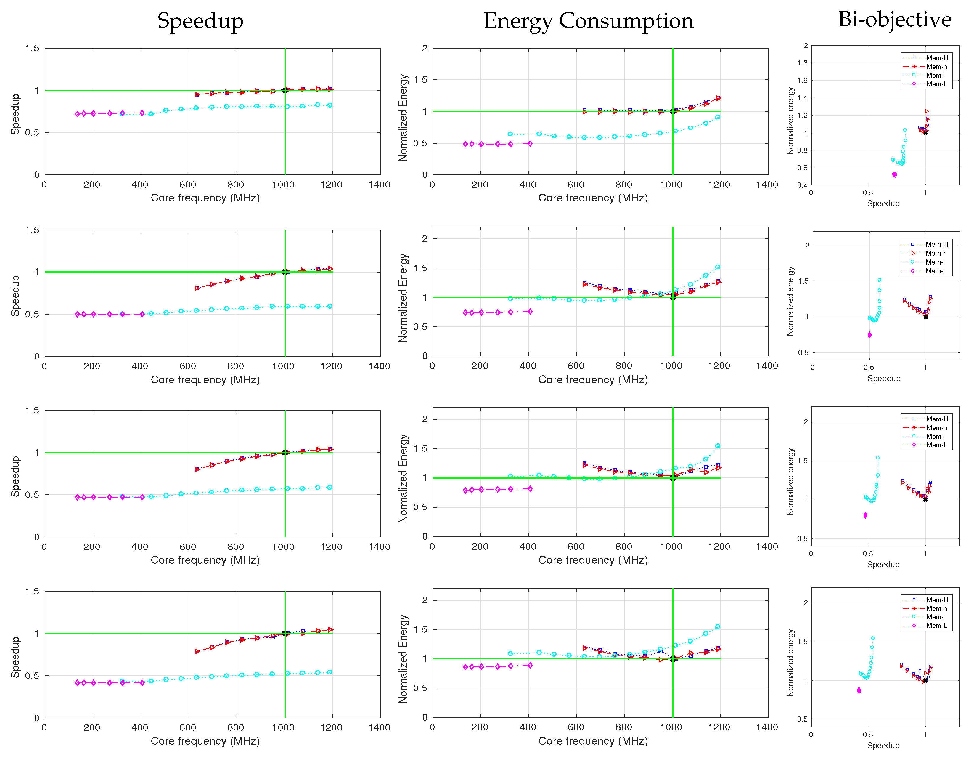
5.2. Application Characterization Analysis
5.3. Input-Size Analysis
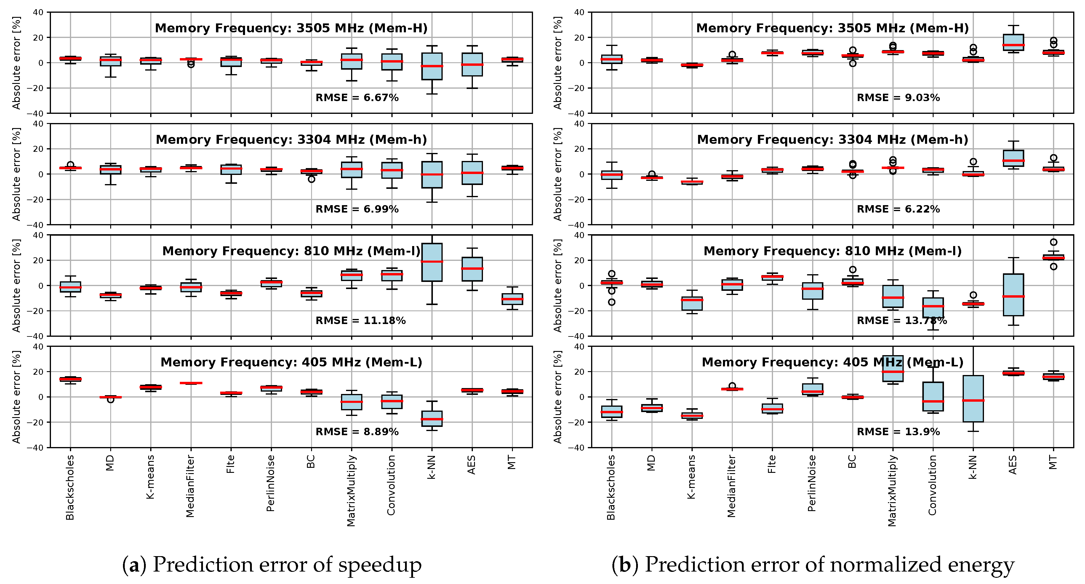
5.4. Accuracy of Speedup and Normalized Energy Predictions
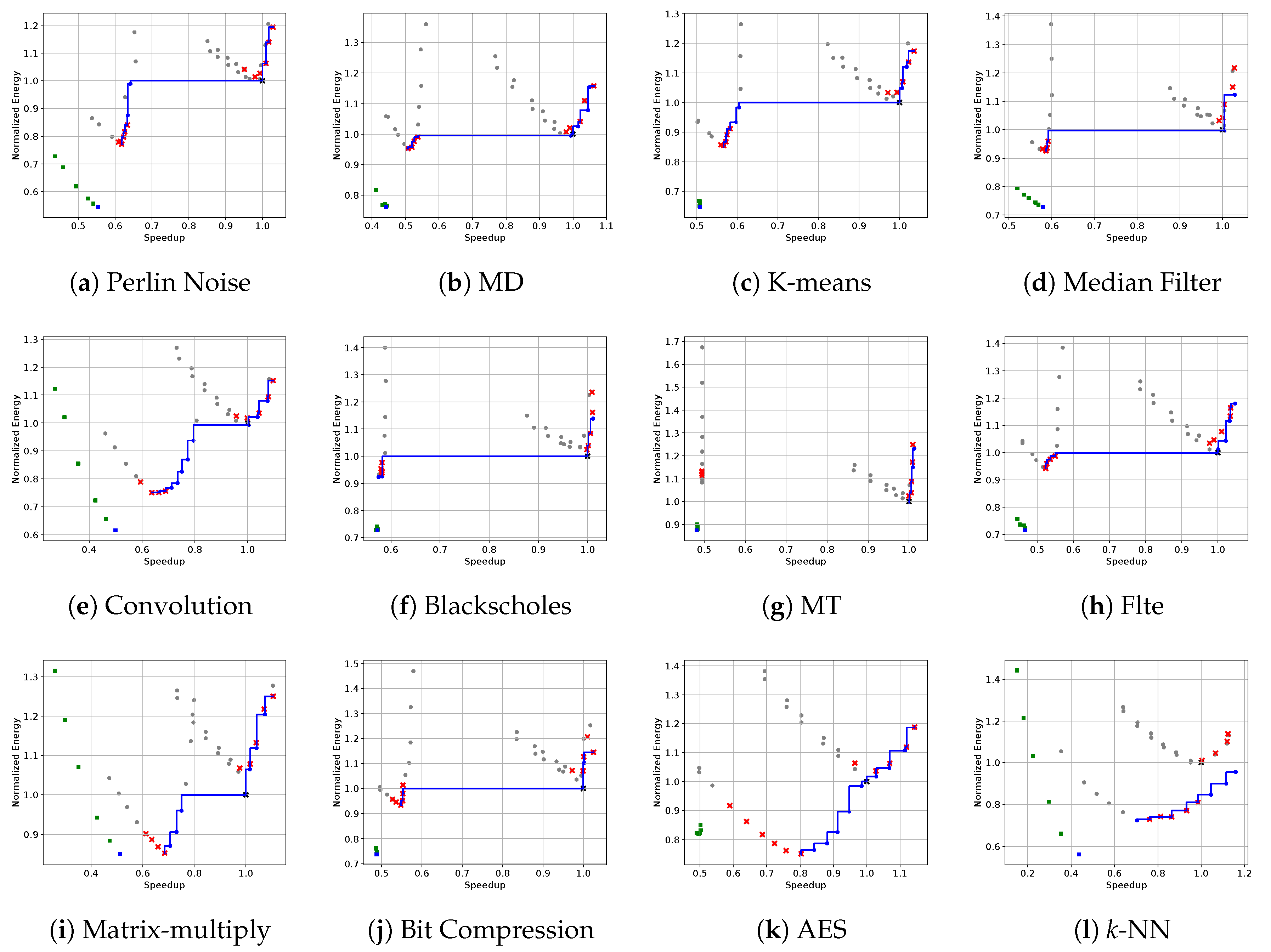
5.5. Accuracy of the Predicted Pareto Set
6. Conclusions
Author Contributions
Funding
Acknowledgments
Conflicts of Interest
References
- Intel. RAPL (Running Average Power Limit) Power Meter. Available online: https://01.org/rapl-power-meter (accessed on 24 April 2020).
- NVIDIA. NVIDIA Management Library (NVML). Available online: https://developer.nvidia.com/nvidia-management-library-nvml (accessed on 24 April 2020).
- Fan, K.; Cosenza, B.; Juurlink, B.H.H. Predictable GPUs Frequency Scaling for Energy and Performance. In Proceedings of the 48th International Conference on Parallel Processing, ICPP, Kyoto, Japan, 5–8 August 2019; pp. 52:1–52:10. [Google Scholar]
- Mei, X.; Yung, L.S.; Zhao, K.; Chu, X. A Measurement Study of GPU DVFS on Energy Conservation. In Proceedings of the Workshop on Power-Aware Computing and Systems, Berkleley, CA, USA, 3–6 November 2013; pp. 10:1–10:5. [Google Scholar]
- Calore, E.; Gabbana, A.; Schifano, S.F.; Tripiccione, R. Evaluation of DVFS techniques on modern HPC processors and accelerators for energy-aware applications. Concurr. Comput. Pract. Exp. 2017, 29, e4143. [Google Scholar] [CrossRef]
- Ge, R.; Vogt, R.; Majumder, J.; Alam, A.; Burtscher, M.; Zong, Z. Effects of Dynamic Voltage and Frequency Scaling on a K20 GPU. In Proceedings of the 42nd International Conference on Parallel Processing, ICPP, Lyon, France, 1–4 October 2013. [Google Scholar]
- Tiwari, A.; Laurenzano, M.; Peraza, J.; Carrington, L.; Snavely, A. Green Queue: Customized Large-Scale Clock Frequency Scaling. In Proceedings of the International Conference on Cloud and Green Computing, CGC, Xiangtan, China, 1–3 November 2012. [Google Scholar]
- Vysocky, O.; Beseda, M.; Ríha, L.; Zapletal, J.; Lysaght, M.; Kannan, V. MERIC and RADAR Generator: Tools for Energy Evaluation and Runtime Tuning of HPC Applications. In Proceedings of the High Performance Computing in Science and Engineering—Third International Conference, HPCSE, Karolinka, Czech Republic, 22–25 May 2017; Revised Selected Papers. pp. 144–159. [Google Scholar]
- Hamano, T.; Endo, T.; Matsuoka, S. Power-aware dynamic task scheduling for heterogeneous accelerated clusters. In Proceedings of the 23rd IEEE International Symposium on Parallel and Distributed Processing, IPDPS, Rome, Italy, 23–29 May 2009; pp. 1–8. [Google Scholar]
- Lopes, A.; Pratas, F.; Sousa, L.; Ilic, A. Exploring GPU performance, power and energy-efficiency bounds with Cache-aware Roofline Modeling. In Proceedings of the 2017 IEEE International Symposium on Performance Analysis of Systems and Software, ISPASS, Santa Rosa, CA, USA, 24–25 April 2017; pp. 259–268. [Google Scholar]
- Ma, K.; Li, X.; Chen, W.; Zhang, C.; Wang, X. GreenGPU: A Holistic Approach to Energy Efficiency in GPU-CPU Heterogeneous Architectures. In Proceedings of the 41st International Conference on Parallel Processing, ICPP, Pittsburgh, PA, USA, 10–13 September 2012; pp. 48–57. [Google Scholar]
- Song, S.; Lee, M.; Kim, J.; Seo, W.; Cho, Y.; Ryu, S. Energy-efficient scheduling for memory-intensive GPGPU workloads. In Proceedings of the Design, Automation & Test in Europe Conference & Exhibition, Dresden, Germany, 24–28 March 2014; pp. 1–6. [Google Scholar]
- Choi, J.; Vuduc, R.W. Analyzing the Energy Efficiency of the Fast Multipole Method Using a DVFS-Aware Energy Model. In Proceedings of the IEEE International Parallel and Distributed Processing Symposium Workshops, Chicago, IL, USA, 23–27 May 2016; pp. 79–88. [Google Scholar]
- Lee, J.H.; Nigania, N.; Kim, H.; Patel, K.; Kim, H. OpenCL Performance Evaluation on Modern Multicore CPUs. Sci. Program. 2015, 2015. [Google Scholar] [CrossRef]
- Shen, J.; Fang, J.; Sips, H.J.; Varbanescu, A.L. An application-centric evaluation of OpenCL on multi-core CPUs. Parallel Comput. 2013, 39, 834–850. [Google Scholar] [CrossRef]
- Harris, G.; Panangadan, A.V.; Prasanna, V.K. GPU-Accelerated Parameter Optimization for Classification Rule Learning. In Proceedings of the International Florida Artificial Intelligence Research Society Conference, FLAIRS, Key Largo, FL, USA, 16–18 May 2016; pp. 436–441. [Google Scholar]
- Pohl, A.; Cosenza, B.; Juurlink, B.H.H. Portable Cost Modeling for Auto-Vectorizers. In Proceedings of the 27th IEEE International Symposium on Modeling, Analysis, and Simulation of Computer and Telecommunication Systems, MASCOTS 2019, Rennes, France, 21–25 October 2019; pp. 359–369. [Google Scholar]
- Panneerselvam, S.; Swift, M.M. Rinnegan: Efficient Resource Use in Heterogeneous Architectures. In Proceedings of the 2016 International Conference on Parallel Architectures and Compilation, PACT, Haifa, Israel, 11–15 September 2016. [Google Scholar]
- Wang, Q.; Chu, X. GPGPU Performance Estimation with Core and Memory Frequency Scaling. In Proceedings of the 24th IEEE International Conference on Parallel and Distributed Systems, ICPADS 2018, Singapore, 11–13 December 2018; pp. 417–424. [Google Scholar] [CrossRef]
- Kofler, K.; Grasso, I.; Cosenza, B.; Fahringer, T. An automatic input-sensitive approach for heterogeneous task partitioning. In Proceedings of the International Conference on Supercomputing, ICS’13, Eugene, OR, USA, 10–14 June 2013; pp. 149–160. [Google Scholar]
- Ge, R.; Feng, X.; Cameron, K.W. Modeling and evaluating energy-performance efficiency of parallel processing on multicore based power aware systems. In Proceedings of the 23rd IEEE International Symposium on Parallel and Distributed Processing, IPDPS, Rome, Italy, 25–29 May 2009; pp. 1–8. [Google Scholar]
- Bhattacharyya, A.; Kwasniewski, G.; Hoefler, T. Using Compiler Techniques to Improve Automatic Performance Modeling. In Proceedings of the International Conference on Parallel Architecture and Compilation, San Francisco, CA, USA, 18–21 October 2015. [Google Scholar]
- De Mesmay, F.; Voronenko, Y.; Püschel, M. Offline library adaptation using automatically generated heuristics. In Proceedings of the 24th IEEE International Symposium on Parallel and Distributed Processing, IPDPS, Atlanta, GA, USA, 19–23 April 2010. [Google Scholar]
- Zuluaga, M.; Krause, A.; Püschel, M. e-PAL: An Active Learning Approach to the Multi-Objective Optimization Problem. J. Mach. Learn. Res. 2016, 17, 104:1–104:32. [Google Scholar]
- Grewe, D.; O’Boyle, M.F.P. A Static Task Partitioning Approach for Heterogeneous Systems Using OpenCL. In Proceedings of the 20th International Conference on Compiler Construction, CC, Saarbrücken, Germany, 26 March–3 April 2011; pp. 286–305. [Google Scholar]
- Den Steen, S.V.; Eyerman, S.; Pestel, S.D.; Mechri, M.; Carlson, T.E.; Black-Schaffer, D.; Hagersten, E.; Eeckhout, L. Analytical Processor Performance and Power Modeling Using Micro-Architecture Independent Characteristics. IEEE Trans. Comput. 2016, 65, 3537–3551. [Google Scholar] [CrossRef]
- Abe, Y.; Sasaki, H.; Kato, S.; Inoue, K.; Edahiro, M.; Peres, M. Power and Performance Characterization and Modeling of GPU-Accelerated Systems. In Proceedings of the IEEE 28th International Parallel and Distributed Processing Symposium, Phoenix, AZ, USA, 19–23 May 2014; pp. 113–122. [Google Scholar]
- Guerreiro, J.; Ilic, A.; Roma, N.; Tomás, P. GPU Static Modeling using PTX and Deep Structured Learning. IEEE Access 2019, 7, 159150–159161. [Google Scholar] [CrossRef]
- Guerreiro, J.; Ilic, A.; Roma, N.; Tomas, P. GPGPU Power Modelling for Multi-Domain Voltage-Frequency Scaling. In Proceedings of the 24th IEEE International Symposium on High-Performance Computing Architecture, HPCA, Vienna, Austria, 24–28 February 2018. [Google Scholar]
- Wu, G.Y.; Greathouse, J.L.; Lyashevsky, A.; Jayasena, N.; Chiou, D. GPGPU performance and power estimation using machine learning. In Proceedings of the 21st IEEE International Symposium on High Performance Computer Architecture, HPCA 2015, Burlingame, CA, USA, 2 October 2015; pp. 564–576. [Google Scholar]
- Isci, C.; Martonosi, M. Runtime Power Monitoring in High-End Processors: Methodology and Empirical Data. In Proceedings of the 36th Annual IEEE/ACM International Symposium on Microarchitecture (MICRO 36), San Diego, CA, USA, 5 December 2003. [Google Scholar]
- Cummins, C.; Petoumenos, P.; Wang, Z.; Leather, H. Synthesizing benchmarks for predictive modeling. In Proceedings of the International Symposium on Code Generation and Optimization, CGO, Austin, TX, USA, 4–8 February 2017; pp. 86–99. [Google Scholar]
- Cosenza, B.; Durillo, J.J.; Ermon, S.; Juurlink, B.H.H. Autotuning Stencil Computations with Structural Ordinal Regression Learning. In Proceedings of the IEEE International Parallel and Distributed Processing Symposium, IPDPS, Orlando, FL, USA, 29 May–2 June 2017; pp. 287–296. [Google Scholar]
- Smola, A.J.; Schölkopf, B. A tutorial on support vector regression. Stat. Comput. 2004, 14, 199–222. [Google Scholar] [CrossRef]
- Li, B.; Li, J.; Tang, K.; Yao, X. Many-Objective Evolutionary Algorithms: A Survey. ACM Comput. Surv. 2015, 48, 13:1–13:35. [Google Scholar] [CrossRef]
- Lemaître, G.; Nogueira, F.; Aridas, C.K. Imbalanced-learn: A Python Toolbox to Tackle the Curse of Imbalanced Datasets in Machine Learning. J. Mach. Learn. Res. 2017, 18, 1–5. [Google Scholar]
- Zitzler, E.; Thiele, L.; Laumanns, M.; Fonseca, C.M.; da Fonseca, V.G. Performance Assessment of Multiobjective Optimizers: An Analysis and Review. Trans. Evol. Comp. 2003, 7, 117–132. [Google Scholar] [CrossRef]
- Zitzler, E. Evolutionary Algorithms for Multiobjective Optimization: Methods and Applications. Ph.D. Thesis, University of Zurich, Zürich, Switzerland, 1999. [Google Scholar]


| Paper | Static | Pareto-Optimal | Frequency Scaling | Machine Learning |
|---|---|---|---|---|
| Grewe et al. [25] | ✓ | × | × | ✓ |
| Steen et al. [26] | × | ✓ | × | × |
| Abe et al. [27] | × | × | ✓ | × |
| Guerreiro et al. [29] | × | × | ✓ | ✓ |
| Wu et al. [30] | × | × | ✓ | ✓ |
| Our work | ✓ | ✓ | ✓ | ✓ |
| Benchmark | #Points | Extrema Point Distance | |||
|---|---|---|---|---|---|
| Max Speedup | Min Energy | ||||
| PerlinNoise | 0.0059 | 12 | 10 | (0.0, 0.0) | (0.009, 0.008) |
| MD | 0.0075 | 9 | 11 | (0.0, 0.0) | (0.0, 0.0) |
| K-means | 0.0155 | 10 | 12 | (0.0, 0.0) | (0.007, 0.003) |
| MedianFilter | 0.0162 | 11 | 6 | (0.001, 0.094) | (0.008, 0.006) |
| Convolution | 0.0197 | 10 | 14 | (0.0, 0.0) | (0.042, 0.038) |
| Blackscholes | 0.0208 | 9 | 7 | (0.002, 0.097) | (0.007, 0.016) |
| MT | 0.0272 | 10 | 6 | (0.003, 0.018) | (0.505, 0.114) |
| Flte | 0.0279 | 9 | 11 | (0.012, 0.016) | (0.0, 0.0) |
| MatrixMultiply | 0.0286 | 9 | 10 | (0.0, 0.0) | (0.073, 0.050) |
| BitCompression | 0.0316 | 11 | 6 | (0.0, 0.0) | (0.020, 0.023) |
| AES | 0.0362 | 11 | 14 | (0.0, 0.0) | (0.214, 0.165) |
| k-NN | 0.0660 | 9 | 8 | (0.036, 0.183) | (0.057, 0.004) |
© 2020 by the authors. Licensee MDPI, Basel, Switzerland. This article is an open access article distributed under the terms and conditions of the Creative Commons Attribution (CC BY) license (http://creativecommons.org/licenses/by/4.0/).
Share and Cite
Fan, K.; Cosenza, B.; Juurlink, B. Accurate Energy and Performance Prediction for Frequency-Scaled GPU Kernels. Computation 2020, 8, 37. https://doi.org/10.3390/computation8020037
Fan K, Cosenza B, Juurlink B. Accurate Energy and Performance Prediction for Frequency-Scaled GPU Kernels. Computation. 2020; 8(2):37. https://doi.org/10.3390/computation8020037
Chicago/Turabian StyleFan, Kaijie, Biagio Cosenza, and Ben Juurlink. 2020. "Accurate Energy and Performance Prediction for Frequency-Scaled GPU Kernels" Computation 8, no. 2: 37. https://doi.org/10.3390/computation8020037
APA StyleFan, K., Cosenza, B., & Juurlink, B. (2020). Accurate Energy and Performance Prediction for Frequency-Scaled GPU Kernels. Computation, 8(2), 37. https://doi.org/10.3390/computation8020037