Abstract
The thermo-structural design of the wing leading edge of hypersonic vehicles is a very challenging task as high gradients in thermal field, and hence high thermal stresses, are expected. Indeed, when employing passive hot structures based thermal protection systems, very high temperatures (e.g., 1400 °C) are expected on the external surface of the wing leading edge, while the internal structural components are required to not exceed a few hundred degrees Celsius (e.g., 400 °C) at the interface with the internal cold structure. Hence, ceramic matrix composites (CMC) are usually adopted for the manufacturing of the external surface of the wing leading edge since they are characterized by good mechanical properties at very high temperatures (up to 1900 °C) together with an excellent thermal shock resistance. Furthermore, the orthotropic behavior of these materials together with the possibility to tailor their lamination sequence to minimize the heat transferred to internal components, make them very attractive for hot structure based thermal protection systems applications. However, the numerical predictions of the thermo-mechanical behavior of such materials, taking into account the influence of each ply (whose thickness generally ranges between 0.2 and 0.3 mm), can be very expensive from a computational point of view. To overcome this limitation, usually, sub-models are adopted, able to focus on specific and critical areas of the structure where very detailed thermo-mechanical analyses can be performed without significantly affecting the computational efficiency of the global model. In the present work, sub-modeling numerical approaches have been adopted for the analysis of the thermo-mechanical behavior of a ceramic matrix composite wing leading edge of a hypersonic vehicle. The main aim is to investigate the feasibility, in terms of computational efficiency and accuracy of results, in using sub-models for dimensioning complex ceramic matrix components. Hence, a comprehensive study on the size of sub-models and on the choice of their boundaries has been carried out in order to assess the advantages and the limitations in approximating the thermo-mechanical behavior of the investigated global ceramic matrix composite component.
1. Introduction
The present work reports the follow-on research activity of a previous research work on the thermo-structural design of a ceramic matrix composite wing leading edge (WLE) of a re-entry vehicle [1]. Actually, in [1], the main aim was to minimize the thermal stresses occurring at the interfaces between the external hot structure and the internal cold structure by introducing new materials and new design solutions, in order to improve the design solutions described in [2] where ultra high temperature ceramics (UHTC) were employed. The results obtained in [1], in terms of weight savings and structural reliability, were considered very promising even if a simplified numerical model, based on an equivalent orthotropic material model, was adopted to simulate the skin of the WLE. Actually, with this material model, no information on the thermomechanical behaviour of each ply and its potential failure was available, leading to a very conservative design not fully exploiting the potential benefits of ceramic matrix composites.
Indeed, layered solid elements should have been adopted for a correct evaluation of the stress distribution and failure onset in each ply, but with a relevant decrease of the computational efficiency of the numerical analyses due to the increase of the number of elements and of the complexity of the element formulation.
The issue related to the reduction of computational efficiency when simulating the thermo-mechanical behaviour of complex ceramic matrix composite structures can be handled with the adoption of dedicated numerical approaches, such as global/local sub-modeling, able to provide detailed outputs only in specific critical locations of the component without significantly affecting the computational effectiveness related to the global model. Several works on the implementation of global/local and sub-modeling techniques in complex global models can be found in the literature [3,4,5,6,7,8,9,10]. Moller and Sundlo demonstrated the utility of the sub-modeling approach, to obtain accurate numerical results without significantly affecting the computational cost [11]. Indeed, they proved that the choice of solid elements and fine discretization in local models is, in many situations, mandatory to provide a realistic representation of the geometry and of the stress distribution, since such a representation cannot be provided by using shell elements and a coarser discretization. Ferraiuolo et al. showed that sub-modeling techniques are able to provide similar results, in terms of accuracy, if compared to global/local approaches, but with a considerable saving in terms of computational time [12]. Franzini applied the sub-modeling technique to study the structural behavior in specific locations of a plate subjected to plastic strains [13]. Actually, he implemented a two-way approach, according to which the results of the local model, on its boundary, are employed to correct the global model displacements iteratively as new boundary conditions for the local model. The loop stops when the variation in applied displacements at the boundaries falls within a specific tolerance range [14,15]. This approach seems to be particularly suited for thermo-mechanical applications, where nonlinear geometrical and material phenomena are accounted only in the local model. Shell-to-solid sub-modeling techniques have been investigated by Marenic et al. in order to obtain more realistic crack tip stress fields in linear elastic and non-linear elasto-plastic fracture mechanics applications [16].
In the present paper, the authors aim to demonstrate that sub-modeling techniques can represent a very valuable solution for the design of a complex component subjected to very high thermo-mechanical loads, such as the ceramic matrix composite wing leading edge of a re-entry vehicle.
Figure 1 and Figure 2 show the configuration resulting from the design process described in [1] that will be used at test bench in the present paper. Indeed, for this specific component, the need for detailed thermo-mechanical analyses is accompanied by the need for a detailed representation, at layer level, of the complex structure of ceramic matrix composite materials, leading to unfeasible computational costs.
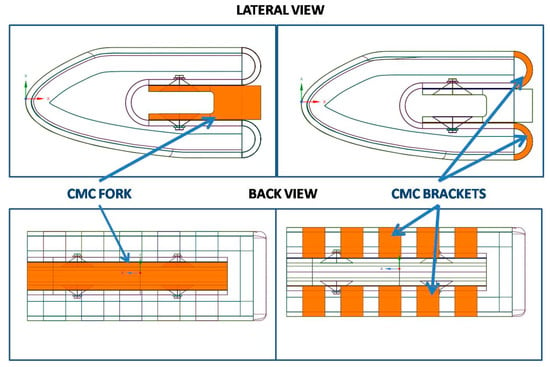
Figure 1.
Test Article Configuration—view 1.
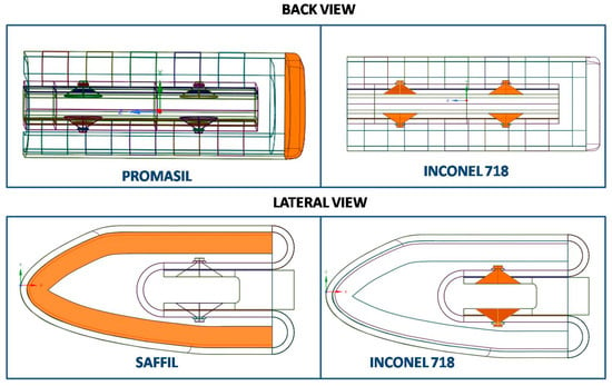
Figure 2.
Test Article Configuration—view 2.
In order to prove the feasibility of sub-modeling approach for the investigated component, a first set of trade off analyses has been performed to investigate the effects of the element formulation (shell or solid elements) adopted in the global coarse model, providing the boundary conditions for the local model, on the accuracy of results in the local solid model. Then, a further trade-off study has been performed by varying the size and the position of the local models, in order to assess the influence of these variations on the accuracy of the results and to identify general guidelines in the choice of local models.
2. Sub-Modeling
Sub-modeling is a finite element-based technique usually adopted to generate refined local models at specific locations in complex coarse global models. The idea of sub-modeling is a consequence of the De Saint-Venant’s Principle [17,18], which states that statically equivalent loading conditions, even if different, produce equivalent stress fields at a significant distance from the application location. Two distinct techniques can be adopted to exchange data form a global to a local model:
- node-based sub-modeling;
- surface-based sub-modeling.
The former approach uses interpolated temperature or displacement results from the global model as an input for the local model boundary nodes. The latter technique transfers the stress field computed at the global model level to the local model integration points. In the present paper, a node-based sub-modeling technique has been considered since, as demonstrated by Cormier [4], errors due to the discretization can be more effectively handled when displacements are used as input variables for the local models.
Two distinct solid local models have been considered in the frame of the investigations presented in this paper:
- Local Model 1: The temperature/displacements boundary conditions are taken from a global coarse shell model;
- Local Model 2: The temperature/displacements boundary conditions are taken from a global coarse solid model.
Clearly, the global coarse shell model is expected to be more computationally effective if compared to the corresponding solid model. Hence, the Local Model 2 is adopted later on to demonstrate the effectiveness of the Local Model 1 in terms of accuracy of results and computational efficiency with respect the full solid model.
Figure 3 shows the desired thermo-mechanical design loop with sub-modeling. First of all, the thermo-mechanical numerical analysis on the global coarse shell model is carried out, and boundary conditions (temperatures for the thermal analysis and displacements for the structural analysis) are assigned to the boundaries of the local model. Then, thermo-mechanical analyses are performed on the local refined model and Failure indexes at ply level are identified. If no failure is detected, no additional loop is needed, otherwise a change in design parameters (thickness, lamination sequence, or material system) followed by a new thermo-mechanical numerical analysis on the global coarse shell model is carried out to restart the design/dimensioning loop.
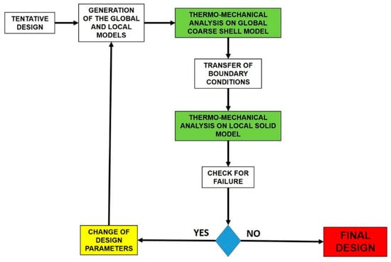
Figure 3.
Thermo-structural design loop.
As already remarked, a ceramic matrix composite WLE of a re-entry vehicle is the structure investigated in the frame of this paper. More specifically, a small portion of the wing leading edge has been considered of interest for verifying the capability of the presented sub-modeling approach to predict the thermo-mechanical behavior depending on the choice of design parameters such as thickness, lamination sequence and material systems.
In Figure 4 three Local models, named A, B, and C, with different sizes in the spanwise direction have been chosen with the aim to understand how the size of the model affects the themo-structural solution in the area of interest. The lengths of the Local models A, B, and C in the spanwise direction are respectively 20%, 30%, and 40% of the wingspan length.
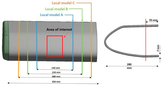
Figure 4.
Location and size of Local Models.
The majority of the components of the examined WLE are made of C/SiC (the external skin, the brackets connecting the external skin to the internal structure, the internal structure, and the support structure that must be connected to the model support system of the test facility), the fasteners connecting the internal structure to the support structure are made of Inconel 718. Moreover, Saffil is employed to protect the internal structure from internal radiation and Promasil is adopted to protect the internal structure from lateral external high heat fluxes.
It should be underlined that the aim of this paper is not the redesign of the component, but rather to demonstrate the advantages of the adoption of sub-modeling techniques to accurately and effectively predict the thermo-mechanical behavior of complex ceramic matrix composite components. As a matter of fact, the presented sub-modeling approach could be easily employed in the future to redesign and/or optimize the skin of the WLE presented in [1]. According to Figure 4, the size of the local model has been varied, in the frame of a preliminary trade-off study, to investigate the influence of the distance of the boundaries of the local model from the area of interest, on the accuracy of results.
3. Mathematical Model
3.1. Heat Conduction Modeling
The equations considered to solve heat conduction problems with radiation boundary conditions are presented hereafter [19]:
where:
- a is the thermal diffusivity;
- θ is the time;
- n is the direction normal to the external surface;
- Ts is the external surface temperature of the skin;
- σst is the Stefan-Boltzmann constant;
- αs is the surface absorptivity;
- qr is the incident radiation heat flux.
Temperature and heat flux continuity conditions are applied at the interfaces between different components.
3.2. Linear Elastic Modeling
The elastic equilibrium Equation is guaranteed by the following partial differential Equation [20,21,22,23]:
with σij representing the Cauchy stress tensor, and Xi representing the body force per unit volume. Compatibility Equations and Constitutive laws must be considered in order to find the deformed shapes and the stress fields.
4. Thermo-mechanical FEM Model Description
The ANSYS FEM (Finite Element Method) code [24] has been used to perform the thermo-mechanical analyses presented in this paper. As mentioned above, three different kinds of finite element models have been built:
- Global coarse model with shell elements for the skin profile;
- Global coarse model with solid elements for the skin profile;
- Local Solid model.
The global coarse models do not take into account the lamination sequence since they adopt an orthotropic equivalent material formulation for the ceramic matrix composite sub-components. The local solid model employs solid layered thermal/structural elements (SOLID90 for the thermal analyses and SOLID186 for the structural analyses) with mid-side nodes. The mapping algorithm, chosen to apply the boundary conditions (temperature or displacement) to the local model, is the shape function mapping algorithm which interpolates the displacement field coming from the global model using the shape functions of the elements considered in the local model. In this context, quadratic shape functions have been considered since the chosen element type (SOLID186) is characterized by the presence of midside nodes. The only parameter that should be provided to the finite element code is the normal distance, which represents the maximal distance that can be accepted in normal direction. In our case, the normal distance between the nodes of the global and local models is very short.
Table 1 summarizes the numerical analyses presented in this paper.

Table 1.
Overview the finite element analyses performed.
As can be seen in Table 1, a first numerical analysis on the full solid model (analysis 1) has been performed followed by analysis 2 and 3, respectively, on the global coarse solid and shell models. Finally, Analysis 4 and 5 have been performed on the local model, respectively, with boundary conditions taken from the global coarse shell and solid model. In Table 1, the trade-off analyses on the local model to investigate the influence of local model size on the accuracy of results have not been included.
4.1. Thermal and Structural Boundary Conditions
The aerodynamic heating maximum value encountered during the re-entry mission for the stagnation point is 400 kW/m2 and is reached after 1200 s. The entire re-entry trajectory lasts 3700 s [1].
Internal radiation boundary conditions have been set adopting a value for the emissivity of 0.8, while the external radiation emissivity is set to 0.9. Figure 5 shows that clamped structural boundary conditions have been applied to simulate the presence of the bolts connecting the Test Article to the Model Support System of the test facility in order to simulate the test in the plasma wind tunnel PWT (at the Italian Aerospace Research Centre facility) to be performed in a subsequent phase of the research programme.
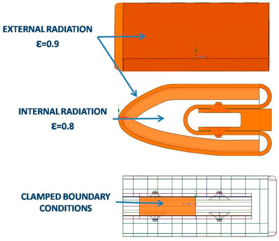
Figure 5.
Thermal and structural boundary conditions.
4.2. Thermo-Structural Elements and Material Properties
Shell elements with mid-side nodes have been used to model the wing leading edge in the global coarse shell model, while solid brick elements have been considered for the local models and for the global coarse solid model. The element type chosen for the thermal global shell analysis is “shell132” which is a three-dimensional layered quadratic shell element that takes into account in-plane and through-thickness thermal conductivity. The corresponding structural shell element, shell281, is also quadratic with six degrees of freedom at each node. A mesh convergence study has been conducted to the global and local models. The resulting least element edge lengths are reported below:
- Global shell model: 4.7 mm
- Global solid model: 4 mm
- Local models A, B and C: 0.3 mm
The different models for mesh convergence studies are shown in Figure 6.
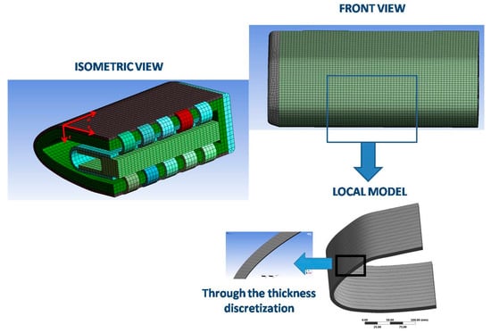
Figure 6.
Global coarse shell model—mesh.
In the following Table 2 and Table 3, the thermal and mechanical properties for all the materials systems involved in the computations are reported. C/SiC thermal and mechanical properties are referred to as “x”, “y”, and “z” directions depicted in Figure 6.

Table 2.
Thermo-mechanical properties at T = 700 °C.

Table 3.
C/SiC thermal and mechanical properties.
The quasi isotropic laminate stacking sequence [0/90/0/90/0/-45/45]2s with a ply thickness equal to 0.250 mm and an overall thickness equal to 7 mm, has been considered for all the C/SiC sub-components.
4.3. Failure Criteria
For the ceramic matrix composite sub-components, the maximum stress failure criterion has been adopted [25,26,27,28,29]. The failure index is evaluated according to the following equation taking into account the orthotropy of the material system:
where:
- , and represent the stress in the ply directions;
- are the tensile or compressive yield strengths in the x, y and z directions (tensile when and compressive when with );
- S, R, and Q are respectively the shear strengths in the (xy), (xz) and (yz) planes;
- are respectively the shear stresses in the (xy), (xz) and (yz) planes;
5. Results and Discussions
As mentioned in the previous section, two global coarse finite element models, a full model, and a local model have been built. Thermomechanical analyses on the global models and on the full refined model have been carried out. After a preliminary trade-off study on the influence of local model size on accuracy of results, two thermo-structural analyses with two different sets of boundary conditions have been performed on the local model: the first set is taken from the global coarse shell model, while the second one is taken from the global coarse solid model. Hereafter, the obtained results on global model and local model are introduced and discussed.
5.1. Global Coarse Shell Model
Figure 7 shows the temperature distribution on the global coarse shell model after 1200 s where maximum heat fluxes are expected. The maximum computed temperature is 1116 °C.
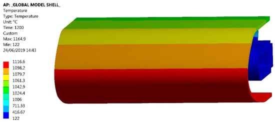
Figure 7.
Temperature contour plot at 1200 s—Global coarse shell model.
Figure 8 shows the magnitude of the displacements obtained by means of a static structural analysis considering as input the thermal loads reported in Figure 7. An amplification factor of seven has been used.
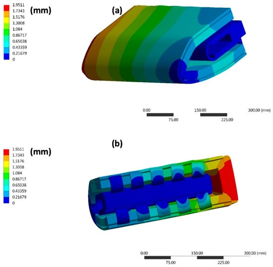
Figure 8.
Displacements (magnitude) at 1200 s - Global coarse shell model: (a) front view; (b) rear view—Amplification factor: 7.
5.2. Global Coarse Solid Model
Figure 9 shows the temperature distribution on the global coarse solid model after 1200 s where maximum heat fluxes are expected. The maximum computed temperature is almost 1100 °C. It can be easily noticed that the temperature distribution is very similar to the one found by adopting the global coarse shell model (there is only less than 20 °C temperature difference between the examined global models). Furthermore, since the skin is very thin and the maximum thermal gradients act in the skin direction, no significant temperature variations have been detected in the thickness direction for the skin.
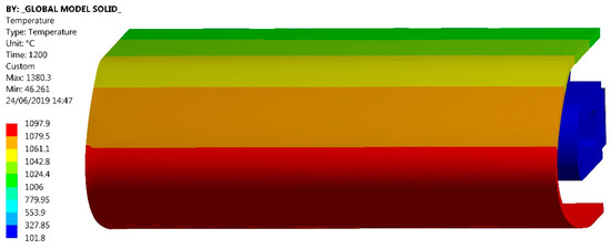
Figure 9.
Temperature contour plot at 1200 s -Global coarse solid model.
Figure 10 shows the magnitude of the displacements of the global solid model. Displacement values are very similar to those shown in Figure 8 for the global coarse shell model. The amplification factor adopted is seven.
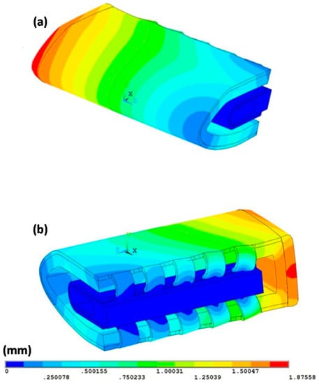
Figure 10.
Displacements (magnitude)—Global coarse solid model: (a) front view; (b) rear view. Amplification factor: 7.
The percentage difference between the maximum temperatures achieved in the global shell model and the global solid model is 1.7%. Very similar results are obtained when comparing the global shell model with the solid local models. With regard to the displacements, the percentage difference between the global shell model and the global solid model is 4%.
5.3. Local Models
Several analyses have been performed on the local models. First of all, a preliminary trade-off study has been performed varying the size of the model according to Figure 4. In Table 4, the failure indexes, used as control parameter to evaluate the influence of local model size, are summarized at ply level for each local model.

Table 4.
Failure indexes for 1–4 and 24–28 plies.
It is clear that the failure indexes achieved with the smallest local model (local model A) are strongly influenced by its boundaries that are very close to the area of interest. On the other hand, local models B and C, provide very similar results. Hence, the local model B has been chosen for the rest of the analyses because it seems undoubtedly the best choice being significantly smaller if compared to local model C.
A convergence analyses has been performed on the local model B in order to minimize the number of elements to be used to obtain an accurate solution. Table 5 summarizes the results of the convergence study where “SIZING 1” refers to a mesh with 25,000 elements, “SIZING 2” to a mesh with 50,000 elements and “SIZING 3” to a mesh with 70,000 elements. The least element edge length values for “sizing 1–3” are:

Table 5.
Mesh convergence analysis (Model B) results.
- 0.3 mm for “sizing 1”
- 0.2 mm for “sizing 2”
- 0.1 mm for “sizing 3”
According to the results of Table 5, the local model B with 25,000 elements has been adopted for the rest of the analyses presented in this Section.
In Figure 11 and Figure 12, the results of the thermal analyses on the local model B (of Figure 4) with temperature boundary conditions taken, respectively, from the global coarse shell and solid model, at 1200 s, are presented. As expected, the results are very similar. It is interesting to note that little differences between maximum temperature values were detected with respect to the global analyses where the lamination sequence has not been taken into account (1095 °C for the local solid model and 1116°C for the global coarse shell model).
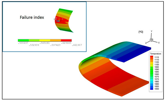
Figure 11.
Temperature contour plot at 1200 s—Local model B—BC taken from the global coarse shell model—Temperatures are expressed in °C.
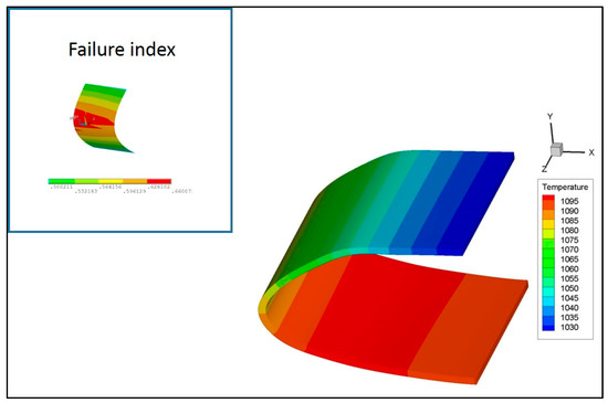
Figure 12.
Temperature contour plot at 1200 s—Local model B—BC taken from the global coarse solid model—Temperatures are expressed in °C.
Failure indexes obtained with the local models employing temperature and displacement boundary conditions coming from the global coarse shell and solid model are reported in Table 6. It is easy to notice that the results in terms of failure indexes are very similar.

Table 6.
Comparison between failure indexes from local models with BCs taken from global coarse shell and solid models.
Finally, the authors have investigated the influence of the local models size on the structural analyses results. Considerations obtained for the thermal analyses can be repeated showing that local model B and C are the best choices.
5.4. Full Model
Finally, a thermo-mechanical analysis on a full refined model has been carried out. The temperature distribution, evaluated by means of the thermal analysis, shows that the results of the local models, illustrated in the previous paragraphs, are very accurate (see Figure 13). The maximum temperature value at 1200 s in the area of interest is 1097 °C which is very close to the one predicted with the local models (1095 °C and 1115 °C).
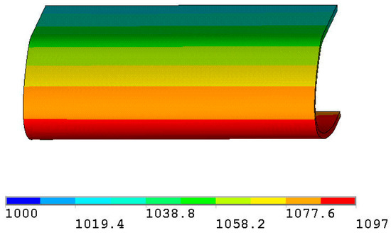
Figure 13.
Temperature contour plot at 1200 s - Full refined model.
However, the failure index values computed in the area of interest with the sub-models and with the full refined model are not as close to each other as the temperature values. Then, the boundary conditions have, definitively, a non-negligible impact on the results of the local models. Nevertheless, looking at the differences in failure indexes (0.61 for the full refined model and 0.66 for the local model B for the 90° oriented plies), adopting the local models in the design process seems to be still a very good option since a conservative result is achieved.
Finally, Figure 14, showing the maximum failure indexes obtained with the full refined model, points out that sub-models should be created for specific areas of the test article which appears to be critical. In fact, at the interface between the brackets connecting the external and the internal structure (see the grey areas in Figure 14) failure indexes exceed the unit value. More specifically, the connection of the brackets to the external surface do not cover the entire cross-sectional area of the wing leading edge. Then, the thermal resistance to the heat flux in the chord-wise direction increases, generating high thermal gradients. This kind of criticality was not accounted for in the previous design activity [1].
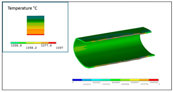
Figure 14.
Maximum failure indexes at 1200 s - Full model.
6. Summary and Conclusions
In the present paper, the advantages of adopting numerical sub-modeling approaches to design a test article representing the wing leading edge of a re-entry vehicle have been exploited.
The solution “global coarse shell models to local solid model”, according to which a global coarse shell model is adopted to provide boundary conditions for the local model, provides results very similar to the one obtained with the “global coarse solid models to local solid model” approach (a global coarse solid model is adopted to provide boundary conditions to a solid local model), in terms of both predicted temperature and structural failures.
Investigation on a full refined global model has also demonstrated that the results, in terms of failure indexes, obtained with the local models are conservative (8% higher than those obtained with the fully refined model). On the other hand, the temperature distribution along the profile of the WLE are almost the same between the local models and the full refined global model.
These outcomes are very interesting because they demonstrate that very fast global coarse shell models, associated to a local solid model, can provide a realistic overview of the thermo-mechanical behaviour of complex ceramic matrix composite components with a considerably lower computational effort if compared to fully refined global models. Hence, these sub-models could be easily included in a design loop trying to identify an optimized configuration of the WLE by changing design parameters. Finally, a trade-off analysis on differently sized local models has been also carried out to identify some useful guidelines for the choice of the best suited size and boundaries of the local models. As expected, the boundaries of the local models cannot be close to the area of interest to guarantee accurate predictions.
Furthermore, the results have demonstrated that the adoption of sub-modeling techniques allows to significantly improve the computational efficiency: in fact, the CPU time needed to perform global coarse and local refined analyses is four times smaller than the CPU time required to conduct one global refined analysis. Then, in a design loop process, such as that proposed in the present work, the length of design activities can be considerably reduced. Furthermore, the choice of global shell models makes the potential change of thickness very simple if compared to the fully refined model where a new CAD model should be generated.
Author Contributions
Conceptualization, M.F., C.P., A.S. and A.R.; Data curation, M.F., C.P., A.S. and A.R; Investigation, M.F., C.P., A.S. and A.R.; Writing—original draft, M.F., C.P., A.S. and A.R. All authors have read and agreed to the published version of the manuscript.
Funding
This research received no external funding.
Conflicts of Interest
The authors declare no conflict of interest.
References
- Ferraiuolo, M.; Scigliano, R.; Riccio, A.; Bottone, E.; Rennella, M. Thermo-structural design of a Ceramic Matrix Composite wing leading edge for a re-entry vehicle. Compos. Struct. 2019, 207, 264–272. [Google Scholar] [CrossRef]
- Fossati, F.A.; D’Aversa, E.; Marchetti, M.; Marino, G.; Testani, C. Enabling technologies for hot structures of next generation RLV’s—The ASA program summary. Int. Astronaut. Congr. 2010, 10, 8549–8553. [Google Scholar]
- Sracic, M.W.; Elke, W.J. Effect of boundary conditions on finite element submodeling. Conf. Proc. Soc. Exp. Mech. Ser. 2019, 1, 163–170. [Google Scholar]
- Cormier, N.G.; Smallwood, B.S.; Sinclair, G.B.; Meda, G. Aggressive submodelling of stress concentrations. Int. J. Numer. Methods Eng. 1999, 46, 889–909. [Google Scholar] [CrossRef]
- Gendre, L.; Allix, O.; Gosselet, P.; Comte, F. Non-intrusive and exact global/local techniques for structural problems with local plasticity. Comput. Mech. 2009, 44, 233–245. [Google Scholar] [CrossRef]
- Mao, K.M.; Sun, C.T. A refined global-local finite element analysis method. Int. J. Numer. Methods Eng. 1991, 32, 29–43. [Google Scholar] [CrossRef]
- Gosselet, P.; Blanchard, M.; Allix, O.; Guguin, G. Non-invasive global–local coupling as a Schwarz domain decomposition method: Acceleration and generalization. Adv. Model. Simul. Eng. Sci. 2018, 5, 4. [Google Scholar] [CrossRef]
- Duval, M.; Passieux, J.C.; Salaün, M.; Guinard, S. Local/global non-intrusive parallel coupling for large scale mechanical analysis. In Proceedings of the 11th World Congress on Computational Mechanics, WCCM 2014, Barcelona, Spain, 20–25 July 2014; pp. 1920–1931. [Google Scholar]
- Kilic, B.; Madenci, E.; Ambur, D.R. Global-local finite element analysis of bonded single-lap joints. Struct. Struct. Dyn. Mater. Conf. 2004, 1, 542–554. [Google Scholar]
- Sellitto, A.; Borrelli, R.; Caputo, F.; Riccio, A.; Scaramuzzino, F. Methodological Approaches for Kinematic Coupling of nonmatching Finite Element meshes. Procedia Eng. 2011, 10, 421–426. [Google Scholar] [CrossRef][Green Version]
- Moller, C.; Sundlo, O. Method for Merging Scales in Finite Element Analyses, Framework for Automated Global/Local Analyses. Master’s Thesis, Department of Applied Mechanics Chalmers University of Technology, Austin, TX, USA, 2017. [Google Scholar]
- Ferraiuolo, M.; Palumbo, C.; Sellitto, A.; Riccio, A. Global/Local Finite Element Analyses Supporting The Design Of A Ceramic Matrix Composite Wing Leading Edge Of A Re-Entry Vehicle. Mater. Today Proc. 2020. submitted. [Google Scholar] [CrossRef]
- Franzini, G. Modellazione Strutturale Multi-Livello Utilizzando un Codice FEM Commerciale; Politecnico Di Milano, Scuola di Ingegneria Industriale e dell’Informazione: Milan, Italy, 2016–2017. [Google Scholar]
- Whitcomb, J.D. Iterative global/local finite element analysis. Comput. Struct. 1991, 40, 1027–1031. [Google Scholar] [CrossRef]
- Whitcomb, J.D.; Woo, K. Application of iterative global/local finite-element analysis. Part 1: Linear analysis. Commun. Numer. Methods Eng. 1993, 9, 745–756. [Google Scholar] [CrossRef]
- Marenić, E.; Skozrit, I.; Tonković, Z. On the calculation of stress intensity factors and J-integrals using the submodeling technique. J. Press. Vessel Technol. Trans. Asme 2010, 132, 041203. [Google Scholar] [CrossRef]
- De Saint-Venant, A.J.C.B. Memoire Sur La Torsion Des Prismes. Mem. Divers. Savants. 1855, 14, 233–560. [Google Scholar]
- Von Mises, R. On Saint-Venant’s principle. Bull. Am. Math. Soc. 1945, 51, 555–562. [Google Scholar] [CrossRef]
- Ozisik, N. Heat Conduction; Wiley: New York, NY, USA, 1980. [Google Scholar]
- Hetnarski, R.; Eslami, M. Thermal Stresses: Advanced Theory and Applications; Springer: Dordrecht, The Netherlands, 2009; ISBN 978-1-4020-9246-6. [Google Scholar]
- Thornton, E. Thermal Structures for Aerospace Applications; AIAA: Reston, VA, USA, 1996. [Google Scholar]
- Boley, B.A.; Weiner, J.H. Theory of Thermal Stresses; Dover Publications: New York, NY, USA, 1960. [Google Scholar]
- Mahdavi, E.; Ghasemi, A.; Alashti, R.A. Elastic–plastic analysis of functionally graded rotating disks with variable thickness and temperature-dependent material properties under mechanical loading and unloading. Aerosp. Sci. Technol. 2016, 59, 57–68. [Google Scholar] [CrossRef]
- ANSYS® Academic Research, Release 16; ANSYS Inc.: Canonsburg, PA, USA, 2017.
- Tsai, S.W.; Wu, E.M. A General Theory of Strength for Anisotropic Materials. J. Compos. Mater. 1971, 5, 58–80. [Google Scholar] [CrossRef]
- Jones, R.M. Mechanics of Composite Materials, (Materials Science & Engineering Series), 2nd ed.; CRC Press: Philadelphia, PA, USA, 1999. [Google Scholar]
- Jun, L.; Guiqiong, J.; Bo, W.; Chengpeng, Y.; Gang, W. Damage characteristics and constitutive modeling of the 2D C/SiC composite: Part I—Experiment and analysis. Chin. J. Aeronaut. 2014, 27, 1586–1597. [Google Scholar]
- Li, J.; Jiao, G.; Wang, B.; Li, L.; Yang, C. Damage characteristics and constitutive modeling of the 2D C/SiC composite: Part II—Material model and numerical implementation. Chin. J. Aeronaut. 2015, 28, 314–326. [Google Scholar] [CrossRef]
- Shojaei, A.; Li, G.; Fish, J.; Tan, P.J. Multi-scale constitutive modeling of ceramic matrix composites by continuum damage mechanics. Int. J. Solids Struct. 2014, 51, 4068–4081. [Google Scholar] [CrossRef]
© 2020 by the authors. Licensee MDPI, Basel, Switzerland. This article is an open access article distributed under the terms and conditions of the Creative Commons Attribution (CC BY) license (http://creativecommons.org/licenses/by/4.0/).