1. Introduction
Wave run-up is the maximum vertical limit of wave upsurge which occurs on a beach or structure above the still water level. In the tsunami mitigation plan, a good estimation of wave run-up is needed to determine the evacuation area to protect people from the tsunami. Many researchers developed empirical formulas to predict the run-up for regular waves [
1,
2,
3]. Analytical formulation of wave run-up was also derived for different types of incident waves based on Carrier and Greenspan’s solution [
4,
5,
6]. Both empirical and analytical formulas are useful for practical application but they are generally limited to a simplified sloping structure. For more complex topography and general type of waves, the numerical approach is necessary to predict the wave run-up.
Several wave models can be used to approximate the wave run-up. Shallow water equations are often used in wave run-up models, especially in tsunami cases. The numerical scheme based on shallow water equations is good enough to simulate wave run-up for long waves [
7,
8]. However, for dispersive waves, i.e., solitary waves, this model failed to simulate the propagation with the correct speed. Thus, another model is needed in dispersive wave modelling.
There are two approaches to model the dispersive waves, i.e., Boussinesq-type and non-hydrostatic approaches. The Boussinesq-type model was constructed for irrotational and incompressible fluid flow without friction [
9,
10,
11]. Nevertheless, the difficulty in dealing with the Boussinesq model is due to the complexity of non-linearity and dispersion terms. An alternative model that involves non-linearity and dispersion is the depth integrated non-hydrostatic model which was firstly developed by [
12] to solve Euler equations with total pressure. Then, this total pressure was separated by [
13] and [
14] into hydrostatic and hydrodynamic pressure to improve the efficiency of the computational time.
Stelling and Zijlema (2003) [
15] in SWASH and Magdalena [
16] proposed an alternate depth-integrated formulation, which introduces non-hydrostatic pressure and vertical velocity terms in the non-linear shallow water equations (NSWE) to describe weakly dispersive waves. The paper presents some validations of the scheme by making a comparison between the numerical results and analytical solution, also with the experimental data. To obtain a good agreement with both analytical and experimental results, it is necessary to use two or more layers. Based on the scheme introduced by Stelling and Zijlema (2003), we propose a modification of two-layer non-hydrostatic approach.
Here, we study the performance of the modified two-layer scheme. It can handle wave frequency correctly including short waves up to
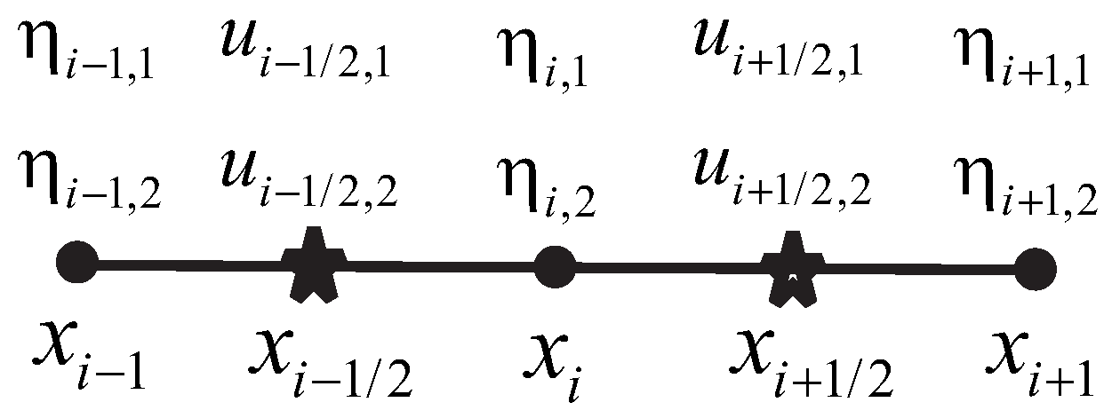
kd ≈ 6. For the application of two-layer fluid system, this scheme can simulate soliton propagation with undisturbed shape. Therefore, we can conclude that the modified two-layer scheme can balance the non-linearity and dispersion effects. This is the most important test case for non-linear and dispersive model. In this research, first, we construct a momentum conservative numerical scheme without considering the dispersion effect using a staggered finite volume method. This method, which was initially investigated by [
17] to solve differential equations, was further extended and implemented by many researchers [
15,
18,
19]. Working with a staggered finite volume gives us more advantages than working in a collocated grid because we do not end up with the Riemann problem that is relatively difficult to solve, as seen in the NHWAVE proposed by [
20]. Besides, this scheme could give accurate result for subcritical flow [
21] and relatively simple even for three-dimensional extent [
14,
22,
23]. Secondly, to derive the model with dispersion, we propose a non-hydrostatic approach that incorporates hydrodynamic pressure. By taking the hydrodynamic pressure into account, we consider inhomogeneity in vertical direction. This two-layer approach has a tridiagonal matrix for pressure, whereas the standard two-layer approach in SWASH by Stelling and Zijlema (2003) has a pentadiagonal matrix. Dealing with a tridiagonal matrix allows us to implement the Thomas algorithm, which is faster than a pentadiagonal matrix that needs to be solved using an iterative method. Thus, the computational cost of this two-layer approach is comparable with that of the one-layer approach [
24], but the performance is comparable with the two-layer approach as conducted in Stelling and Zijlema (2003). We can argue that this two-layer approach is efficient.
In this paper, we will see how wide the range of problems that can be covered by the numerical scheme is. A series of test cases will be conducted to validate and verify the two-layer non-hydrostatic numerical scheme. First, we will simulate the propagation of solitary waves over a flat bottom topography. Then, the topography will be extended to a sloping beach with and without a reef. The results will be compared to the data measured in laboratory experiments. Finally, the numerical scheme is implemented to simulate the 2004 Indian Ocean tsunami run-up on the west coast of Aceh, Indonesia.
2. The Two-Layer Non-Hydrostatic Model
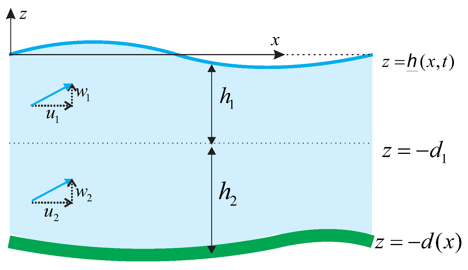
In this section, we explain briefly the derivation of the non-hydrostatic model using the two-layer approach to study wave run-up over a sloping beach. First, we consider our observation domain as a two-layer fluid system, upper and lower layer domain, that are indexed by subscript 1 and 2, respectively. The sketch of this problem is shown in
Figure 1. Here,
denotes the bottom topography, while
denotes the free surface elevation. The interface between the two layers is located at
. The water thickness for each layer is
for
. The horizontal and vertical velocity is denoted by
and
, respectively.
Our derivation based on the Euler equations model in terms of the velocity
read as
where
q is the essential term in this model that is our hydrodynamic pressure. Respectively, the kinematic free surface and bottom boundary conditions for the flow read as:
The subscripts
and
d denote the position where quantity evaluated. Based on the Euler equations above, we integrate Equations (1) and (2) from the bottom to the interface. By implementing the kinematic boundary condition (5) and Leibniz’s rule, we obtain
Similarly, for the upper layer, incorporating the kinematic boundary condition (
4) and Equation (
6) into the integration of Equations (
1) and (2) from the interface to the surface, we obtain
Under the assumption that
, then the momentum Equation (
8) becomes
In this non-hydrostatic approach, vertical homogeneities are adopted. The relations between vertical velocity and hydrodynamic pressure
q for the two layers come from the linearized momentum equation with the Keller-box scheme read as
The closure relations needed to calculate
and
come from the mass conservation for both layers as follows.
To eliminate the vertical velocity and the pressure at the bottom from the set of equations, first, Equation (
12) is multiplied by 2, then added to Equation (13):
From now on, we treat as a new variable.
Here, we assume the fluid density profile increases with depth only in the upper part of a fluid column. In the lower part, fluid density value is nearly constant, as commonly observed in nature. Therefore, the hydrodynamic pressure
q is assumed to be a constant function throughout the lower layer. In this two-layer formulation, we denote
, so that Equation (7) is simplified to
Finally, the full set of non-hydrostatic model using two-layer approach is
The system consists of five equations with five unknown variables , and . This gives us an advantage in the computation where we do not need to compute Equation (11) anymore.
3. Dispersion Relation
In this section, we derive the dispersion relation of our linearized two-layer non-hydrostatic model over a constant depth
where
and
. To derive the dispersion relation of the proposed model, first, we assume that the wave is a periodic wave with a small amplitude in the form of
Notation
denotes wave celerity, and
k is the wavenumber. Substituting Equations (
21)–(
25) into the linearized governing equations written as
we obtain the following dispersion relation,
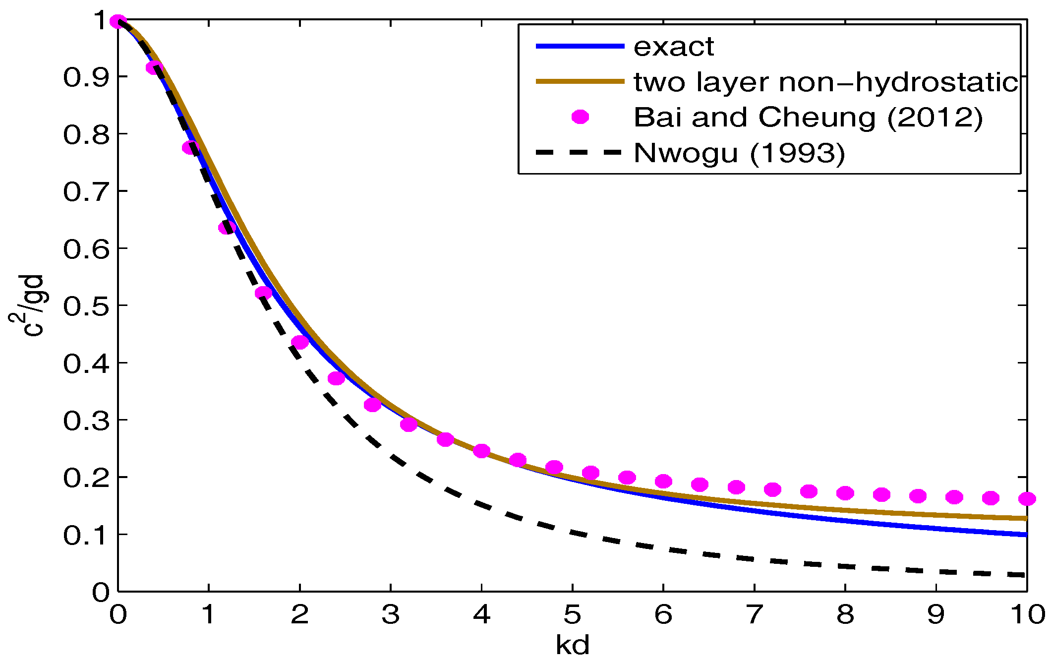
To check the accuracy of our dispersion relation, we compare it with the dispersion relation proposed by [
10] and [
25]. Nwogu [
10] obtained the dispersion relation of Boussinesq-type model written as
where
is a parameter that was adjusted to be equal to −1/3 in order to get the result closer to the exact dispersion relation. The linear dispersion relation of the hybrid system obtained by Bai and Cheung wrote as
where
is a free parameter.
For the comparison between the exact dispersion relation with the ones obtained using our non-hydrostatic model, Boussinesq-type model in [
10] and hybrid system in [
25], we use
and
. The comparison is shown in
Figure 2. The figure shows that our numerical dispersion relation is in a good agreement with the exact solution. Moreover, the accuracy of our result is up to
with 1% error.
5. Numerical Simulations
From the previous section, we achieve the dispersion relation of the two-layer non-hydrostatic model and it gives us a good sign that our model is able to simulate non-linear and dispersive wave phenomena. Here, we shall present some benchmark tests to demonstrate the capability of our model in describing non-breaking and breaking waves evolution. First, we start with the numerical experiments of solitary wave propagation in a flat bottom channel. This test examines whether our numerical model has a balance between dispersion and nonlinearity or not. The second test case is a comparison between wave run-up calculation and experimental data for solitary waves run up on a sloping beach. Next, we show the capability of the proposed model with its wet-dry procedure in describing wave propagation over a dry area and holding a breaking wave by comparing the numerical results to the experimental data. This test case is also used to investigate the appearance of undular bore and its propagation, as well as wave run-up over a fringing reef. In the end, we implemented the numerical model to simulated the 2004 Indian Ocean tsunami run-up using simplified Aceh bathymetry.
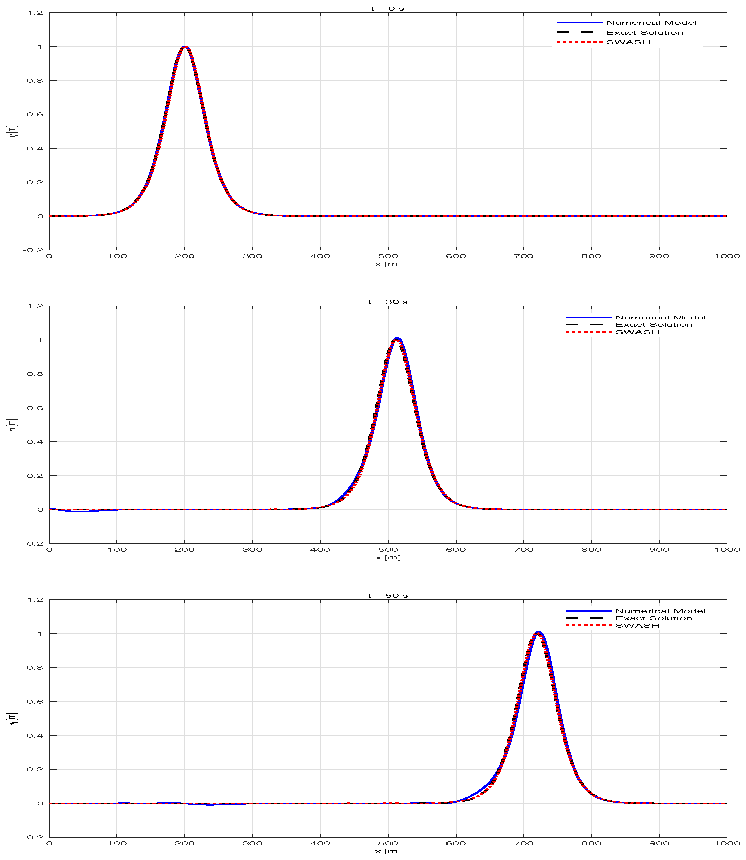
5.1. Solitary Waves Propagate over a Flat Bottom
In this subsection, we present a benchmark test for solitary wave propagation over a flat bottom. This is a benchmark test for the dispersive and nonlinear waves. For computation, a channel with
m long and
m water depth is considered. The left and right absorbing boundaries are applied. The initial wave is located at
and has the following surface profile
with
, and
. For numerical computation, we choose
and
. We compare the numerical solution to the exact solution written as:
Owing to the balance between nonlinearity and dispersion, in
Figure 5, we can see that the solitary waves travel with the correct speed, constant amplitude, and conserved shape. We plot the numerical result together with the analytical solution and SWASH result and they show a good comparison.
5.2. Solitary Waves Run up on a Sloping Beach
This section presents two benchmark tests to examine the profile of solitary waves propagate to a sloping area for the non-breaking and breaking case. The breaking criteria are based on the ratio of amplitude and water depth
, as stated in [
6], and the wave parameter for the breaking simulations is based on experimental data in that paper. The initial waves have the same profile as used in Synolakis’ experiment [
6]. This experiment was conducted at 31.73 m length, 60. 96 cm depth, and 39.97 cm width wave tank. Since the length is much longer than the width, we could use this experimental data to validate a one-dimensional problem. We use a simulation set-up where the bathymetry is a flat bottom connected to a sloping beach with the beach slope is 1:19.85. The initial condition is defined in the flat bottom area as
where
A is wave height,
is undisturbed water depth,
g is gravity acceleration,
is wave crest position, and
. This initial condition causes solitary waves to propagate to the beach on the right side. For this simulation, we set
and
. We perform two simulations which are the non-breaking case
and the breaking case
. We choose
and
to handle the moving boundary at the shoreline. In this simulation, the wet and dry procedure is applied.
We will start with a small normalized wave height
. The result is summarized in
Figure 6 which shows the comparison between the experimental measurements (dots), the hydrostatic model results [
8] (dash line), and the two-layer non-hydrostatic model results (solid line). The comparison is noticed at four different times, at
,
,
, and
. Both of the numerical results are similar and both of them are in a good agreement with the experimental data.
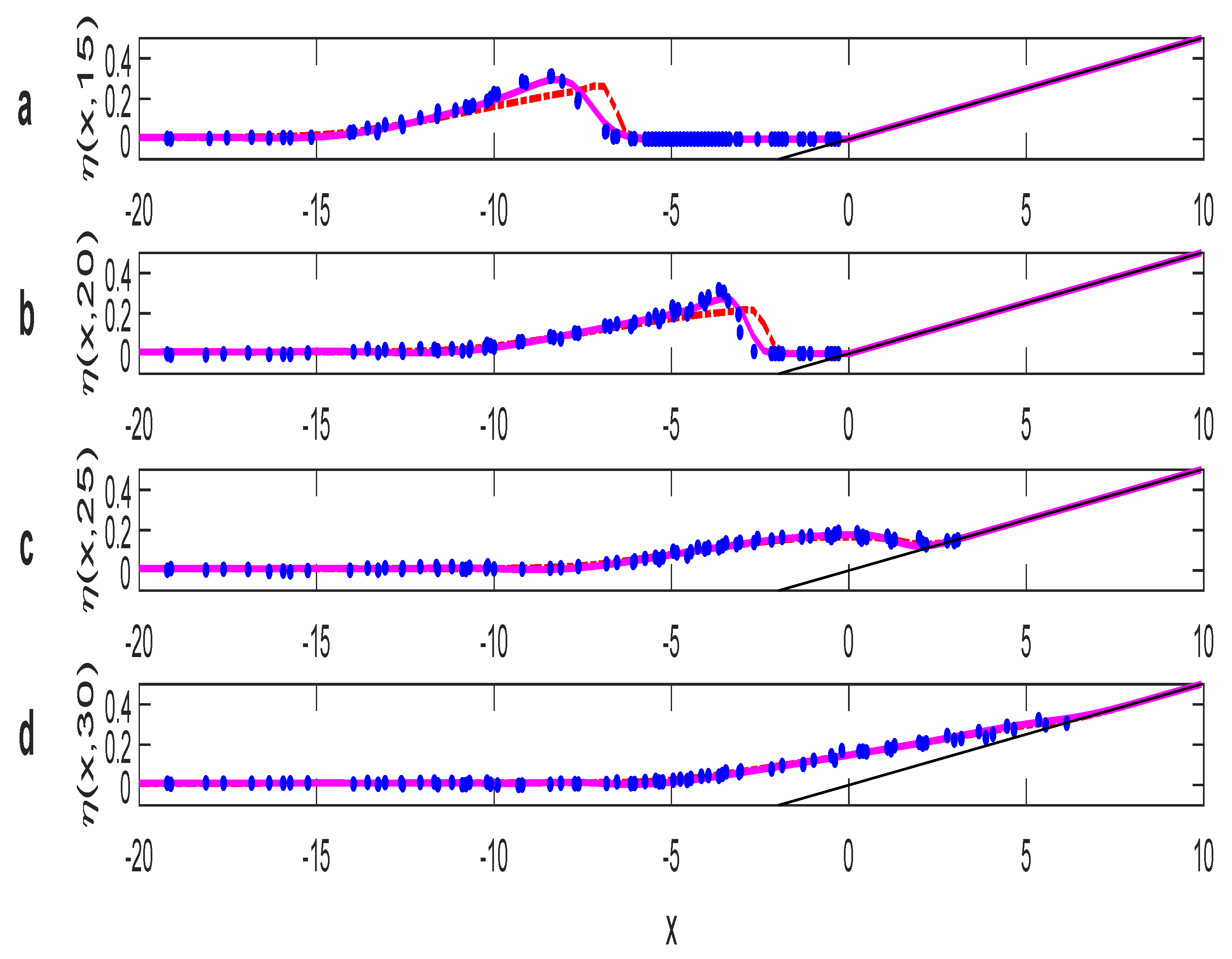
The next simulation is performed for larger normalized wave height, i.e,
. Here, the surface profiles are captured at
,
,
, and
. The comparison between laboratory experiment, the hydrostatic model, and the two-layer non-hydrostatic simulation is shown in
Figure 7.
As shown in
Figure 7, the hydrostatic model produces wave speeds that are faster than the experiment results. Implementing the non-hydrostatic model will produce better propagation speed than the hydrostatic model. Error comparison between hydrostatic and non-hydrostatic model at
and
is shown in
Table 1.
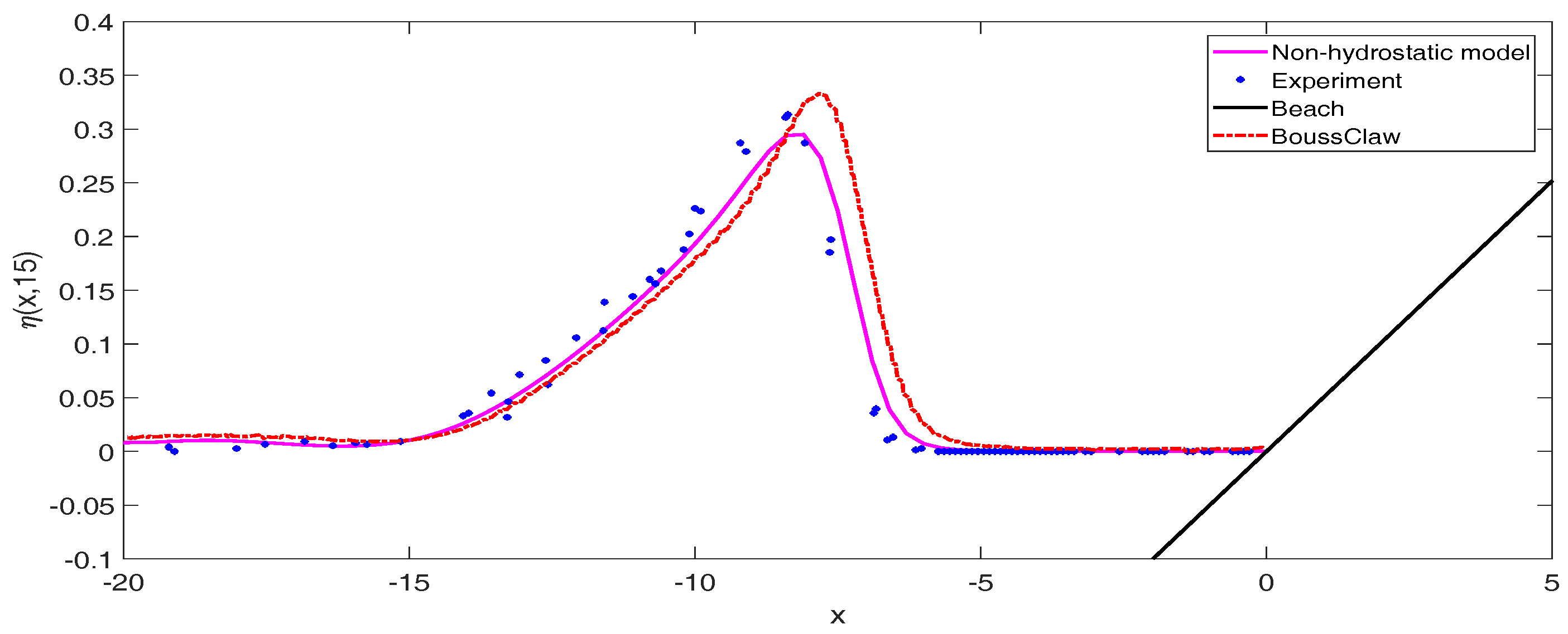
Next, we also compare our numerical model with BoussClaw numerical model as shown in
Figure 8. BoussClaw is an extension of GeoClaw (part of Clawpack developed by LeVeque [
27]) which solves the Boussinesq-type model. Both numerical models are in a good agreement with the experimental data, yet, the non-hydrostatic model produces a better approximation.
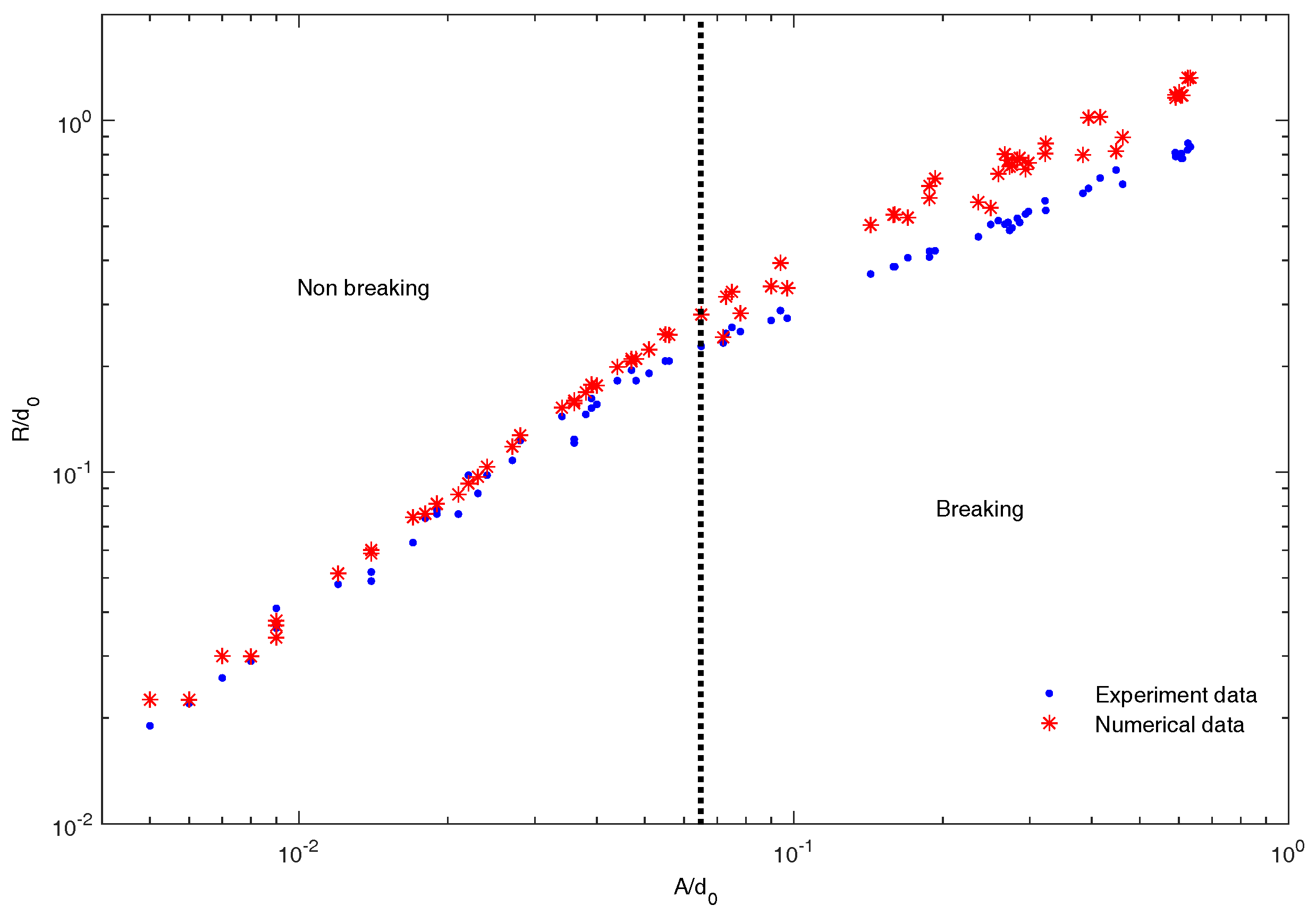
5.3. Run-up Height of Solitary Waves
In this section, the two-layer non-hydrostatic scheme will be implemented to measure the maximum run-up of solitary waves over a sloping beach. We conduct several simulations with different depth and wave height, using the same bathymetry and initial condition as shown in the previous simulation. The value
in initial condition changes with different wave height, because solitary waves with different height have different “wave length”. The value of
is chosen so that the solitary hump is on the flat bottom area. In this simulation we choose
as suggested by [
6], where
is the distance of wave crest from the toe of the beach. It is to assure that all the solitary waves propagate with the same relative distance to the beach. The experimental data in [
6] were used to be compared with our model. The water depth ranged from 6.25 cm to 38.32 cm and the wave height ratio
ranged from 0.005 to 0.633. As stated in [
6], the wave breaks during run-up when
. Run-up height for different wave height is presented in
Figure 9. Compared to the experimental data, the run-up height produced by our scheme is good enough (the average error is less than 12%) for solitary waves with the non-breaking case. For solitary waves with the breaking case, run-up height that is produced by our scheme is higher than experimental data. Nevertheless, from our numerical results, we can conclude that the relative run-up height increases as the relative wave height increases, which is confirmed by the experimental data.
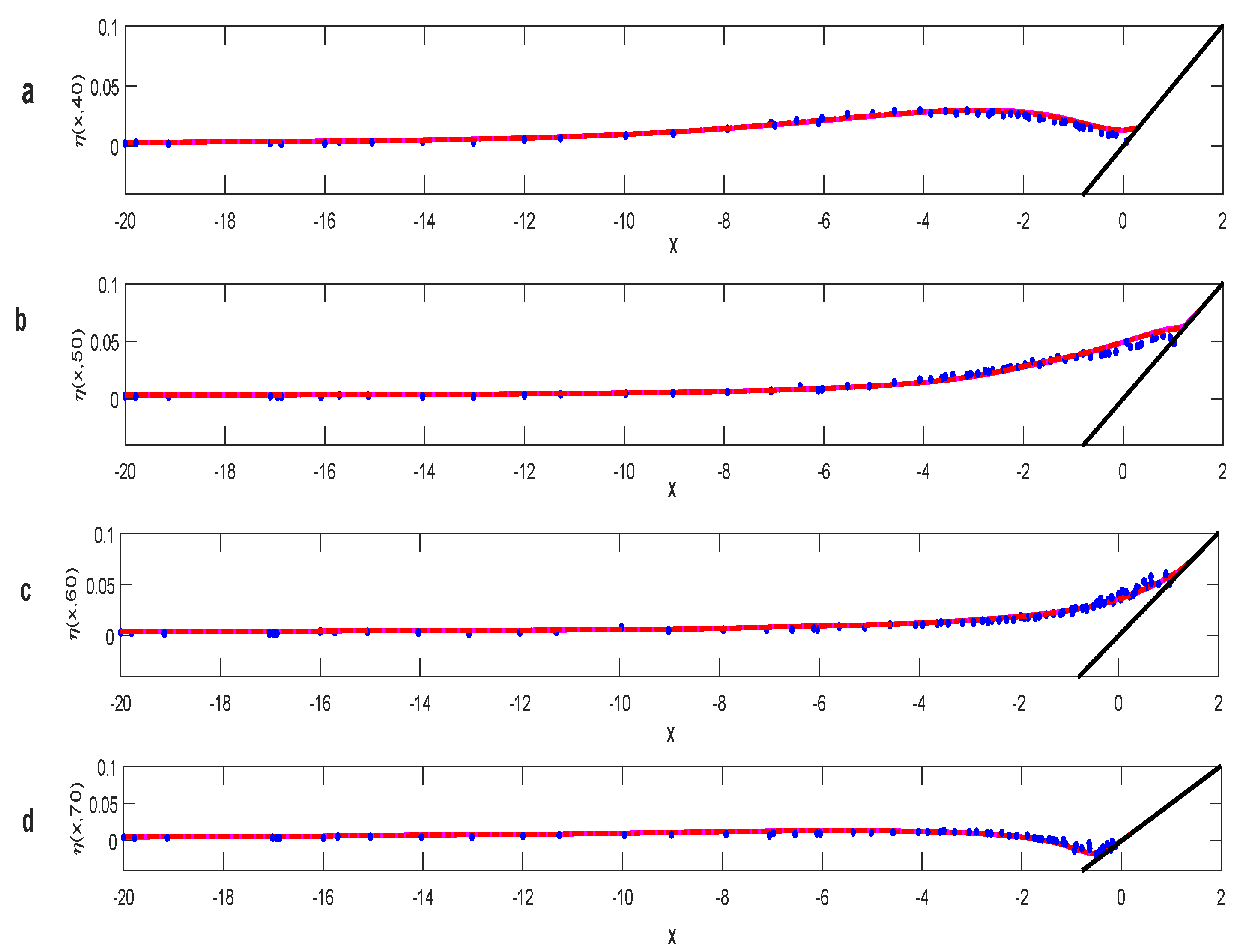
5.4. Solitary Waves Propagation over a Sloping Beach with Reefs
Here, we implement our numerical scheme to simulate wave run-up over a sloping beach with a fringing reef. This simulation offers a challenge for researchers who are working on numerical mathematics field because the existence of reef over a sloping beach makes the surf-zone processes more complex. The complexities are in describing the moving waterlines in the dry area and the breaking waves phenomenon. Therefore, a complete dispersive and nonlinear numerical scheme is not enough to simulate this case, so we need to include a correct wet-dry procedure.
In O.H. Hinsdale Wave Research Laboratory of Oregon State University, [
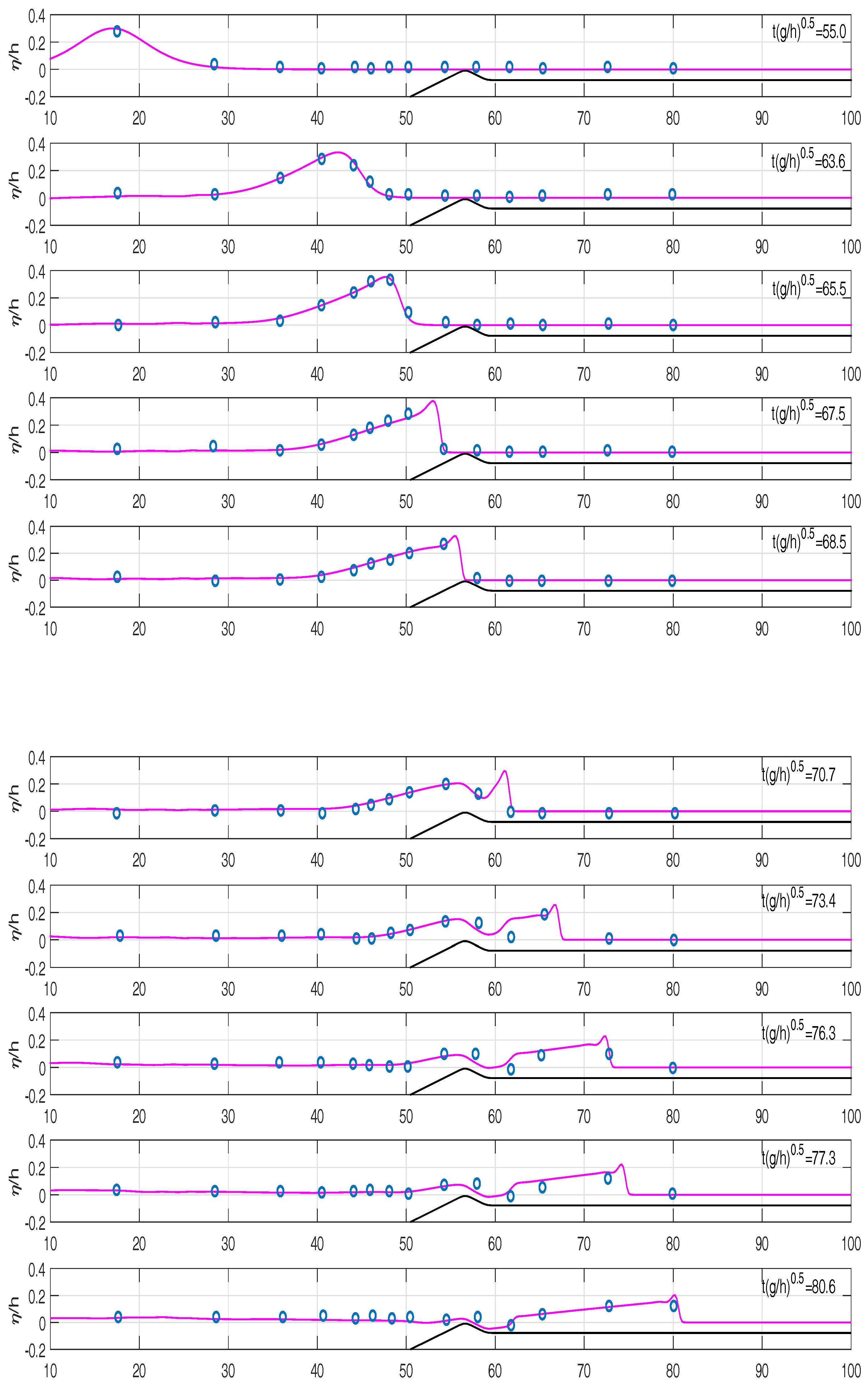
28] has investigated the transformation of solitary waves over a fringing reef under wet and dry flat conditions. He has done several experiments with different set-ups. Here, we choose two set-ups with different reef configurations and scales to demonstrate and validate our numerical model. For the first test case, the fringing reef is in a 40 m long flume with 1.0 m water depth over a sloping slope 1/5. For the computation, we choose the spatial grid and time step as
and
, respectively. The initial condition is calm water. The left boundary is a solitary wave with
, and the right boundary is a vertical wall as in the experiment. A good agreement given by the comparison of our numerical results and the measured surface elevation along the flume is shown in
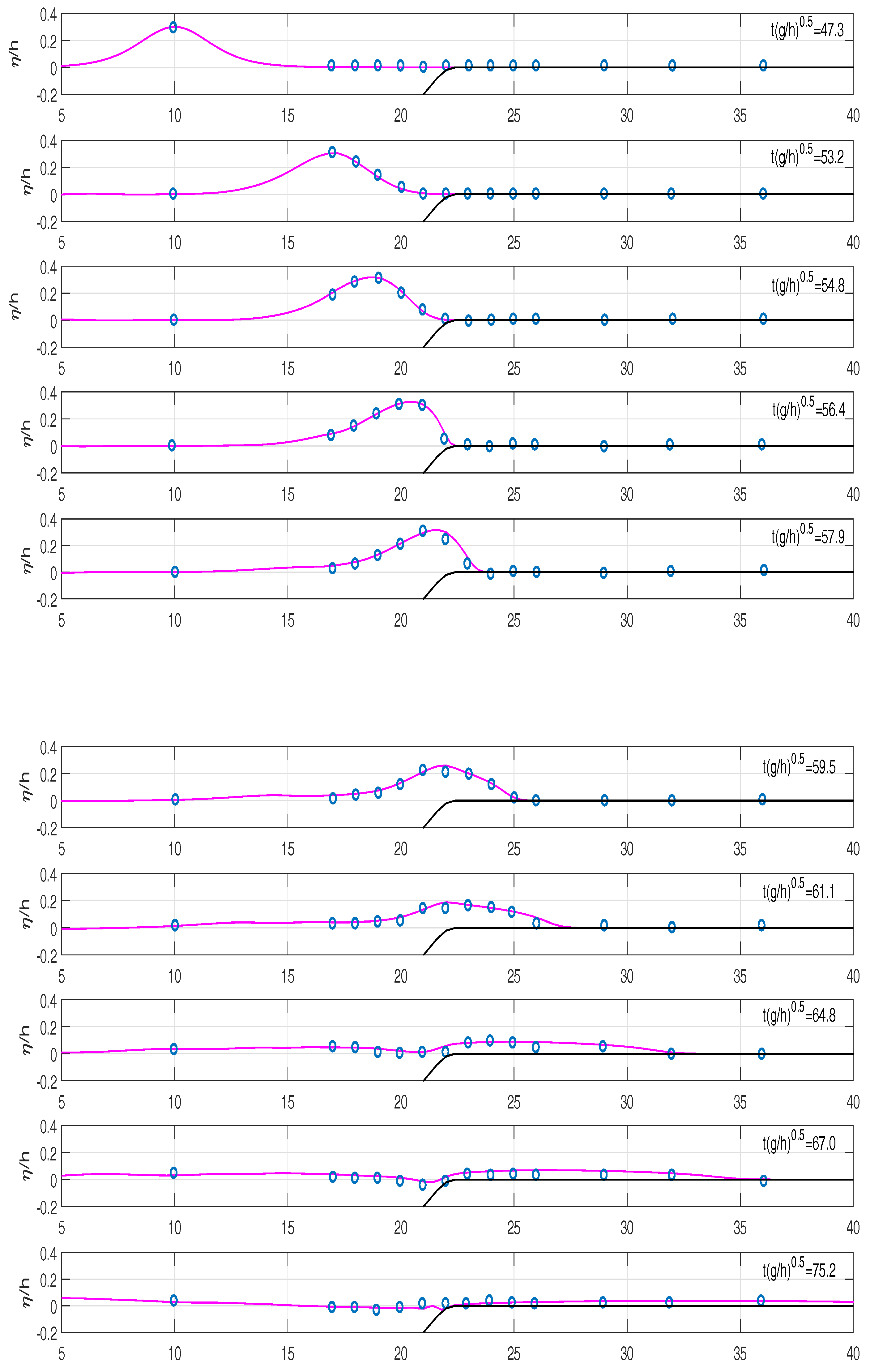
Figure 10.
The second test involves a fringing reef with a 1/12 slope and a 0.2 m high reef crest in a 100 m long and 2.56 m deep flume. The grid size and time step are
and
. The comparison between the computed and measured surface elevations for
is presented in
Figure 11. When the solitary waves propagate over the slope starting at
, the waves begin to shoal and then we see the appearance of a bore on the reef crest as the bore propagates and attenuates over time. This test case demonstrates the balance between dispersion and nonlinearity with the hydraulic jump near the shock.
5.5. Run-up Simulation Using Simplified Aceh Bathymetry
Finally, this numerical model is implemented to simulate wave run-up on simplified Aceh bathymetry. Aceh is one of the worst affected areas by the 2004 Indian Ocean tsunami. We use the same bathymetry data as mentioned in [
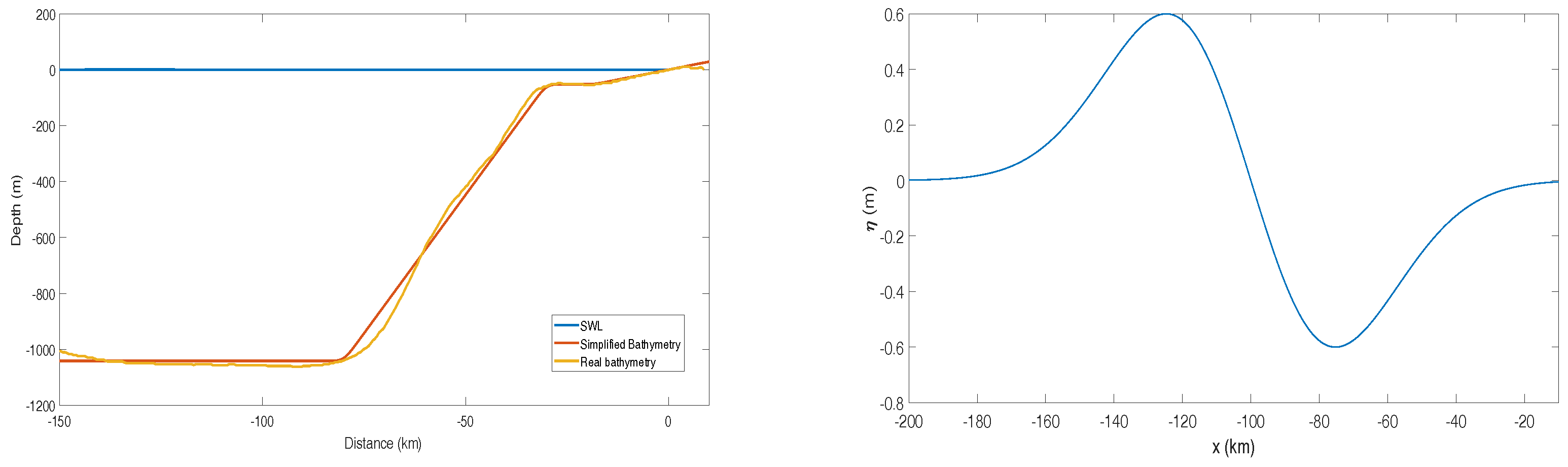
29] which located on the west coast of Aceh. Its location is about 100 km from the epicenter of the earthquake. We simplify the bathymetry using linear piecewise function as follows.
Based on the report in [
30], we use the leading depression N-waves with the wave amplitude of 0.6 m as initial waves, defined as follows.
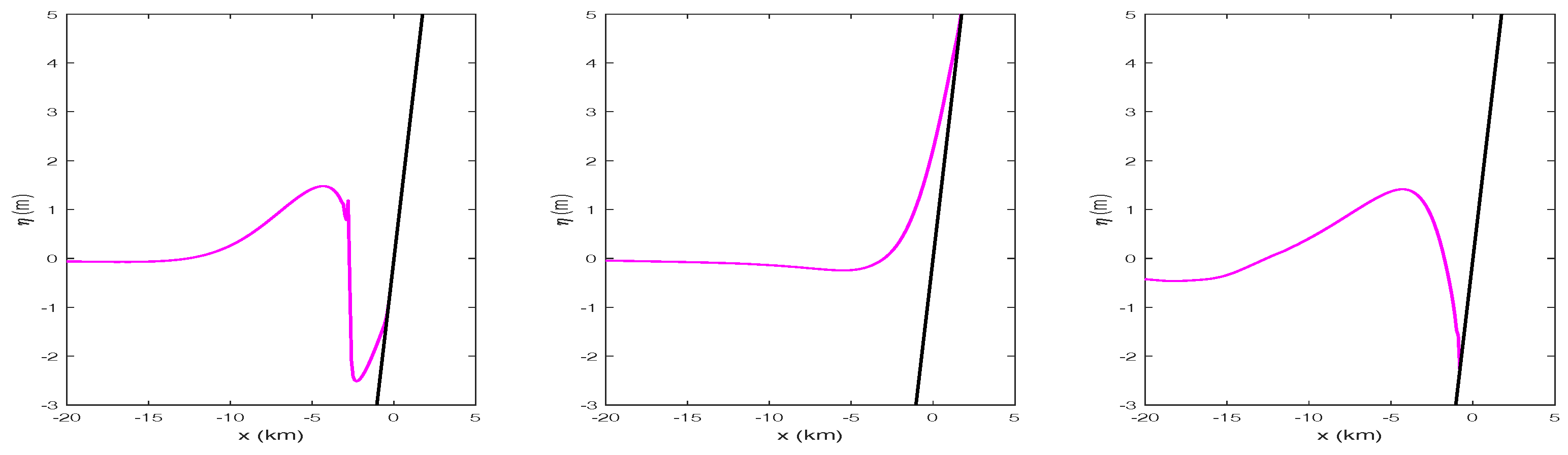
Figure 12 shows the bathymetry and the initial waves. The simplified bathymetry is close enough with the real one. The simulation is conducted for
and the dynamics of moving shoreline are shown in
Figure 13. Based on the simulation, the waves will arrive at the coastal area about 46 minutes. According to the tsunami travel time map by NOAA [
31], the arrival time of the first wave on the west coast of Aceh is about up to one hour which is consistent with our numerical result. From the simulation, the maximum run-up is 8.02 m. Using Equation (
50), the inundation area is about 2.8 km.


