Three-Stage Sequential Estimation of the Inverse Coefficient of Variation of the Normal Distribution

Abstract

This paper sequentially estimates the inverse coefficient of variation of the normal distribution using Hall’s three-stage procedure. We find theorems that facilitate finding a confidence interval for the inverse coefficient of variation that has pre-determined width and coverage probability. We also discuss the sensitivity of the constructed confidence interval to detect a possible shift in the inverse coefficient of variation. Finally, we find the asymptotic regret encountered in point estimation of the inverse coefficient of variation under the squared-error loss function with linear sampling cost. The asymptotic regret provides negative values, which indicate that the three-stage sampling does better than the optimal fixed sample size had the population inverse coefficient of variation been known.

1. Introduction

Let $X_1,X_2,\dots$ be a sequence of independent and identically distributed IID random variables from a normal distribution $N\left(\mu ,{\sigma }^2\right)$ with mean $\mu \in ℝ$ and variance ${\sigma }^2\in {ℝ}^{+}$, where both parameters are finite but unknown. The population coefficient of variation is the population standard deviation divided by the population mean that is $\sigma /\mu$, $\mu \ne 0$, mostly presented as a percentage. It is useful when we seek relative variability rather than the absolute variability. It is a dimensionless quantity, which enables researchers to compare different distributions, regardless of their measurable units. Such practicality makes it widely used in different areas of science, such as engineering, finance, economics, medicine, and others. Nairy and Rao [1] conducted a survey of several applications in engineering, business, climatology, and other fields. Ahn [2] used the coefficient of variation to predict the unknown number of flaw trees, while Gong and Li [3] used it to estimate the strength of ceramics. Faber and Korn [4] applied the measure in the mean synaptic response of the central nervous system. Hammer et al. [5] used the measure to test the homogeneity of bone samples in order to determine the effect of external treatments on the properties of bones. Billings et al. [6] used it to study the impact of socioeconomic status on hospital use in New York City. In finance, Brief and Owen [7] used the coefficient of variation to evaluate the project risks considering the rate of return as a random variable. Pyne et al. [8] used the measure to study the variability of the competitive performance of Olympic swimmers. In health sciences, see Kelley [9] and Gulhar et al. [10].

The disadvantage of the measure lies in the singularity point $\mu =0$. Therefore, it is preferable to work with the reciprocal of the measure, inverse coefficient of variation, $\theta =\mu /\sigma$ defined over $ℝ$. The inverse coefficient of variation is equal to the signal-to-noise ratio, which measures the signal strength relative to background noise. In quality control, it represents the magnitude of the process mean compared to its variation. In other words, it quantifies how much signal has been corrupted by noise, see McGibney and Smith [11]. In finance, it is called Sharpe’s index, which measures portfolio performance, for example, see Knight and Satchell [12].

Having observed a random sample $X_1,X_2,\dots ,X_n$ of size $\left(n\ge 2\right)$ from the normal population, we continue to use both ${\overline{X}}_n$ and $S_n$ as the sample mean and the sample standard deviation point estimates of the normal distribution mean $\mu$ and standard deviation $\sigma$, respectively. Consequently, we define the sample inverse coefficient of variation ${\widehat{\theta }}_n={\overline{X}}_n/S_n$.

Hendricks and Robey [13] studied the sampling distribution of the coefficient of variation. Koopmans et al. [14] showed that without any prior restriction to the range of the population mean, it is impossible to obtain confidence intervals for the population coefficient of variation that have finite length with a probability one, uniformly for all values of $\mu and\sigma$ except by using purely sequential procedure. Rao and Bhatta [15] approximate the distribution function of the sample coefficient of variation using the Edgeworth series to obtain a more accurate large-sample test for the population coefficient of variation under normality. McKay [16] derived a confidence interval for the population coefficient of variation, which is based on the chi-squared distribution. He found that the constructed confidence interval works well when the coefficient of variation is less than 0.33, see Umphrey [17]. Later Vangel [18] modified McKay’s confidence interval, which shown to be closely related to McKay’s confidence interval, but is more accurate and nearly exact under normality. Miller [19] discussed the approximate distribution function of the sample coefficient of variation and proposed the approximate confidence interval for the coefficient of variation under normality. Lehmann [20] found an exact form for the distribution function of the sample coefficient of variation, which depends mainly on the non-central $t$-distribution (defined over $ℝ)$, so it is computationally cumbersome. Curto and Pino [21] studied the distribution of the sample coefficient of variation in the case of non-IID random variables.

Sharma and Krishna [22] mathematically derived an asymptotic confidence interval for the population inverse coefficient of variation without any prior assumption regarding the underline distribution. Albatineh, Kibria, and Zogheib, [23] studied the performance of their constructed confidence interval using Monte Carlo simulation. They used randomly generated data from different distributions—normal, log-normal, ${\chi }^2$ (Chi-squared-distribution), Gamma, and Weibull distributions.

Regarding sequential estimation, Chaturvedi and Rani [24] proposed a sequential procedure to construct a fixed-width confidence interval for the population inverse coefficient of variation of a normal distribution with a preassigned coverage probability. They mathematically showed that the proposed procedure attains asymptotic efficiency and consistency in the sense of Chow and Robbins [25]. Chattopadhyay and Kelley [26] used the purely sequential procedure [25] to estimate the population coefficient of variation of the normal distribution under a squared-error loss function using a Nagar-type expansion.

Yousef and Hamdy [27] utilized Hall’s three-stage sampling procedure to estimate the population inverse coefficient of variation of the normal distribution using a Monte Carlo Simulation. They found a unified stopping rule, which is a function of the unknown population variance that tackles both a fixed-width confidence interval for the unknown population mean with a pre-assigned coverage probability and a point estimation problem for the unknown population variance under a squared-error loss function with linear sampling cost. In other words, they found the asymptotic coverage probability for the population mean and the asymptotic regret incurred by estimating the population variance by the sample variance. As an application, they write FORTRAN codes and use Microsoft Developer Studio software to find the simulated coverage probability for the inverse coefficient of variation and the simulated regret. The simulation results showed that the three-stage procedure attains asymptotic efficiency and consistency in the sense of Chow and Robbins [25].

Up to our knowledge, none of the existing papers in the literature discussed the three-stage estimation of the population inverse coefficient of variation theoretically. Here, the procedure is different than in Yousef and Hamdy [27]; the stopping rule depends directly on the sample inverse coefficient of variation. We derive mathematically an asymptotic confidence interval for the population inverse coefficient of variation that has a fixed-width $2d\left(>0\right)$ and coverage probability at least $100\left(1-\alpha \right)\%$.

Moreover, we tackle a point estimation problem for the population inverse coefficient of variation using a squared-error loss function with linear sampling cost. Then we examine the capability of the constructed confidence interval to detect any potential shift that occurs in the population inverse coefficient of variation. Here, the stopping rule depends on the asymptotic distribution of the sample inverse coefficient of variation.

The Layout of the Paper

In Section 2, we present preliminary asymptotic results that facilitate finding the asymptotic distribution of the sample inverse coefficient of variation. In Section 3, we present Hall’s three-stage procedure and find the asymptotic characteristics for both the main-study phase and the fine-tuning phase. In Section 4, we find the asymptotic coverage probability for the population inverse coefficient of variation. In Section 5, we discuss the capability of the constructed interval to detect any shift in the inverse coefficient of variation. In Section 6, we find the asymptotic regret.

2. Preliminary Results

The following Corollaries are necessary to find the asymptotic distribution of the sample inverse coefficient of variation ${\widehat{\theta }}_n={\overline{X}}_n/S_n$.

Corollary 1.

Let$X_1,X_2,\dots ,X_n$be a random sample from$N\left(\mu ,{\sigma }^2\right)$. Let$S_n^2={\sum }_{i=1}^n{\left(X_i-\overline{X}\right)}^2/\left(n-1\right)$,$n\ge 2$and$\overline{X}={{\displaystyle \sum }}_1^n{X}_i/n$for$n\ge 1$. Then for all$n\ge 6,$we have

(i) 

$E\left(S_n\right)=\sigma -\frac{\sigma }{4n}+O\left(n^{-2}\right)$

(ii) 

$E\left(S_n^4\right)={\sigma }^4+\frac{2{\sigma }^4}{n}+O\left(n^{-2}\right)$

(iii) 

$E\left(S_n^{-1}\right)={\sigma }^{-1}+\frac{3{\sigma }^{-1}}{4n}+O\left(n^{-2}\right)$

(iv) 

$E\left(S_n^{-2}\right)={\sigma }^{-2}+\frac{2{\sigma }^{-2}}{n}+O\left(n^{-2}\right)$

(v) 

$E\left(S_n^{-4}\right)={\sigma }^{-4}+\frac{6{\sigma }^{-4}}{n}+O\left(n^{-2}\right)$

Proof. 

By using the fact $\frac{\left(n-1\right)}{{\sigma }^2}{S}_n^2~{\chi }^2\left(n-1\right)$ we get $E\left(S_n\right)=\sqrt{\frac{2}{n-1}}\frac{\mathsf{\Gamma }\left(\frac{n}{2}\right)}{\mathsf{\Gamma }\left(\frac{n}{2}-\frac{1}{2}\right)}\sigma$, $E\left(S_n^4\right)=\left(\frac{n+1}{n-1}\right){\sigma }^4$, $E\left(S_n^{-1}\right)=\sqrt{\frac{n-1}{2}}\frac{\mathsf{\Gamma }\left(\frac{n}{2}-1\right)}{\mathsf{\Gamma }\left(\frac{n}{2}-\frac{1}{2}\right)}{\sigma }^{-1}$, $E\left(S_n^{-2}\right)=\frac{n-1}{n-3}{\sigma }^{-2}$, and $E\left(S_n^{-4}\right)=\frac{{\left(n-1\right)}^2}{\left(n-3\right)\left(n-5\right)}{\sigma }^{-4}$, where $\mathsf{\Gamma }\left(u\right)={{\displaystyle \int }}_0^{\infty }{t}^{u-1}{e}^{-t}dt$. The asymptotic expansion of $\sqrt{\frac{2}{n-1}}\frac{\mathsf{\Gamma }\left(\frac{n}{2}\right)}{\mathsf{\Gamma }\left(\frac{n}{2}-\frac{1}{2}\right)}=1-\frac{1}{4n}+O\left(n^{-2}\right)$, the asymptotic expansion of $\sqrt{\frac{n-1}{2}}\frac{\mathsf{\Gamma }\left(\frac{n}{2}-1\right)}{\mathsf{\Gamma }\left(\frac{n}{2}-\frac{1}{2}\right)}=1+\frac{3}{4n}+O\left(n^{-2}\right)$, $\left(\frac{n+1}{n-1}\right)=1+\frac{2}{n}+O\left(n^{-2}\right)$, while the asymptotic expansion of $\frac{{\left(n-1\right)}^2}{\left(n-3\right)\left(n-5\right)}=1+\frac{6}{n}+O\left(n^{-2}\right)$. By direct substitution, we get the results. The proof is complete. □

The next corollary provides the asymptotic characteristics of ${\widehat{\theta }}_n={\overline{X}}_n/S_n$ in the case of fixed sample size $n,$ as shown in Chaturvedi and Rani [24].

Corollary 2.

For all $n\ge 8,$ as $n\to \infty$ we have

(i) 

$E\left({\widehat{\theta }}_n\right)=\theta \left(1+\frac{3}{4n}\right)+O\left(n^{-1}\right)$

(ii) 

$E\left({\widehat{\theta }}_n^2\right)={\theta }^2+\frac{1}{n}\left(1+2{\theta }^2\right)+O\left(n^{-1}\right)$

(iii) 

$Var\left({\widehat{\theta }}_n\right)=\frac{1}{n}\left(1+\frac{{\theta }^2}{2}\right)+O\left(n^{-1}\right)$

(iv) 

$E\left({\widehat{\theta }}_n^4\right)={\theta }^4+\frac{6{\theta }^2}{n}\left(1+{\theta }^2\right)+O\left(n^{-1}\right)$

(v) 

$Var\left({\widehat{\theta }}_n^2\right)=\frac{2{\theta }^2}{n}\left(2+{\theta }^2\right)+O\left(n^{-1}\right)$.

Proof. 

The proof follows from Lemma 1 and Lemma 2 in Chaturvedi and Rani [24]. □

For simplicity, let us consider $Var\left({\widehat{\theta }}_n\right)\cong \frac{{\theta }^2}{2n}$, then from the central limit theorem as $n\to \infty ,Q=\frac{\sqrt{2n}\left({\widehat{\theta }}_n-\theta \right)}{\theta }\to N\left(0,1\right)$ in distribution. To satisfy the requirement of having a confidence interval for $\theta$ that has a fixed-width $2d$ and coverage probability with at least $100\left(1-\alpha \right)\%$, we need

$$P\left(\left|\frac{\sqrt{2n}\left({\widehat{\theta }}_n-\theta \right)}{\theta }\right|\le \frac{d\sqrt{2n}}{\theta }\right)\ge 1-\alpha ,$$

From which we get,

$$n\ge n^{*}=\xi {\theta }^2,\xi =\frac{a^2}{2d^2}$$

(1)

where $a=Z_{\alpha /2}$ is the upper $\alpha /2$ cut off point of the $\mathcal{N}\left(0,1\right)$.

Since $\theta$ is unknown, then no fixed sample size procedure can achieve the above confidence interval uniformly for all $\mu ,$ and $\sigma$, see Dantzig [28]. Therefore, we resort to the three-stage procedure to estimate the unknown population inverse coefficient of variation $\theta$ via estimation of $n^{*}$.

3. Three-Stage Sequential Estimation

Hall [29,30] introduced the idea of sampling in three-stages for constructing a confidence interval for the mean of the normal distribution that has prescribed width and coverage probability. His findings motivated many researchers to utilize the procedure to generate inference for other distributions; for a complete list of research, see Ghosh, Mukhopadhyay, and Sen [31]. Others have introduced point estimation under some error loss functions or tried to improve the quality of inference like protecting the inference against type II error probability, studying the operating characteristic curve, or/and discussing the sensitivity of the three-stage sampling when the underline distribution departs away from normality. For details, see Costanzo et al. [32], Hamdy et al. [33], Son et al. [34], Yousef et al. [35], Hamdy et al. [36], and Yousef [37,38].

In the following lines, we present Hall’s three-stage procedure, as described by Hall [29,30]. The procedure based on three phases: The pilot phase, the main-study phase, and the fine-tuning phase.

The Pilot Phase: In the pilot study phase a random sample of size ($m\ge 3$) is taken from the normal distribution say, $\left(X_1,X_2,X_3,\dots ,X_m\right)$ to initiate sample measure, ${\overline{X}}_m$ for the population mean $\mu$ and $S_m$ for the population standard deviation $\sigma$. Hence, we propose to estimate the inverse coefficient of variation $\theta$ by the corresponding sample measure ${\widehat{\theta }}_m$.

The Main Study Phase: We estimate only a portion $\gamma \left(0<\gamma <1\right)$ of $n^{*}$ to avoid possible oversampling. In literature, $\gamma$ is known as the design factor.

$$N_1=max\{m,\left[\gamma \xi {\widehat{\theta }}_m^2\right]+1\}$$

(2)

where, $\left[·\right]$ means the largest integer function.

If $\ge N_1$, then we stop at this stage; otherwise, we continue to sample an extra sample of size $N_1-m$, say $\left(X_{m+1},X_{m+2},X_{m+3},\dots ,X_{N_1}\right)$, then we update the sampling measures ${\overline{X}}_{N_1},S_{N_1}$ and ${\widehat{\theta }}_{N_1}$ for the unknown population parameters, $\mu ,\sigma ,$ and $\theta ,$ respectively.

The Fine-Tuning Phase: In the fine-tuning phase, the decision to stop sampling or continue based on the following stopping rule

$$N=max\{N_1,\left[\xi {\widehat{\theta }}_{N_1}^2\right]+1\}$$

(3)

If $N_1\ge N$, sampling is terminated, else we continue to sample and an additional sample of size $N-N_1$, say $\left(X_{N_1+1},X_{N_1+2},X_{N_1+3},\dots ,X_N\right).$ Hence, we augment the previously collected $N_1$ samples with the new $N-N_1$ to update the sample estimates to ${\overline{X}}_N,S_N$ and ${\widehat{\theta }}_N$ for the unknown parameters $\mu ,\sigma ,$ and $\theta$. Upon terminating the sampling process, we propose to estimate the unknown inverse coefficient of variation $\theta$ with the fixed $2d$ confidence interval $I_N=\left({\widehat{\theta }}_N-d,{\widehat{\theta }}_N+d\right)$.

The following asymptotic results are developed under the general assumptions set forward by Hall [28] to develop a theory for the three-stage procedure, condition (A) by definition, $\xi >0$, $n^{*}\to \infty \Rightarrow$ $\lim sup\left(\frac{m}{n^{*}}\right)<\gamma$ and $\xi \left(m\right)=O\left(m^k\right)$, $k>1$.

The following Helmert’s transformation is necessary to obtain asymptotic results regarding $S_{N_1}^{2k}$ and $S_N^{2k}$ for any real number $k$. We need to express the sample variance $S_n^2$ as an average of IID random variables. To do so let

$$\{\begin{array}{c}{W}_i={{\displaystyle \sum }}_j^i(Z_j-i{Z}_{i+1})/\sqrt{i\left(i+1\right)},i=1,2,\dots ,n-1\\ W_n=n^{-1}{{\displaystyle \sum }}_{j=1}^n{Z}_j\end{array}$$

where $Z_i=\frac{X_i-\mu }{\sigma },\forall i=1,\dots ,n$. It follows that $W_i$ is IID $N\left(0,1\right)\forall i=1,2,\dots ,n$. If we set $V_i={\sigma }^2{W}_i^2$ then $V_i\sim {\sigma }^2{\chi }^2\left(1\right)$ for $\forall i=2,\dots ,n.$ From Lemma 2 of Robbins [39], it follows that $S_n^2$ and ${\overline{V}}_n={\left(n-1\right)}^{-1}{{\displaystyle \sum }}_{i=2}^n{V}_i$ are identically distributed. So, in all the proofs we use ${\overline{V}}_n$ instead of $S_n^2$, $n\ge 2$ to develop asymptotic results regarding $E\left(S_{N_1}^2\right)$ and $E\left(S_N^2\right)$.

Under condition (A),

$$P\left(N=\left(\left[\xi {\widehat{\theta }}_{N_1}^2\right]+1\right)\right)\to 1,\mathrm{and}\frac{N_1}{\gamma n^{*}}\to 1\mathrm{in}\mathrm{probability}\mathrm{as}m\to \infty .$$

From Anscombe’s [40] central limit Theorem, we have as $\xi \to \infty$,

(i)

$\sqrt{2N_1}\left({\widehat{\theta }}_{N_1}-\theta \right)\to \mathcal{N}\left(0,{\theta }^2\right)$ in distribution

(ii)

$\sqrt{N_1}\left({\widehat{\theta }}_{N_1}^2-{\theta }^2\right)\to N\left(0,2{\theta }^4\right)$ in distribution

Now, $N=\left[\xi {\widehat{\theta }}_{N_1}^2\right]+1$, except possibly on a set $\eta =\left(N_1<m{\displaystyle \cup }\xi {\widehat{\theta }}_{N_1}^2<\gamma \xi {\widehat{\theta }}_m^2+1\right)$ of measure zero. Therefore, for real $r$, we have

$$E\left(N^r\right)=E{(\xi {\widehat{\theta }}_{N_1}^2+{\beta }_{N_1})}^r+{{\displaystyle \int }}_{\eta }^{}{N}^{r}dP\Rightarrow E\left(N^r\right)=E{(\xi {\widehat{\theta }}_{N_1}^2+{\beta }_{N_1})}^r+o\left({\xi }^{r-1}\right)$$

Provided that the $r^{th}$ moment exists and as $\xi \to \infty ,{\beta }_{N_1}=\left(\xi {\widehat{\theta }}_{N_1}^2\right)-\left[\xi {\widehat{\theta }}_{N_1}^2\right]~U\left(0,1\right)$.

3.1. The Asymptotic Characteristics of the Main-Study Phase

The following theorem gives a second-order approximation regarding the $k^{th}$ moment of the sample average of the main-study phase.

Theorem 1.

For the three-stage sampling rule in Equation (2), if condition (A) holds then, as$\xi \to \infty$,

$$E\left({\overline{X}}_{N_1}^k\right)={\theta }^k{\sigma }^k+\frac{k\left(k-5\right){\theta }^{k-2}{\sigma }^k}{2\gamma n^{*}}+o\left({\xi }^{-1}\right).$$

Proof. 

We write

$$E\left({\overline{X}}_{N_1}^k\right)={\theta }^k{\sigma }^{k}E{\left(1+\frac{{{\displaystyle \sum }}_{i=1}^{N_1}{Z}_i}{\theta N_1}\right)}^k$$

Then, we expand the above expression in infinite series while conditioning on the $\sigma$–field generated by $Z_1,Z_2,\dots ,Z_m$, where $Z_i=\frac{\left(X_i-\mu \right)}{\sigma }$ are standard normal variates. Notice also that,

$$E{\left(\frac{N_1-m}{N_1}\right)}^k=o\left({\xi }^{-1}\right)\mathrm{as}\xi \to \infty .$$

Thus

$$E\left({\overline{X}}_{N_1}^k\right)={\theta }^k{\sigma }^{k}E{\left(1+\frac{{{\displaystyle \sum }}_{i=1}^m{Z}_i}{\theta N_1}\right)}^k.$$

Consider the first three terms in the infinite Binomial series and expand ${\left(N_1\right)}^{-k}$ in Taylor series around $\gamma n^{*}$ and taking the expectation all through, the statement of Theorem 1 is immediate. □

Special cases of Theorem 1, when $k=1$ and $k=2$, provide

$$E\left({\overline{X}}_{N_1}\right)=\mu -\frac{2\sigma }{\theta \gamma n^{*}}+o\left({\xi }^{-1}\right)$$

(4)

$$E({\overline{X}}_{N_1}^2)={\mu }^2-\frac{3{\sigma }^2}{\gamma n^{*}}+o\left({\xi }^{-1}\right)$$

(5)

It follows from Equations (4) and (5),

$$Var\left({\overline{X}}_{N_1}\right)=\frac{{\sigma }^2}{\gamma n^{*}}+o\left({\xi }^{-1}\right)$$

(6)

Theorem 2 below gives the $k^{th}$ moment of the three-stage sample variance of the main-study phase.

Theorem 2.

For the three-stage sampling rule in Equation (2), if condition (A) holds then, for real k and as$\xi \to \infty$

$$E\left(S_{N_1}^{2k}\right)={\sigma }^{2k}+\frac{k\left(k-1\right){\sigma }^{2k}}{\gamma n^{*}}+o\left({\xi }^{-1}\right).$$

Proof. 

First, write $E\left(S_{N_1}^{2k}\right)=E({\overline{V}}_{N_1}^{2k}$). Hence, we condition on the $\sigma -$ field generated by $V_1$, $V_2$, $V_3$,…, $V_{m-1}$ write

$$E\left(S_{N_1}^{2k}\right)=E{\left(N_1-1\right)}^{-k}E{({{\displaystyle \sum }}_{i=1}^{m-1}{V}_i+{{\displaystyle \sum }}_{i=m}^{N_1-1}{V}_i)}^k|V_1,V_2,V_3,\dots ,V_{m-1}.$$

Then we expand the binomial term as an infinite series as

$$E\left(S_{N_1}^{2k}\right)=E\{{\left(N_1-1\right)}^{-k}{{\displaystyle \sum }}_{j=0}^{\infty }\zeta \left(k,j\right){({{\displaystyle \sum }}_{i=1}^{m-1}{V}_i)}^{k-j}E{({{\displaystyle \sum }}_{i=m}^{N_1-1}{V}_i)}^j\}|V_1,V_2,V_3,\dots ,V_{m-1}$$

where $\zeta \left(k,j\right)=1$, when $j=0,$ and $\zeta \left(k,j\right)=\frac{{{\displaystyle \prod }}_{r=1}^j(k-r+1)}{j!}$ for $j=1,2,3,\dots$

Conditioning on $V_1,V_2$, $V_3$,…, $V_{m-1}$ the random variable (${{\displaystyle \sum }}_{i=m}^{N_1-1}{V}_i)$ is distributed according to ${\sigma }^2{\chi }_{N_{1-m}}^2$ and therefore $E{({{\displaystyle \sum }}_{i=m}^{N_1-1}{V}_i)}^j={\left(N_1-m\right)}^j{\sigma }^{2j}\left(1+O\left(N_1{}^{-1}\right)\right).$ Thus,

$$E\left(S_{N_1}^{2k}\right)={\sigma }^{2k}E{\left(1+\frac{{{\displaystyle \sum }}_{i=1}^{m-1}{w}_i}{N_1-1}\right)}^k+o\left({\xi }^{-1}\right)$$

where $w_i=\frac{V_i-{\sigma }^2}{{\sigma }^2}$, with $E\left(w_i\right)=0,$ and $Var\left(w_i\right)=2$.

Consider the first three terms in the infinite expansion of the above expression in addition to a remainder term, and then we have

$$E\left(S_{N_1}^{2k}\right)={\sigma }^{2k}+{\sigma }^{2k}kE\left(\frac{{{\displaystyle \sum }}_{i=1}^{m-1}{w}_i}{N_1-1}\right)+\frac{1}{2}{\sigma }^{2k}k\left(k-1\right)E{\left(\frac{{{\displaystyle \sum }}_{i=1}^{m-1}{w}_i}{N_1-1}\right)}^2+E\left(R\left(w\right)\right).$$

Recall $E\left(R\left(w\right)\right)$ = $ME{\left(\frac{{{\displaystyle \sum }}_{i=1}^{m-1}{w}_i}{N_1-1}\right)}^3$, where $M$ is a generic constant. Since $-1\le$ $N_1-1$, we have

$$E\left(R\left(w\right)\right)=ME{\left(\frac{{{\displaystyle \sum }}_{i=1}^{m-1}{w}_i}{m-1}\right)}^3=M{\left(m-1\right)}^{3}E{({\overline{V}}_m-{\sigma }^2)}^3/{(m-1)}^3=ME{\left({\overline{V}}_m-{\sigma }^2\right)}^3=0.$$

Consider the second term ${\sigma }^{2k}kE\left(\frac{{{\displaystyle \sum }}_{i=1}^{m-1}{w}_i}{N_1-1}\right)$, and expand ($N_1-1{)}^{-1}$ in Taylor series

$${\left(N_1-1\right)}^{-1}={(\gamma n^{*})}^{-1}-\left(N_1-\gamma n^{*}\right){(\gamma n^{*})}^{-2}+\left(1/2\right){(N_1-\gamma n^{*})}^2{(\rho )}^{-3},$$

where $\rho$ is a random variable lies between $N_1$ and $\gamma n^{*}$. It is not hard to show that

$$E\{({{\displaystyle \sum }}_{i=1}^{m-1}{w}_i){(N_1-\gamma n^{*})}^2{(\rho )}^{-3}\}=o\left({\xi }^{-1}\right).$$

We omit details for brevity.

$${\sigma }^{2k}kE\left(\frac{{{\displaystyle \sum }}_{i=1}^{m-1}{w}_i}{N_1-1}\right)={\sigma }^{2k-2}kmE\{\left({\overline{V}}_m-{\sigma }^2\right)\{{(\gamma n^{*})}^{-1}-m\left({\overline{X}}_m^2{\overline{V}}_m^{-1}-{\theta }^2\right)/{\theta }^2\left(\gamma n^{*}\right)+\mathrm{o}\left({\xi }^{-1}\right)\}\}$$

$${\sigma }^{2k}kE\left(\frac{{{\displaystyle \sum }}_{i=1}^{m-1}{w}_i}{N_1-1}\right)=-\frac{{\sigma }^{2k-2}k{m}^2}{{\theta }^2\left(\gamma n^{*}\right)}\{-E\left({\overline{X}}_m^2{\overline{V}}_m^{-1}{\overline{V}}_m\right)+{\sigma }^{2}E\left({\overline{X}}_m^2{\overline{V}}_m^{-1}\right)\}+o\left({\xi }^{-1}\right)=o\left({\xi }^{-1}\right)$$

Likewise, we recall the third term and expand ($N_1-1{)}^{-2}$ in Taylor series we get

$$\frac{1}{2}{\sigma }^{2k}k\left(k-1\right)E{\left(\frac{{{\displaystyle \sum }}_{i=1}^{m-1}{w}_i}{N_1-1}\right)}^2=\frac{{\sigma }^{2k}k\left(k-1\right)}{\left(\gamma n^{*}\right)}.$$

Finally, collect terms, and the statement of Theorem 2 is complete. □

A particular case for Theorem 2 at $k=-\frac{1}{2}$ and $k=-1$ are as follows

$$E\left(S_{N_1}^{-1}\right)={\sigma }^{-1}+\frac{3}{4\gamma n^{*}}{\sigma }^{-1}+o\left({\xi }^{-1}\right)$$

(7)

and

$$E\left(S_{N_1}^{-2}\right)={\sigma }^{-2}+\frac{2}{\gamma n^{*}}{\sigma }^{-2}+o\left({\xi }^{-1}\right)$$

(8)

Asymptotic results of the sample inverse coefficient of variation of the main-study phase Theorems 1, and 2, above provided the following approximate upper bound estimates

Corollary 3.

For the three-stage sampling rule in Equation (2), if condition (A) holds, then as $\xi \to \infty$ we have

(i) 

$E\left({\widehat{\theta }}_{N_1}\right)=\theta +\frac{3\theta }{4\gamma n^{*}}+o({\xi }^{-1})$

(ii) 

$E\left({\widehat{\theta }}_N^2{}_1\right)={\theta }^2+\frac{2{\theta }^2}{\gamma n^{*}}+o\left({\xi }^{-1}\right)$

(iii) 

$Var({\widehat{\theta }}_{N_1})=\frac{{\theta }^2}{2\gamma n^{*}}+o({\xi }^{-1})$

Proof. 

The proof of (i), and (ii) follows immediately from Equations (4), (5), (7) and (8). Part (iii) follows from (i) and (ii). The proof is complete. □

3.2. The Asymptotic Characteristics of the Fine-Tuning Phase

Recall the representation of $N$ and write

$$\begin{array}{c}E\left(N\right)=E\xi {\widehat{\theta }}_{N_1}^2+E\left({\beta }_{N_1}\right)+o\left(1\right)=n^{*}+\frac{4+\gamma }{2\gamma }+o\left(1\right)\\ E(N^2)=n^{*}+6{\gamma }^{-1}{n}^{*}+o\left(\xi \right)\end{array}$$

(9)

and

$$Var\left(N\right)=\frac{\left(2-\gamma \right)}{\gamma }{n}^{*}+o\left(\xi \right)$$

(10)

Theorem 3 gives a second-order approximation of a continuously differentiable and bounded real-valued function of $N.$

Theorem 3.

If condition (A) holds and ($𝒽>$ 0) be a real-valued continuously differentiable and bounded function, such that $\underset{n>m}{\sup }\left|h^{‴}\left(n\right)\right|=o\left|h^{‴}\left(n^{*}\right)\right|$, then

$$E𝒽\left(N\right)=𝒽\left(n^{*}\right)+\left(\frac{4+\gamma }{2\gamma }\right){𝒽}^{\prime }\left(n^{*}\right)+\left(\frac{2-\gamma }{2\gamma }\right)n^{*}{𝒽}^{″}\left(n^{*}\right)+o\left({\xi }^2{𝒽}^{‴}\left(n^{*}\right)\right).$$

Proof. 

The proof follows by expanding $h\left(N\right)$ around $n^{*}$ using the Taylor series. Then utilizing Equations (9) and (10) in the expansion, we get the result. □

Theorem 4.

For the three-stage sampling rule in Equation (3), if Condition A holds then, as $\xi \to \infty$,

$$E\left({\overline{X}}_N^k\right)={\theta }^k{\sigma }^k+\frac{k{\theta }^{k-2}{\sigma }^k\{\gamma \left(k-1\right)-4\}}{2n^{*}}+o\left({\xi }^{-1}\right).$$

Proof. 

First, write

$$E\left({\overline{X}}_N^k\right)={\theta }^k{\sigma }^{k}E{\left(1+\frac{{{\displaystyle \sum }}_{i=1}^N{Z}_i}{N\theta }\right)}^k,$$

then write down the binomial expression as an infinite series as

$$E{\left(1+\frac{{{\displaystyle \sum }}_{i=1}^N{Z}_i}{N\theta }\right)}^k={{\displaystyle \sum }}_{j=0}^{\infty }\zeta \left(k,j\right)E\{{({{\displaystyle \sum }}_{i=1}^N{Z}_i)}^j{\left(N\theta \right)}^{-j}\},$$

where, $\zeta \left(k,j\right)=1$, when $j=0,$ and $\zeta \left(k,j\right)=\frac{{{\displaystyle \prod }}_{r=1}^j(k-r+1)}{j!}$ for $j=1,2,3,\dots$

Now, conditioning on the $\sigma -$ field generated by $Z_1,Z_2,Z_3,\dots ,Z_{N_1}$ and we write the conditional sum ${({{\displaystyle \sum }}_{i=1}^N{Z}_i)}^j|Z_1,Z_2,Z_3,\dots ,Z_{N_1}$ $=$ ${({{\displaystyle \sum }}_{i=1}^{N_1}{Z}_i+{{\displaystyle \sum }}_{i=N_1+1}^N{Z}_i)}^j|Z_1,Z_2,Z_3,\dots ,Z_{N_1}$ as a binomial expansion, then take the conditional expectation we get

$$E\left({\overline{X}}_N^k\right)={\theta }^k{\sigma }^{k}E{\left(1+\frac{{{\displaystyle \sum }}_{i=1}^{N_1}{Z}_i}{N\theta }\right)}^k,$$

where $Z_i$ are standard normal variates.

$\left({{\displaystyle \sum }}_{i=N_1}^N{Z}_i\right)$|$X_1$, $X_2,X_3,\dots ,X_{N_1}$ is distributed $N\left(\mu =0,{\sigma }^2=N-N_1\right)$

Therefore, ${\left({{\displaystyle \sum }}_{i=N_1}^N{Z}_i/\sqrt{(N-N_1}\right)}^2$|$X_1,X_2,X_3,\dots ,X_{N_1}$ is distributed as ${\chi }_1^2$. Hence,

$$E{\left(\frac{{{\displaystyle \sum }}_{i=N_1}^N{Z}_i}{N}\right)}^k|X_1,X_2,X_3,\dots ,X_{N_1}\approx E{\left(\frac{\sqrt{N-N_1}}{N}\right)}^k=0$$

as $\xi \to \infty .$ and finally, we have $E\left({\overline{X}}_N^k\right)={\theta }^k{\sigma }^{k}E$ ${\left(1+\frac{{{\displaystyle \sum }}_{i=1}^{N_1}{Z}_i}{N\theta }\right)}^k$, where $Z_i$ are standard normal variates.

Consider the first three terms and the remainder in the infinite series, expand $N^{-1}$, and $N^{-2}$ and take the expectation through, then the statement of Theorem 4 is proved. It is not hard to prove the remainder term is of order $o\left({\xi }^{-1}\right)$. We omit any further details. □

Special cases of Theorem 4, for $k=1,2,and4$ are particularly important

$$E\left({\overline{X}}_N\right)=\mu -\frac{2\sigma }{\theta n^{*}}+o\left({\xi }^{-1}\right)$$

(11)

$$E\left({\overline{X}}_N^2\right)={\mu }^2+\frac{\left(\gamma -4\right){\sigma }^2}{n^{*}}+o\left({\xi }^{-1}\right)$$

(12)

$$E\left({\overline{X}}_N^4\right)={\mu }^4+\frac{2\left(3\gamma -4\right){\theta }^2{\sigma }^4}{n^{*}}+o\left({\xi }^{-1}\right)$$

(13)

Theorem 5 gives a second-order approximation for the $k^{th}$ moment of the fine-tuning sample variance.

Theorem 5.

For the three-stage sampling rule in Equation (3), if condition (A) holds then, for real k as $\xi \to \infty$

$$E\left(S_N^{2k}\right)={\sigma }^{2k}+\frac{\gamma {\sigma }^{2k}k\left(k-1\right)}{n^{*}}+o\left({\xi }^{-1}\right).$$

Proof. 

The proof of Theorem 5 can be justified along the lines of the proof of Theorem 4 if we condition on the $\sigma -$ field generated by $V_1,V,V_3,\dots ,V_{N_1}$ and expand ${({{\displaystyle \sum }}_{i=1}^{N_1}{V}_i+{{\displaystyle \sum }}_{i=N_1}^N{V}_i)}^k$ as an infinite series, to get,

$$E\left({\overline{V}}_N^k\right)=E\left({{\displaystyle \sum }}_{j=0}^{\infty }\zeta \left(k,j\right){({{\displaystyle \sum }}_{i=1}^{N-1}{V}_i)}^{k-j}E{({{\displaystyle \sum }}_{i=N_1}^{N-1}{V}_i)}^j\right)|V_1,V,V_3,\dots ,V_{N_1},$$

where, $\zeta \left(k,j\right)=1$, when $j=0,$ and $\zeta \left(k,j\right)=\frac{{{\displaystyle \prod }}_{r=1}^j(k-r+1)}{j!}$ for $j=1,2,3,\dots$

The random sum $\left({{\displaystyle \sum }}_{i=N_1}^{N-1}{V}_i\right)|V_1,V_2,V_3,\dots ,V_{N_1}$ is distributed as a ${\sigma }^2{\chi }_{\left(N-N_1\right)}^2$ and

$$E{({{\displaystyle \sum }}_{i=N_1}^N{V}_i)}^j|V_1,V,V_3,\dots ,V_{N_1}={(N-N_1)}^j{\sigma }^{2j}\left(1+O\left(N^{-1}\right)\right).$$

Thus, $E\left({\overline{V}}_N^k\right)={\sigma }^{2k}$ + ${\sigma }^{2k}E{\left(1+\frac{{{\displaystyle \sum }}_{i=1}^{N_1}{W}_i}{N}\right)}^k+o\left({\xi }^{-1}\right)$, where $W_i\prime s$ are as defined before.

Consider the first three terms in the infinite series and the remainder, then write down $N^{-1}$, $N^{-2}$ In the Taylor series, then take the expectation all through while applying Wald’s first and second equations [41], and then the statement of Theorem 5 is justified. □

Special cases of Theorem 5, at $k=-\frac{1}{2},-1andk=-2,$ are particularly among our interest to obtain the moments of ${\widehat{\theta }}_N$.

$$E(S_N^{-1})={\sigma }^{-1}+\frac{3\gamma {\sigma }^{-1}}{4n^{*}}+o\left({\xi }^{-1}\right)$$

(14)

$$E(S_N^{-2})={\sigma }^{-2}+\frac{2\gamma {\sigma }^{-2}}{n^{*}}+o\left({\xi }^{-1}\right)$$

(15)

$$E(S_N^{-4})={\sigma }^{-4}+\frac{6\gamma {\sigma }^{-4}}{n^{*}}+o\left({\xi }^{-1}\right)$$

(16)

Corollary 4.

For the three-stage sampling rule in Equation (3), If condition (A) holds, then as $\xi \to \infty$ we have

(i) 

$E\left({\widehat{\theta }}_N\right)=\theta +\frac{\left(3\gamma {\theta }^2-8\right)}{4\theta n^{*}}+o\left({\xi }^{-1}\right)$

(ii) 

$E\left({\widehat{\theta }}_N^2\right)={\theta }^2+\frac{\left(\gamma \left(2{\theta }^2+1\right)-4\right)}{n^{*}}+o\left({\xi }^{-1}\right)$

(iii) 

$Var\left({\widehat{\theta }}_N\right)=\frac{\gamma \left({\theta }^2+2\right)}{2n^{*}}+o\left({\xi }^{-1}\right)$

(iv) 

$E\left({\widehat{\theta }}_N^4\right)={\theta }^4+\frac{6\gamma {\theta }^2\left({\theta }^2+1\right)-8{\theta }^2}{n^{*}}+o\left({\xi }^{-1}\right)$.

Proof. 

Part (i) and Part (ii) follow from Equations (11), (12), (14) and (15). Part (iii) follows from (i) and (ii) while part (iv) follows from Equations (13) and (16). The proof is complete. □

3.3. The Asymptotic Coverage Probability of the Inverse Coefficient of Variation

Recall the three-stage sampling confidence interval $I_N=\left({\widehat{\theta }}_N-d,{\widehat{\theta }}_N+d\right)$ of the inverse coefficient variation, the coverage probability is given by

$$P\left(\theta \in I_N\right)={{\displaystyle \sum }}_{n=m}^{\infty }\left(P\left|{\widehat{\theta }}_N-\theta \right|\le d,N=n\right)={{\displaystyle \sum }}_{n=m}^{\infty }(P\left|{\widehat{\theta }}_N-\theta \right|\le d|N=n)P\left(N=n\right).$$

From Anscombe [39], we have as $\xi \to \infty ,\frac{\sqrt{2N}\left({\widehat{\theta }}_N-\theta \right)}{\theta }\to \mathcal{N}$(0, 1) which is independent of the random variable $N=m,m+1,m+2,\dots$, thus

$$P\left(\theta \in I_N\right)={{\displaystyle \sum }}_{n=m}^{\infty }\left(P\left|\frac{\sqrt{2n}\left({\widehat{\theta }}_N-\theta \right)}{\theta }\right|\le \frac{d\sqrt{2n}}{\theta }\right)P\left(N=n\right)=E\{2\mathsf{\Phi }\left(\frac{d\sqrt{2N}}{\theta }\right)-1\}.$$

Utilizing Theorem 3, we get

$$P\left(\theta \in I_N\right)=\left(1-\alpha \right)+\frac{a\varphi \left(a\right)}{4\gamma n^{*}}\left(a^2\left(\gamma -2\right)+3\left(\gamma +2\right)\right)+o\left(d^2\right)$$

(17)

where, $\mathsf{\Phi }(.)$ and $\varphi (.)$ are the cumulative and the density functions of the standard normal distribution, respectively.

The asymptotic coverage probability in Equation (17) depends on the choice of $\gamma$ and $a$. If we choose the design factor $\gamma <2\left(\frac{a^2-3}{a^2+3}\right)$ then $P\left(\theta \in I_N\right)<1-\alpha$; otherwise, it exceeds the desired $1-\alpha$.

To study the effect of changing $\gamma$ on the performance of the asymptotic coverage probability in Equation (17) as the optimal sample size increases, we take $n^{*}=24,43,61,76,96,125,171,246$ and $500$ as preferred by Hall [29] and take $\gamma =0.2,0.3$ and $0.5$. Table 1 below shows the results for $90\%,95\%,$ and $99\%$ confidence coefficients. We noticed that at 90%, the asymptotic coverage probability exceeds $0.9$ for all chosen $\gamma$, while at 95%, the asymptotic coverage probability exceeds 0.95 only at $\gamma =0.5$ and $\gamma =0.8$. At 99%, the asymptotic coverage probability exceeds 0.99 only at $\gamma =0.8$.

Table 1. Asymptotic coverage probabilities for different values of $\gamma$ as the optimal sample size increases.

	$1-\mathit{\alpha }=0.90$			$1-\mathit{\alpha }=0.95$			$1-\mathit{\alpha }=0.99$
n*	$\gamma =0.2$	$\gamma =0.5$	$\gamma =0.8$	$\gamma =0.2$	$\gamma =0.5$	$\gamma =0.8$	$\gamma =0.2$	$\gamma =0.5$	$\gamma =0.8$
24	0.91528	0.91216	0.91138	0.94812	0.95415	0.95565	0.97964	0.98810	0.99021
43	0.90853	0.90679	0.90635	0.94895	0.95231	0.95315	0.98422	0.98894	0.99012
61	0.90601	0.90478	0.90448	0.94926	0.95163	0.95222	0.98592	0.98925	0.99008
76	0.90482	0.90384	0.90359	0.94941	0.95131	0.95178	0.98673	0.98940	0.99007
96	0.90382	0.90304	0.90285	0.94953	0.95104	0.95141	0.98741	0.98952	0.99005
125	0.90293	0.90233	0.90218	0.94964	0.95080	0.95109	0.98801	0.98962	0.99004
171	0.90214	0.90171	0.90160	0.94974	0.95058	0.95079	0.98855	0.98973	0.99003
246	0.90149	0.90119	0.90111	0.94982	0.95040	0.95055	0.98899	0.98981	0.99002
500	0.90073	0.90058	0.90055	0.94991	0.95020	0.95027	0.98950	0.98991	0.99001

This means that the three-stage procedure attains consistency or asymptotic consistency in the sense of Chow and Robbins [25], depending on the choice of the design factor and the confidence coefficient. It looks like the three-stage procedure loses consistency as $\left(1-\alpha \right)$ increases. Figure 1, Figure 2, and Figure 3 show the results of the tables as graphs for clarification.

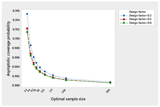
Figure 1. Performance of the asymptotic coverage probability at 90%.

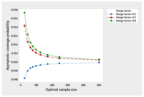
Figure 2. Performance of the asymptotic coverage probability at 95%.

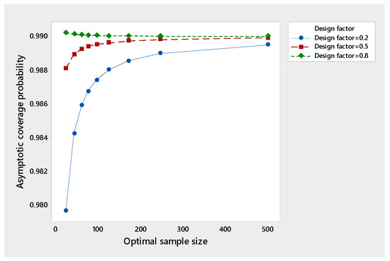
Figure 3. Performance of the asymptotic coverage probability at 99%.

The quantity $\{\frac{a^2\left(\gamma -2\right)+3\left(\gamma +2\right)}{4\gamma }\}$ known as the cost of ignorance (the cost of not knowing the variance ${\sigma }^2$), see Simons [42] for details.

4. The Sensitivity of Three-Stage Sampling to Shift in the Population Inverse Coefficient of Variation

The word sensitivity of sequential procedures means either sensitivity to departure from the underline distribution or sensitivity to shifting in the true parameter value. Bhattacharjee [43], Blumenthal and Govindarajulu [44], Ramkaran [45], Sook and DasGupta [46] were the first who examined the robustness of Stein’s two-stage sampling procedure [47] to departure from normality. Costanza et al. [32] and Son et al. [34], were the first to address the issue of the sensitivity of the three-stage confidence interval against the type II error probability while estimating the mean of the normal distribution. Hamdy [33] studied the same problem for the exponential distribution. However, Hamdy et al. [36] provided a more comprehensive analysis of the departure of both the underline distribution and the shift in the true parameter.

Suppose we need to investigate the capability of the constructed fixed-width confidence interval $I_N$ to signify potential shifts in the true population inverse coefficient of variation ${\theta }_0$ of distance $l\left(\ge 0\right)$ occurring outside the interval when it is incorrectly thought that such shifts never took place. In some applications, like in quality control, it is a matter of concern to closely monitor the sensitivity of the interval to depict any departure from the centerline in order to ensure the creditability of the interval. In this regard, we derive both the null and alternative hypotheses as follows:

$$H_0:\theta ={\theta }_{0}vs.H_a:\theta ={\theta }_1={\theta }_0\pm d\left(l+1\right)\notin I_N\mathrm{for}\mathrm{all}l\ge 0,$$

(18)

where $H_0:\theta ={\theta }_0$, claims that no departure of the true parameter ${\theta }_0$ has taken place, against the alternative hypotheses $H_a$ which alleges that the parameter value differs from ${\theta }_0$ by a distance $1+\ell$ measured in units of the precision $d$.

The probability of not detecting a shift in the true parameter can statistically measure by the corresponding type II error probability ($\beta$-risk), which is, in fact, the conditional probability of not depicting a departure from ${\theta }_0$, when, in fact, the departure actually occurred. In quality assurance ($\beta$-risk), is known as the operating characteristic function

$$\beta (\ell )=P\left({\theta }_0\in I_N|H_a\right)=P\left({\widehat{\theta }}_N-d\le \theta \le {\widehat{\theta }}_N+d|{\theta }_1={\theta }_0\pm \mathrm{d}\left(l+1\right)\right).$$

Since the process has an equal probability of committing a type II error probability above the centerline or below the centerline, we, therefore, consider only the probability of committing a positive shift from the true parameter value ${\theta }_0$.

Let $\tau$ be the probability of committing a type II error probability, which is the probability of no shift occurring given that an actual shift occurred. Our objective is to control the probability of committing a type II error probability. We do so by finding the characteristic operating curve $OC$ that gives the probability of acceptance of various possible values of ${\theta }_1$. The minimum sample size required to control both $\alpha and\tau$ is

$$n^0=\frac{{\left(a+b\right)}^2}{2d^2}{\theta }^2$$

(19)

where $b=Z_{\tau /2}$ is the upper $\tau /2$ point of $N\left(0,1\right)$. For more details, see Nelson [48,49], Hamdy [33], and Son et al. [34].

The second-order approximation of the characteristic operating function under Equations (18) and (19) as $\xi \to \infty$

$$\begin{array}{ll}\beta \left(l\right)& =P\left(\theta \in I_N|H_a\right)={\displaystyle {{\displaystyle \sum }}_{n=m}^{\infty }}P\left(\left|{\widehat{\theta }}_N-{\theta }_1\right|\le d|N=n\right)P\left(N=n\right)\\ & ={\displaystyle {{\displaystyle \sum }}_{n=m}^{\infty }}P\left(-\left(2+l\right)d\le {\widehat{\theta }}_N-{\theta }_0\le -ld\right)P\left(N=n\right)\\ & =E_N\left(\mathsf{\Phi }\left(-ld\sqrt{2N}/\theta \right)\right)-E_N\left(\mathsf{\Phi }\left(-\left(2+l\right)d\sqrt{2N}/\theta \right)\right).\end{array}$$

Utilizing Theorem 3, we obtain

$$E_N\left(\mathsf{\Phi }\left(-ld\sqrt{2N}/\theta \right)\right)=\mathsf{\Phi }\left(-l\left(a+b\right)\right)-\frac{\left(a+b\right)}{8\gamma n^0}\varphi \left(-l\left(a+b\right)\right)l\{{\left(a+b\right)}^2\left(\gamma -2\right)l^2+3\left(\gamma +2\right)\}.$$

Similarly for $E_N\left(\mathsf{\Phi }\left(-\left(2+l\right)d\sqrt{2N}/\theta \right)\right)$.

Hence,

$$\beta \left(l\right)=\mathsf{\Phi }\left(-l\left(a+b\right)\right)-\mathsf{\Phi }\left(-\left(2+l\right)\left(a+b\right)\right)-Q1-Q2+o\left({\xi }^{-2}\right)$$

(20)

where

$$Q1=\frac{\left(a+b\right)}{8\gamma n^0}{\varphi }_{1}l\{{\left(a+b\right)}^2\left(\gamma -2\right)l^2+3\left(\gamma +2\right)\},$$

and

$$Q2=-\frac{\left(a+b\right)}{8\gamma n^0}{\varphi }_2\left(2+l\right)\{{\left(a+b\right)}^2\left(\gamma -2\right){\left(l+2\right)}^2+3\left(\gamma +2\right)\}$$

${\varphi }_1=\varphi \left(-l\left(a+b\right)\right)$ and ${\varphi }_2=\varphi \left(-\left(2+l\right)\left(a+b\right)\right).$

Costanza et al. [32] and Son et al. [34] treated the case of the mean of the normal distribution.

Equation (20) depends on the shift $l,$ the design factor $\gamma ,$ and the optimal sample size $n^0$. Table 2 below shows the $\beta -risk$ values as the shift $k$ increases, and the optimal sample size increases, taking $k=0,0.1,\dots ,1$. As the shift increases, the risk decreases. Figure 4 below demonstrates this idea.

Table 2. The sensitivity of the three-stage procedure as the shift and the optimal sample size increases $\gamma =0.5and\alpha =\tau =5\%.$

Shift	24	43	61	76	96	125	171	246	500
0	0.5000	0.5000	0.5000	0.5000	0.5000	0.5000	0.5000	0.5000	0.5000
0.1	0.3366	0.3414	0.3432	0.3441	0.3448	0.3454	0.3460	0.3465	0.3470
0.2	0.2008	0.2077	0.2103	0.2115	0.2126	0.2135	0.2143	0.2150	0.2158
0.3	0.1065	0.1124	0.1146	0.1156	0.1165	0.1172	0.1179	0.1185	0.1192
0.4	0.0512	0.0544	0.0556	0.0561	0.0566	0.0570	0.0574	0.0577	0.0581
0.5	0.0229	0.0238	0.0242	0.0243	0.0245	0.0246	0.0247	0.0248	0.0249
0.6	0.0098	0.0096	0.0095	0.0095	0.0095	0.0094	0.0094	0.0094	0.0094
0.7	0.0040	0.0036	0.0034	0.0034	0.0033	0.0032	0.0032	0.0031	0.0031
0.8	0.0015	0.0012	0.0011	0.0011	0.0010	0.0010	0.0010	0.0009	0.0009
0.9	0.0005	0.0004	0.0003	0.0003	0.0003	0.0003	0.0003	0.0002	0.0002
1.0	0.0002	0.0001	0.0001	0.0001	0.0001	0.0001	0.0001	0.0001	0.0001

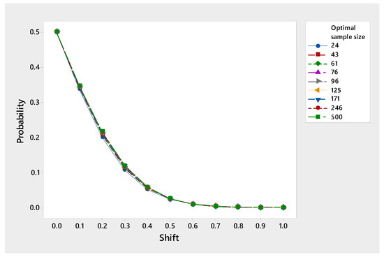
Figure 4. Performance of the characteristic operating curve as the shift increases.

5. The Asymptotic Regret Encountered in Point Estimation of the Inverse Coefficient of Variation

In this section, we aim to find the asymptotic regret that occurs when we use the sample inverse coefficient of variation rather than the population inverse coefficient of variation. We use squared-error loss function with linear sampling cost. A typical situation is in constructing a quality control chart to the inverse coefficient of variation where both estimation of control limits (the upper and the lower control limits) and the centerline are required.

What if we want to utilize the available data to provide a point estimate of $\theta$ (the centerline) under the squared-error loss function with linear sampling cost. Therefore, we assume that the cost incurred in estimating $\theta$ is given by

$$L_n\left(A\right)=A{\left({\widehat{\theta }}_n-\theta \right)}^2+cn,$$

where $c$ is the cost per unit sample. Regarding $A$, the literature in sequential point estimation customarily assumes that $A$ is a known constant, which reflects the cost of estimation and can be permitted to approach $\infty$. However, here, we try to give a better understanding of the nature of $A$ in this context. First, the risk associated with the above loss function is given by

$$R_n\left(A\right)=E{L}_n\left(A\right)=A\frac{{\theta }^2}{2n}+cn.$$

Minimizing the risk associated with the loss function provides the optimal sample size $n^0=\sqrt{\frac{A}{2c}}\theta$. If we have to use the optimal sample size used to construct a fixed $2d$ confidence interval for $\theta$, where the coverage probability is at least the nominal value, to propose ${\widehat{\theta }}_n$ for $\theta$ under the squared error loss function, the constant $A$ should be chosen such that

$$A=\frac{c{a}^4{\theta }^2}{2d^4}=\frac{a^2}{d^2}\left(c{n}^{*}\right).$$

Clearly as $d\to 0,A\to \infty ,$ where

$$A=\left(Fisherinformation,\frac{a^2}{d^2}\right)\times \left(theopimalcostofsamplingc{n}^{*}\right).$$

In this case, the optimal risk is given by $R_{n^{*}}\left(d\right)=2c{n}^{*}$. The asymptotic regret, which is defined as the difference between the risk of using the three-stage procedure minus the optimal risk see, Robbins [38] would be

$$\omega \left(d\right)=R_N\left(d\right)-R_{n^{*}}\left(d\right),$$

where

$$R_N\left(d\right)=AE{\left({\widehat{\theta }}_N-\theta \right)}^2+cE\left(N\right).$$

The risk of the three-stage sampling can be approximated by the upper bound

$$R_N\left(d\right)=c{n}^{*}\left(\gamma +1\right)+c\left(\frac{4+\gamma }{2\gamma }\right).$$

Hence, the asymptotic regret is

$$\omega \left(d\right)=c{n}^{*}\left(\gamma -1\right)+c\left(\frac{4+\gamma }{2\gamma }\right)\mathrm{as}d\to 0.$$

Which provides negative regret. This means that the three-stage procedure does better than the optimal fixed sample size had $\theta$ been known. Martinsek [50] discussed the issue of negative regret in sequential point estimation.

6. Conclusions

This paper theoretically tackles three estimation problems for the population inverse coefficient of variation of the normal distribution under Hall’s three-stage procedure. We obtain asymptotic mathematical forms for the population inverse coefficient of variation, the asymptotic coverage probability, the characteristics operating function, and the asymptotic regret. We find the range of the design factor that makes the three-stage procedure achieve consistency or asymptotic consistency as the width of the interval approaches zero. The asymptotic regret has negative values for all possible values of the design factor.

References

- Nairy, K.S.; Rao, K.A. Tests of Coefficients of Variation of Normal Population. Commun. Stat. Simul. Comput. 2003, 3, 641–661. [Google Scholar] [CrossRef]
- Ahn, K. On the use of coefficient of variation for uncertainty analysis in fault tree analysis. Reliab. Eng. Syst. Saf. 1995, 47, 229–230. [Google Scholar] [CrossRef]
- Gong, J.; Li, Y. Relationship between the Estimated Weibull Modulus and the Coefficient of Variation of the Measured Strength for Ceramics. J. Am. Ceram. Soc. 1999, 82, 449–452. [Google Scholar] [CrossRef]
- Faber, D.S.; Korn, H. Applicability of the coefficient of variation method for analyzing synaptic plasticity. Biophys. J. 1991, 60, 1288–1294. [Google Scholar] [CrossRef]
- Hammer, A.J.; Strachan, J.J.; Black, M.M.; Ibbotson, C.; Elson, R.A. A new method of comparative bone strength measurement. J. Med. Eng. Technol. 1995, 19, 1–5. [Google Scholar] [CrossRef] [PubMed]
- Billings, J.; Zeitel, L.; Lukomnik, J.; Carey, T.S.; Blank, A.E.; Newman, L. Impact of socioeconomic status on hospital use in New York City. Health Aff. 1993, 12, 162–173. [Google Scholar] [CrossRef] [PubMed]
- Brief, R.P.; Owen, J. A Note on earnings risk and the coefficient of variation. J. Financ. 1969, 24, 901–904. [Google Scholar] [CrossRef]
- Pyne, D.B.; Trewin, C.B.; Hopkins, W.G. Progression and variability of competitive performance of Olympic swimmers. J. Sports Sci. 2004, 22, 613–620. [Google Scholar] [CrossRef]
- Kelly, K. Sample size planning for the coefficient of variation from the accuracy in parameter estimation approach. Behav. Res. Methods 2007, 39, 755–766. [Google Scholar] [CrossRef]
- Gulhar, M.; Kibria, B.M.; Albatineh, A.N.; Ahmed, N.U. A Comparison of some confidence intervals for estimating the population coefficient of variation: A simulation study. SORT Stat. Oper. Res. Trans. 2012, 36, 45–68. [Google Scholar]
- McGibney, G.; Smith, M.R. An unbiased signal to noise ratio measure for magnetic resonance images. Med. Phys. 1993, 20, 1077–1079. [Google Scholar] [CrossRef] [PubMed]
- Knight, J.L.; Satchell, S. A Re-Examination of Sharpe’s Ratio for Log-Normal Prices. Appl. Math. Financ. 2005, 12, 87–100. [Google Scholar] [CrossRef]
- Hendricks, W.A.; Robey, K.W. The Sampling Distribution of the Coefficient of Variation. Ann. Math. Stat. 1936, 7, 129–139. [Google Scholar] [CrossRef]
- Koopmans, L.H.; Owen, D.B.; Rosenblatt, J.I. Confidence intervals for the coefficient of variation for the normal and log-normal distribution. Biometrika 1964, 51, 25–32. [Google Scholar] [CrossRef]
- Rao, K.A.; Bhatta, A.R. A note on test for coefficient of variation. Calcutta Stat. Assoc. Bull. 1989, 38, 225–229. [Google Scholar] [CrossRef]
- McKay, A.T. Distribution of the coefficient of variation and the extended t distribution. J. R. Stat. Soc. 1932, 95, 695–698. [Google Scholar] [CrossRef]
- Umphrey, G.J. A comment on McKay’s approximation for the coefficient of variation. Commun. Stat. Simul. Comput. 1983, 12, 629–635. [Google Scholar] [CrossRef]
- Vangel, M.G. Confidence intervals for a normal coefficient of variation. Am. Stat. 1996, 50, 21–26. [Google Scholar]
- Miller, E.G. Asymptotic test statistics for coefficient of variation. Commun. Stat. Theory Methods 1991, 20, 3351–3363. [Google Scholar] [CrossRef]
- Lehmann, E.L. Theory of Point Estimation, 2nd ed.; Wiley: New York, NY, USA, 1983. [Google Scholar]
- Curto, J.D.; Pinto, J.C. The coefficient of variation asymptotic distribution in the case of non-iid random variables. J. Appl. Stat. 2009, 36, 21–32. [Google Scholar] [CrossRef]
- Sharma, K.K.; Krishna, H. Asymptotic sampling distribution of inverse coefficient-of variation and its applications. IEEE Trans. Reliab. 1994, 43, 630–633. [Google Scholar] [CrossRef]
- Albatineh, A.; Kibria, B.M.; Zogheib, B. Asymptotic sampling distribution of inverse coefficient of variation and its applications: Revisited. Int. J. Adv. Stat. Probab. 2014, 2, 15–20. [Google Scholar] [CrossRef]
- Chaturvedi, A.; Rani, U. Fixed-width confidence interval estimation of the inverse coefficient of variation in a normal population. Microelectron. Reliab. 1996, 36, 1305–1308. [Google Scholar] [CrossRef]
- Chow, Y.S.; Robbins, H. On the asymptotic theory of fixed width confidence intervals for the mean. Ann. Math. Stat. 1965, 36, 457–462. [Google Scholar] [CrossRef]
- Chattopadhyay, B.; Kelley, K. Estimation of the Coefficient of Variation with Minimum Risk: A Sequential Method for Minimizing Sampling Error and Study Cost. Multivar. Behav. Res. 2016, 51, 627–648. [Google Scholar] [CrossRef] [PubMed]
- Yousef, A.; Hamdy, H. Three-stage estimation for the mean and variance of the normal distribution with application to inverse coefficient of variation. Mathematics 2019, 7, 831. [Google Scholar] [CrossRef]
- Dantzig, G.B. On the Non-Existence of Tests of Student’s Hypothesis Having Power Function Independent of σ. Ann. Math. Stat. 1940, 11, 186–192. [Google Scholar] [CrossRef]
- Hall, P. Asymptotic Theory and Triple Sampling of Sequential Estimation of a Mean. Ann. Stat. 1981, 9, 1229–1238. [Google Scholar] [CrossRef]
- Hall, P. Sequential Estimation Saving Sampling Operations. J. R. Stat. Soc. 1983, 45, 1229–1238. [Google Scholar] [CrossRef]
- Ghosh, M.; Mukhopadhyay, N.; Sen, P. Sequential Estimation; Wiley: New York, NY, USA, 1997. [Google Scholar]
- Costanza, M.C.; Hamdy, H.I.; Haugh, L.D.; Son, M.S. Type II Error Performance of Triple Sampling Fixed Precision Confidence Intervals for the Normal Mean. Metron 1995, 53, 69–82. [Google Scholar]
- Hamdy, H.I. Performance of Fixed Width Confidence Intervals under Type II Errors: The Exponential Case. South African. J. Stat. 1997, 31, 259–269. [Google Scholar]
- Son, M.S.; Haugh, L.D.; Hamdy, H.I.; Costanza, M.C. Controlling Type II Error while Constructing Triple Sampling Fixed Precision Confidence Intervals for the Normal Mean. Ann. Inst. Stat. Math. 1997, 49, 681–692. [Google Scholar] [CrossRef]
- Yousef, A.; Kimber, A.; Hamdy, H.I. Sensitivity of Normal-Based Triple Sampling Sequential Point Estimation to the Normality Assumption. J. Stat. Plan. Inference 2013, 143, 1606–1618. [Google Scholar] [CrossRef][Green Version]
- Hamdy, H.I.; Son, S.M.; Yousef, S.A. Sensitivity Analysis of Multi-Stage Sampling to Departure of an underlying Distribution from Normality with Computer Simulations. J. Seq. Anal. 2015, 34, 532–558. [Google Scholar] [CrossRef]
- Yousef, A. Construction a Three-Stage Asymptotic Coverage Probability for the Mean Using Edgeworth Second-Order Approximation. In International Conference on Mathematical Sciences and Statistics; Springer: Singapore, 2014; pp. 53–67. [Google Scholar] [CrossRef]
- Yousef, A. A Note on a Three-Stage Sequential Confidence Interval for the Mean When the Underlying Distribution Departs away from Normality. Int. J. Appl. Math. Stat. 2018, 57, 57–69. [Google Scholar]
- Robbins, H. Sequential Estimation of the Mean of a Normal Population. In Probability, and Statistics; Almquist and Wicksell: Uppsala, Sweden, 1959; pp. 235–245. [Google Scholar]
- Anscombe, F.J. Large-sample theory of sequential estimation. In Mathematical Proceedings of the Cambridge Philosophical Society; Cambridge University Press: Cambridge, UK, 1952; Volume 48, pp. 600–607. [Google Scholar]
- Wald, A. Sequential Analysis; Wiley: New York, NY, USA, 1947. [Google Scholar]
- Simons, G. On the cost of not knowing the variance when making a fixed-width interval estimation of the mean. Ann. Math. Stat. 1968, 39, 1946–1952. [Google Scholar] [CrossRef]
- Bhattacharjee, G.P. Effect of non-normality on Stein’s two-sample test. Ann. Math. Stat. 1965, 36, 651–663. [Google Scholar] [CrossRef]
- Blumenthal, S.; Govindarajulu, Z. Robustness of Stein’s two-stage procedure for mixtures of normal populations. J. Am. Stat. Assoc. 1977, 72, 192–196. [Google Scholar] [CrossRef]
- Ramkaran. The robustness of Stein’s two-stage procedure. J. Seq. Anal. 1983, 5, 139–168. [Google Scholar] [CrossRef]
- Oh, H.S.; Dasgupta, A. Robustness of Stein’s two-stage procedure. Seq. Anal. 1995, 14, 321–334. [Google Scholar]
- Stein, C.A. Two-sample test for a linear hypothesis whose power is independent of the variance. Ann. Math. Stat. 1945, 16, 243–258. [Google Scholar] [CrossRef]
- Nelson, L.S. Comments on significant tests and confidence intervals. J. Qual. Technol. 1990, 22, 328–330. [Google Scholar] [CrossRef]
- Nelson, L.S. Sample sizes for confidence intervals with specified length and tolerances. J. Qual. Technol. 1994, 26, 54–63. [Google Scholar] [CrossRef]
- Martinsek, A.T. Negative regret, optimal stopping, and the elimination of outliers. J. Am. Stat. Assoc. 1988, 10, 65–80. [Google Scholar]
© 2019 by the authors. Licensee MDPI, Basel, Switzerland. This article is an open access article distributed under the terms and conditions of the Creative Commons Attribution (CC BY) license (http://creativecommons.org/licenses/by/4.0/).