Immersed Boundary Method Application as a Way to Deal with the Three-Dimensional Sudden Contraction

Abstract

The immersed boundary method has attracted considerable interest in the last few years. The method is a computational cheap alternative to represent the boundaries of a geometrically complex body, while using a cartesian mesh, by adding a force term in the momentum equation. The advantage of this is that bodies of any arbitrary shape can be added without grid restructuring, a procedure which is often time-consuming. Furthermore, multiple bodies may be simulated, and relative motion of those bodies may be accomplished at reasonable computational cost. The numerical platform in development has a parallel distributed-memory implementation to solve the Navier-Stokes equations. The Finite Volume Method is used in the spatial discretization where the diffusive terms are approximated by the central difference method. The temporal discretization is accomplished using the Adams-Bashforth method. Both temporal and spatial discretizations are second-order accurate. The Velocity-pressure coupling is done using the fractional-step method of two steps. The present work applies the immersed boundary method to simulate a Newtonian laminar flow through a three-dimensional sudden contraction. Results are compared to published literature. Flow patterns upstream and downstream of the contraction region are analysed at various Reynolds number in the range $44\le R{e}_D\le 993$ for the large tube and $87\le R{e}_D\le 1956$ for the small tube, considerating a contraction ratio of $\beta =1.97$. Comparison between numerical and experimental velocity profiles has shown good agreement.

1. Introduction

During the last few decades, a lot of effort has been spent by the scientific community working in the field of fluid dynamics, to address two crucial but conflicting key issues in the science of computational fluid dynamics, the need to model increasingly complex boundary conditions and highly accurate results in the least amount of time [1].

The great majority of engineering fluid flow problems are characterized by complex geometries which are often associated with the presence of solid, moving or flexible walls.

The conventional approach to discretize and solve most flows in engineering practice involving complex geometries is not readily fit for Cartesian grids. In complicated geometries, the choice of the grid is not at all trivial. The grid is subject to constraints imposed by the discretization method. In order to be able to deal with complex boundary conditions, whole families of numerical techniques and special methods have been developed. One such method, which is widely used, consists in representing the geometry with body-fitted coordinates. Curvilinear grids, non-orthogonal grids and non-structured grids are three different approaches within this strategy. Also, the grid generation for complex geometries is an issue, consuming a large amount of user time especially when commercial codes are not employed.

Recently, new numerical methodologies have appeared allowing the inclusion of geometrically complex boundary conditions without increasing considerably the computational cost and complexity of the computational grids. One such method is the immersed boundary (IB) method which allows the solution of the differential equations involving complex geometry on simple meshes by introducing forcing conditions on certain surfaces corresponding to the physical location of the complex boundaries. The simulations are then performed on a much simpler domain such as Cartesian meshes [2,3,4,5,6,7,8,9,10]. Mittal and Iaccarino [7] made a good review of the various ways of dealing with IB methods.

Peskin [2,3] reported, at the beginning of the 1970s, simulations of the blood flow in the heart/mitral-valve system assuming a very low Reynolds number and 2D flow. Similar three-dimensional flows that also included the contractile and elastic nature of the boundary were considered successively by Peskin [11] and McQueen and Peskin [12,13]. In Peskin’s formulation, the incompressible Navier-Stokes equations are solved on uniform Cartesian grids and the elastic fibers of the heart walls are immersed in the flow where fluid and fibers exert time varying forces on one another. A Lagrangian coordinate system moving with the local fluid velocity is attached to the fibers and tracks their location in space. The information about the position of the fibers and their forcing on the fluid is transferred to the Eulerian underlying mesh where the flow solution is obtained. In this procedure, the resulting forcing consists of delta functions located on the first cells external to the immersed body which, therefore, cannot be adequately represented on a finite size mesh. For this reason, a smooth transition between the external fluid and internal body cells is introduced which is equivalent to spreading the delta function over a narrow band across the boundary [14]. Since Peskin introduced this method, numerous modifications and refinements have been proposed and several variants of this approach now exist, such as, the Physical Virtual Model [6], the Direct Forcing [8], and more recently, the Multi-direct Forcing [10].

These methods have been used successfully in a variety of flow configurations within finite-difference [6], finite-volume methods [15,16] and Fourier pseudo-spectral [17], to more complex applications involving the simulation of the flow field past a pick-up truck considering a turbulent flow [18]. These methods have produced good results with smaller computational cost than other more conventional methods using non-orthogonal or non-structured grids [14,19]. The immersed boundary method for turbulent flow simulations around complex configurations is illustrated by Iaccario [14]. Sedimentation of hundreds of particles using the immersed boundary method was studied by Wang et al. [10]. Despite the continuous improvement in the immersed boundary methods, the main drawback of these methods is their relatively lack of accuracy near the walls, which is caused by the relatively small number of grid points used to define them [6,20,21]. This issue has been addressed by using a mesh which is locally refined [22].

From a conceptual viewpoint, the immersed boundary method allows the specification of a particular boundary condition in the flow through the addition of a source term to the Navier-Stokes equations. The embedded interface is represented by an arbitrary Lagrangian mesh whereas the flow domain is usually discretised by a Eulerian orthogonal grid. An interpolation function transfers the information from one domain to the other and back. This domain independence allows immersed boundaries to easily displace and/or deform relatively to the fixed grid representing the flow. The way the forcing term is evaluated and the interpolation function is defined, characterizes the different variants of IB formulations.

Fluid flows through a sudden contraction are common in many engineering applications such as piping systems, polymer processes, extrusion, molding and drilling process for oil and gas. This kind of flow is associated with sudden pressure drop and recirculation in the upstream and downstream regions of the contraction plane. The amount of work done in this field in the last 60 years, gives it a place of importance in the fundamental understanding of fluid flow and fluid mechanics in subject configurations. A deep literature review was done by Pienaar [23] on this topic.

Even though the geometry is simple, these entry flows show complex flow patterns [24]. When a fluid flows through a sudden contraction, a stationary flow vortex is present in the corner of the upstream tube and the contraction plane. It reduces the available flow area and the fluid accelerates and results in a partially developed velocity profile at the entrance of the downstream tube. In turbulent flow there is a marked drop in pressure as the fluid passes through the contraction. The pressure loss is due to an increase in velocity and the loss of energy in turbulence. There is a rise in pressure at the upstream corner of the contraction due to streamline curvature so that the centrifugal action causes the pressure at the pipe wall to be greater than in the center of the stream. The streamlines continue to curve downstream of the contraction to form a cross section where a minimum pressure and maximum velocity are obtained. This region is known as the vena contracta. The contracted flowing stream is surrounded by fluid that is in a state of turbulence but has very little forward motion. Downstream of the vena contracta the flow stream expands, the velocity decreases and the pressure rises [23]. Associated with these changes in pressure loss are increased erosion rates as well as increased heat and mass transfer rates in the regions where separated flow occurs.

Flow in pipes with sudden contraction in cross sectional area has been extensively studied. A large number of publications provide some experimental data on integral flow properties such as wall pressure drop, flow redevelopment length after the contraction, and general information on the mean flow pattern obtained mostly from flow visualization studies. The development of experimental non-intrusive techniques has allowed to obtain information about the kinematic of fluid flow, like velocity profiles, turbulence intensities, and other important variables.

Durst et al. [25] conducted a numerical and experimental study of laminar flow in a pipe with a sudden contraction of $\beta =1.87$. The numerical approach was performed by solving the governing two-dimensional, elliptic, partial differential equation by the finite-difference scheme. The flow was considered to be axisymmetric and stationary and the grid distribution in the calculation domain was non-uniform in both the longitudinal and radial coordinate directions. The experimental investigations were carried out through the Laser Doppler Anemometry (LDA) measurements. Tests allowed to obtain velocity profiles along the upstream and downstream regions of the contraction plane. The numerical tests provided information about the vortex region, including the length of flow separation in the concave and convex corners of the plane of contraction. Comparison between numerical and experimental results yielded good agreements for most of flow field.

Sanchez [26] investigated experimentally the Newtonian laminar flow through an axisymmetric sudden contraction with $\beta =1.97$. The experimental measurements are carried out with the Particle Image Velocimetry technique (PIV-2D) to obtain the two-dimensional velocity field along the upstream region for $R{e}_D=185$, 365, 568, 993 and 1266. Velocity profiles in the longitudinal and radial directions along the upstream flow region of the contraction and flow pattern along the upstream region were studied.

The goal of the present work is to apply IB method to simulate a Newtonian, incompressible and laminar flow through a sudden contraction solving the governing three-dimensional, partial differential equation in Cartesian meshes. The geometry of the present problem is simple, however the entry flow shows complex flow patterns. Structured meshes are being used to show that the IB method is an interesting alternative to deal with the sudden contraction case.

2. Numerical Investigations

2.1. Mathematical Model

The equations of mass and momentum conservation (also known as the Navier-Stokes equations) are used to model the cases simulated in this present work, considering an incompressible flow in a Newtonian fluid. In Cartesian form, the continuity equation is given by,

$$\frac{\partial u_j}{\partial x_j}=0$$

(1)

while the momentum equation in the ‘i’ direction is given by,

$$\frac{\partial u_i}{\partial t}+\frac{\partial \left(u_i{u}_j\right)}{\partial x_j}=-\frac{1}{\rho }\frac{\partial p}{\partial x_i}+\frac{\partial }{\partial x_j}\left[\nu \left(\frac{\partial u_i}{\partial x_j}+\frac{\partial u_j}{\partial x_i}\right)\right]+\frac{f_i}{\rho }$$

(2)

where $x_i$ is the i-th component of the position vector x, $u_i$ is the i-th component of the velocity vector u, p is the pressure, $\rho$ and $\nu$ are the density and the kinematic viscosity of the fluid and $f_i$ is the i-th component of the force vector f which represent any external force acting on the fluid.

The immersed boundary method allows the specification of a particular boundary condition in the flow through the addition of a source term $f_i$ in the momentum equations (Equation (2)). This source term is calculated in the Lagrangian domain and transmitted to the Eulerian domain to account for the presence of the boundary walls (geometry). The term $f_i$ is null in all Eulerian grid, except in volumes neighbor to the Lagrangian markers. Mathematically the source term can be represent as:

$$\overrightarrow{f}(\overrightarrow{x},t)={\int }_{\mathsf{\Gamma }}\overrightarrow{F}({\overrightarrow{x}}_k,t)\delta (\overrightarrow{x}-{\overrightarrow{x}}_k)d{\overrightarrow{x}}_k$$

(3)

where $\delta \left(x\right)$ is the auxiliary Dirac delta function, k denotes a Lagrangian variable and $\overrightarrow{F}({\overrightarrow{x}}_k,t)$ is the Lagrangian force, which is determined in the points of the object interface.

2.2. Numerical Methods

The governing equations (Equations (1) and (2)) are discretized by the finite volume method, where the advective-diffusive terms are discretized using the central differencing scheme, in a staggered arrangement, as proposed by Patankar [27]. In a simple rectilinear mesh discretization, the components u, v and w are positioned in the volume’s normal faces in x, y and z directions, respectively whereas scalar values, such as pressure, are located at the volume center [28]. The pressure and velocity are coupled using the explicit fractional time-step (second order accuracy) Adams-Bashforth method [29]. Thus, first the velocity field is estimated as ${\mathit{u}}^{*}$, in Equation (4).

$$\frac{{\mathit{u}}^{*}-{\mathit{u}}^t}{\mathsf{\Delta }t}=\frac{3}{2}{A}^t-\frac{1}{2}{A}^{t-1}-\frac{1}{\rho }\nabla p^t$$

(4)

where t is the time instant and A contains the advective and diffusive terms. The velocity $u^{t+1}$ is estimated using:

$$\frac{{\mathit{u}}^{t+1}-{\mathit{u}}^{*}}{\mathsf{\Delta }t}=-\frac{1}{\rho }\nabla p^{\prime }$$

(5)

where the pressure fluctuation $p^{\prime }$ is determined by the solution of a Poisson equation in the form of,

$${\nabla }^2{p}^{\prime }=\frac{\rho }{\mathsf{\Delta }t}\nabla ·{\mathit{u}}^{*}$$

(6)

leading to the pressure $p^{t+1}$ estimation through,

$$p^{t+1}=p^t+p^{\prime }$$

(7)

Computational Aspects

It’s worth mentioning the solution of Equation (6) is performed by the packages Epetra, AztecOO and ML of framework Trilinos, which provides a free general implementation of scientific computational tools in parallel, as libraries for linear algebra and solvers [30]. The method Generalized Minimum Residual (GMRES) was used as predefined parameter for the AztecOO library, preconditioned through the algebraic multigrid method (AMG), in the ML library [31]. To ensure load balancing, the library Zoltan was employed and between the algorithms available for the load balancing, the recursive coordinate bisection (RCB) was selected, since this method has shown low computational cost [32].

2.3. Immersed Boundary Method

The method Direct Forcing (MDF) was proposed by Uhlmann [8]. Other authors developed variations of this method [10,33,34]. A force $\overrightarrow{F}({\overrightarrow{x}}_k,t)$ based on MDF method is imposed on the Lagrangian markers to modify its velocity to be equal to the desired velocity $u_{IBM}$ at the immersed boundary.

From Equation (2),

$$\frac{f_i}{\rho }=\frac{\partial u_i}{\partial t}+\frac{\partial \left(u_j{u}_i\right)}{\partial x_j}+\frac{1}{\rho }\frac{\partial p}{\partial x_i}-\frac{\partial }{\partial x_j}\left[\nu \left(\frac{\partial u_i}{\partial x_j}+\frac{\partial u_j}{\partial x_i}\right)\right]$$

(8)

and,

$$\frac{F_{ki}}{\rho }=\frac{\partial u_{ki}}{\partial t}+\frac{\partial \left(u_{kj}{u}_{ki}\right)}{\partial x_{kj}}+\frac{1}{\rho }\frac{\partial p}{\partial x_{ki}}-\frac{\partial }{\partial x_{kj}}\left[\nu \left(\frac{\partial u_{ki}}{\partial x_{kj}}+\frac{\partial u_{kj}}{\partial x_{ki}}\right)\right]$$

(9)

where the index k denotes a Lagrangian variable and $F_{ki}(x_k,t)$ represents the Lagrangian force. Applying the Euler temporal discretization from Equation (9), it becomes:

$$\frac{F_{ki}}{\rho }=\frac{u_{ki}^{t+\mathsf{\Delta }t}-u_{ki}^t}{\mathsf{\Delta }t}+RH{S}_{ki}^t$$

(10)

where $\mathsf{\Delta }t$ is the discrete interval and $RHS$ is a composed by the advective, diffusive and pressure terms:

$$RH{S}_{ki}^t=\frac{\partial \left(u_{kj}{u}_{ki}\right)}{\partial x_{kj}}+\frac{1}{\rho }\frac{\partial p}{\partial x_{ki}}-\frac{\partial }{\partial x_{kj}}\left[\nu \left(\frac{\partial u_{ki}}{\partial x_{kj}}+\frac{\partial u_{kj}}{\partial x_{ki}}\right)\right]$$

(11)

Adding a temporal parameter, $u_{ki}^{*}$, Equation (10) can be rewritten as,

$$\frac{F_{ki}}{\rho }=\frac{u_{ki}^{t+\mathsf{\Delta }t}+u_{ki}^{*}-u_{ki}^{*}-u_{ki}^t}{\mathsf{\Delta }t}+RH{S}_{ki}^t$$

(12)

Equation (12) can be decomposed into two complementary equations:

$$\frac{u_{ki}^{*}-u_{ki}^t}{\mathsf{\Delta }t}+RH{S}_{ki}^t=0$$

(13)

and,

$$\frac{F_{ki}}{\rho }=\frac{u_{ki}^{t+\mathsf{\Delta }t}-u_{ki}^{*}}{\mathsf{\Delta }t}=\frac{u_{iIBM}-u_{ki}^{*}}{\mathsf{\Delta }t}$$

(14)

where $u_{iIBM}$ is the immersed boundary velocity. Under the effect of the Immersed Boundary force, the velocity on the Lagrangian marker $x_k$ at time $t+\mathsf{\Delta }t$$u_{ki}^{t+\mathsf{\Delta }t}$ can be modified to the desired velocity $u_{iIBM}$ [10]. $u_{ki}^{*}$ is calculated using Equation (15). This variable is calculated using the moving-least-squares reconstruction method (MLS) [35]. This method is employed to enforce the proper boundary condition on all the Eulerian grid nodes influenced by the immersed body. First, it computes the force function on the Lagrangian markers and then transfers this function to the Eulerian grid nodes. In this work, the transfer operators were constructed using MLS shape functions with compact support [36].

Using the MLS, $u_{ki}^{*}$ for each Lagrangian marker can be approximated in its support domain as follows:

$$u_{ki}^{*}\left({\mathit{x}}_k\right)=\sum _{j=1}^m{p}_j\left({\mathit{x}}_k\right)a_j\left({\mathit{x}}_k\right)={\mathit{p}}^T\left({\mathit{x}}_k\right)\mathit{a}\left({\mathit{x}}_k\right)$$

(15)

where $\mathit{p}\left({\mathit{x}}_k\right)$ is the basis functions vector of length m, $\mathit{a}\left({\mathit{x}}_k\right)$ is a vector of coefficients and ${\mathit{x}}_k$ is the position of the Lagrangian marker. Adopting a linear basis, ${\mathit{p}}^T\left({\mathit{x}}_k\right)$ is an efficient choice and would represents the field variation for all variables up to the accuracy of the spatial discretization scheme employed.

$${\mathit{p}}^T\left({\mathit{x}}_k\right)=\left[1x_k{y}_k{z}_k\right]$$

(16)

To obtain the coefficient vector, $a_j\left({\mathit{x}}_k\right)$ from the basis functions Equation (16), the following weighted L2-norm is defined:

$$J=\sum _{k=1}^{np}W({\mathit{x}}_k-\mathit{x}){\left[{\mathit{p}}^T\left(\mathit{x}\right)\mathit{a}\left({\mathit{x}}_k\right)-u_i^{*}\right]}^2$$

(17)

where $\mathit{x}$ is the position vector of the Eulerian node, $W({\mathit{x}}_k-\mathit{x})$ is a given weight function, $np$ is the total number of grid points in the interpolation scheme and $u_i$ is the i-th component of the velocity vector u in the Eulerian domain. Minimizing J with respect to $\mathit{a}\left(\mathit{x}\right)$ leads to the following set of equations:

$$\begin{array}{c}\mathit{A}\left({\mathit{x}}_k\right)\mathit{a}\left({\mathit{x}}_k\right)=\mathit{B}\left({\mathit{x}}_k\right){\mathit{u}}_i^{*}\\ \mathit{A}\left({\mathit{x}}_k\right)=\sum _{k=1}^{np}W({\mathit{x}}_k-\mathit{x})\mathit{p}\left(\mathit{x}\right){\mathit{p}}^T\left(\mathit{x}\right)\\ \mathit{B}\left({\mathit{x}}_k\right)=[W(\mathit{x}-{\mathit{x}}^1)\mathit{p}\left({\mathit{x}}^1\right)\dots W(\mathit{x}-{\mathit{x}}^{np})\mathit{p}\left({\mathit{x}}^{np}\right)]\end{array}$$

(18)

The size of matrix $\mathit{A}\left({\mathit{x}}_k\right)$ and $\mathit{B}$ depend on the size of the basis vector, which is $4\times 4$ and $4\times np$, respectively for the present study. Assuming the matrix $\mathit{A}$ is not singular, we have:

$$\mathit{a}\left({\mathit{x}}_k\right)={\mathit{A}}^{-1}\left({\mathit{x}}_k\right)\mathit{B}\left({\mathit{x}}_k\right){\mathit{u}}_i^{*}$$

(19)

Combining Equations (15) and (19) leads to,

$$u_{ki}^{*}\left({\mathit{x}}_k\right)=\sum _{k=1}^{np}\varphi \left(\mathit{x}\right)u_i^{*}={\mathit{\varphi }}^T\left(\mathit{x}\right){\mathit{u}}_i$$

(20)

where $\mathbf{\Phi }\left(\mathit{x}\right)=\mathit{p}\left({\mathit{x}}_k\right)\left[{\mathit{A}}^{-1}\left({\mathit{x}}_k\right)\mathit{B}\left({\mathit{x}}_k\right)\right]$ is a column vector with length $np$, containing the shape function values. Cubic splines are used for the weight function, $W({\mathit{x}}_k-\mathit{x})$, which can be written as:

$$\begin{array}{cc}\hfill W({\mathit{x}}_k-\mathit{x})& =\left\{\begin{array}{cc}2/3-4{\overline{r}}_k^2+4{\overline{r}}_k^3,\hfill & \mathrm{if} {\overline{r}}_k\le 0,5\hfill \\ 4/3-4{\overline{r}}_k+4{\overline{r}}_k^2-4/3{\overline{r}}_k^3,\hfill & \mathrm{if} 0,5\ge {\overline{r}}_k\le 1\hfill \\ 0,\hfill & \mathrm{if} {\overline{r}}_k>1\hfill \end{array}\right.\end{array}$$

where ${\overline{r}}_I=|{\mathit{x}}_k-\mathit{x}|/H_i$ and $H_i$ is a half length of a rectangular box centered at the location of the marker. These functions are monotonically decreasing and are sufficiently smooth in the support domain. The resulting shape functions reproduce exactly the linear polynomial contained in their basis and possess the partition of unity property ${\displaystyle \sum _{k=1}^{np}}\varphi \left(\mathit{x}\right)=1$. Also, the field approximation is continuous on the global domain as the MLS shape functions are compatible.

$u_{ki}^{*}$ is calculated using Equation (20) which is then substituted into Equation (14) to obtain the volume force $F_{ki}$. To transfer this force to the Eulerian domain associated with each marker, the same shape functions used in the interpolation procedure can be used if properly scaled by a factor $e_f$. The final forces on the Eulerian grid can be written as:

$$f_i=\sum _{k=1}^{nk}{e}_{fk}\varphi F_{ki}$$

(21)

where $f_i$ is the volume force in the Eulerian domain due to the contribution of the $nk$ Lagrangian markers. To properly rescale the shape functions it is required that the total force acting on the fluid is not changed by the transfer:

$$\sum _{I=1}^n{f}_i\mathsf{\Delta }V=\sum _{k=1}^{nk}{F}_{ki}\mathsf{\Delta }{V}_k$$

(22)

where $\mathsf{\Delta }V=(dx·dy·dz)$ is the volume associated with the Eulerian grid point and $V_k=A_k·h_k$ is the volume associated with the Lagrangian maker, with $h_k=\frac{1}{3}{\displaystyle \sum _{I=1}^n}{\varphi }_I(dx·dy·dz)$. The total number of forced grid points and the total of Lagrangian markers are n and $nk$ respectively.

From the average Eulerian grid volume associated with the Lagrangian marker $\overline{V}$, the scaling factor $e_{fk}$ is defined as:

$$e_{fk}=\frac{V_k}{\overline{V}}$$

(23)

Using the Eulerian forcing function from Equation (21) it is possible to update the estimated velocity from the Adams-Bashforth equation (Equation (4)) in order to insert the boundary conditions on the immersed body. Thus the new estimated velocity field can be written as:

$$u_i^{*}=u_i^{*}+f_i\mathsf{\Delta }t$$

(24)

The resulting approximate velocity field, $u_i^{*}$, which is not divergence-free, can be projected into a divergence-free space by applying a correction of the form as showed in Equation (5).

3. Problem Description

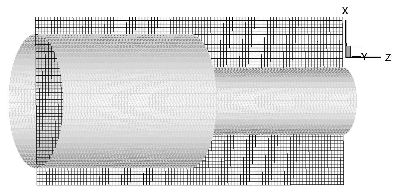
The problem consists in a numerically investigation of an Newtonian laminar flow in a three-dimensional sudden contraction. Fluid flow through a sudden contraction is shown in Figure 1. The Cartesian coordinates system (x,y,z) is adopted for the Eulerian domain. To minimize the Eulerian domain size which is $0.25\times 0.25\times 0.7$ m in x, y and z direction respectively, a parabolic inlet profile was implemented [37] showing a fully developed behaviour in the upstream region with a bulk velocity $U_1$. The upstream pipe has an inner diameter of $D=0.239$ m and a length of $L_D=0.4$ m, and the downstream section is a pipe with a diameter $d=0.1215$ m and a length of $L_d=0.3$ m with a bulk velocity $U_2$. Important parameters related to the study of fluid flow through a contraction are: the contraction ratio, $\beta =D/d$ and the upstream Reynolds number, $R{e}_D=\rho U_{1}D/\nu$. The contraction ratio adopted in this present work is $\beta =1.97$ [26]. The density of the fluid $\rho =1.0$ kg/m${}^3$ and the kinematic viscosity was varied to set the Reynolds number.

The boundary conditions applied for the computations were as follows:

$$\begin{array}{c}\hfill Inlet:u=U_{max}\left[1-{\left(\frac{r}{R_D}\right)}^2\right]\\ \hfill Oulet:\frac{\partial u}{\partial z}=\frac{\partial v}{\partial z}=\frac{\partial w}{\partial z}=0\\ \hfill walls:u=v=w=0\end{array}$$

Based on mass conservation, in control volume form, the relation between the velocity and the Reynold number upstream and downstream are defined as:

$$U_2=U_1{\beta }^2$$

(25)

$$R{e}_d=R{e}_D\beta$$

(26)

The Lagrangian markers which represent the sudden contraction surface are imported from any mesh generation software which returns waveform object format. Figure 2 shows the Lagrangian markers which represent the three-dimensional surface of the sudden contraction associated with a Eulerian plane.

4. Results and Discussion

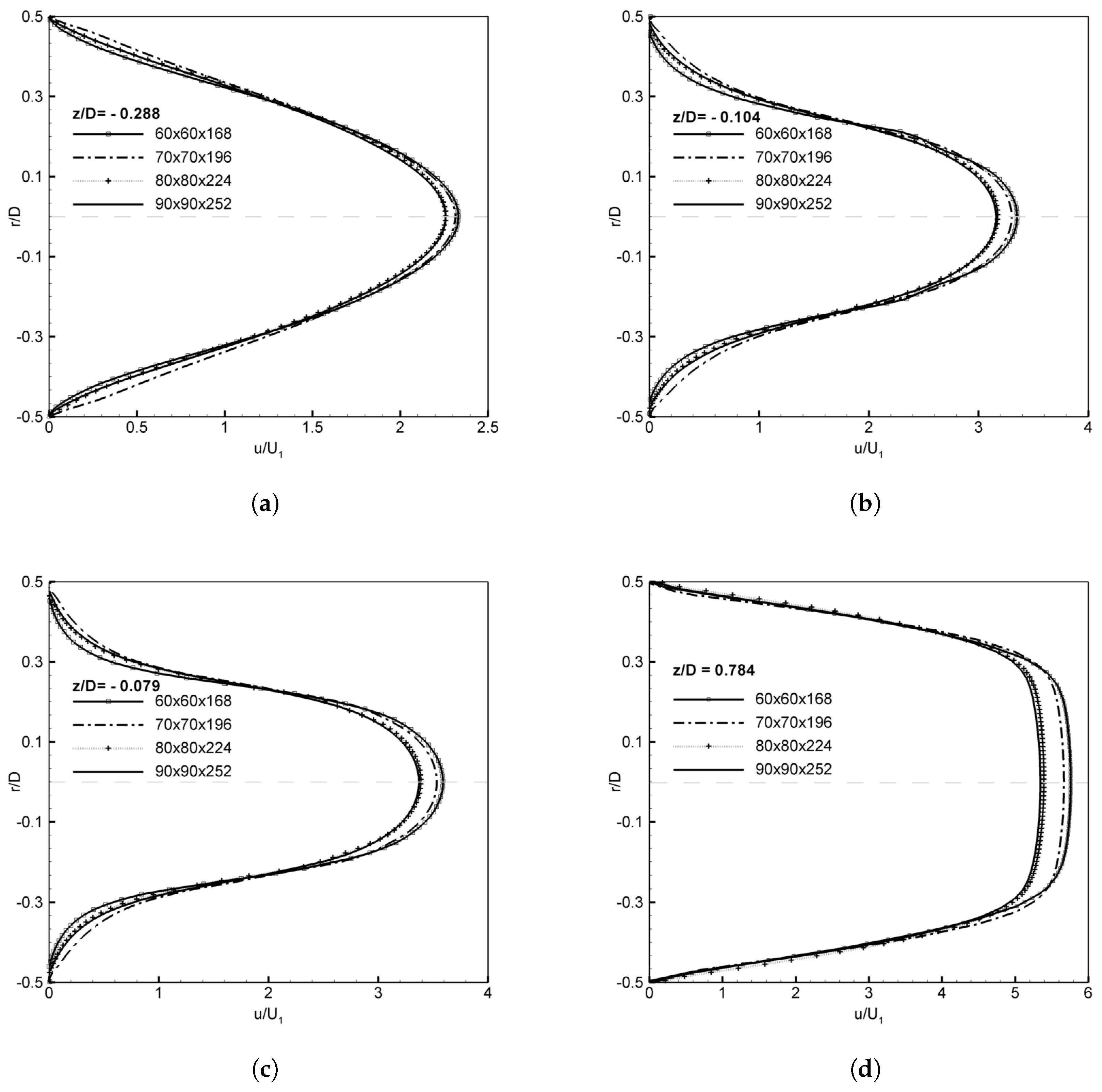
In this work, flow patterns upstream and downstream of the contraction region are analysed at various Reynolds number in the range $44\le R{e}_D\le 993$ for the large tube and $87\le R{e}_D\le 1956$ for the small tube. Grid independence was judged by comparing the results with other works [25,26]. It was found that a grid density of $90\times 90\times 252$ is sufficient to provide a profile in the contraction that is independent of the grid density, as shown in the Appendix A.

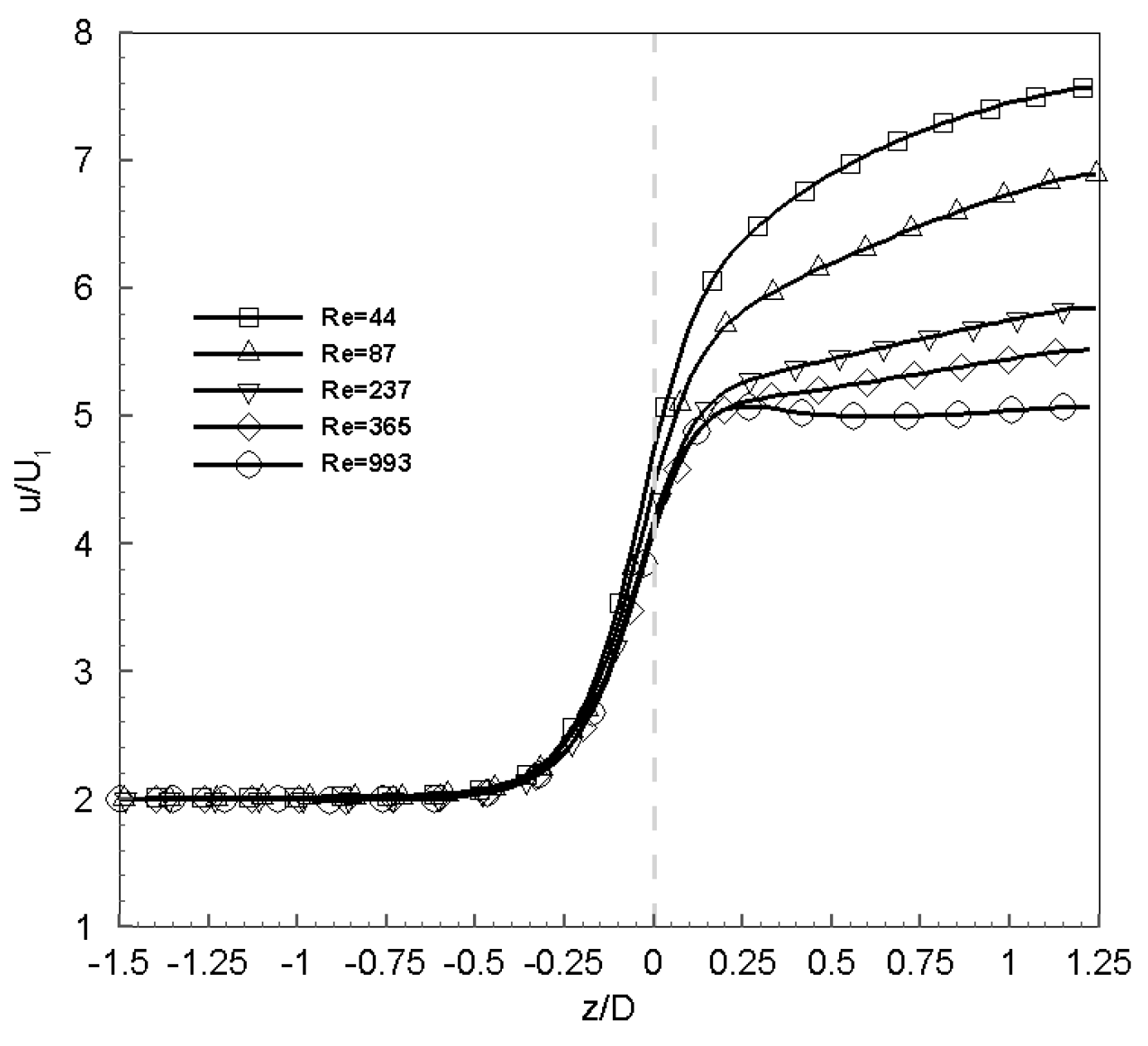
A stationary flow vortex is present in the corner of the upstream tube just before the contraction plane. This reduces the available flow area forcing the fluid to accelerate which results in a partially developed velocity profile at the entrance of the downstream tube. The upstream influence of sudden contraction is limited to a region smaller than 0.6D. This is in agreement with the work by Sanchez [26]. As shown in Figure 3, the downstream pipe length was not long enough to ensure the velocity redevelops into a parabolic profile.

The velocity profile at the inlet of the downstream pipe changes with Reynolds number. This velocity profile shows velocity maxima close to the pipe walls (velocity overshoot) and a flat distribution of velocity in the center part of the pipe. Despite this occurrence, there is a redevelopment of the profile until reaching the fully developed parabolic distributions. The velocity overshoot is associated with strong, axial positive pressure gradients and the resultant separation region which occur locally in the near wall region of the smaller pipe and just downstream of the plane of contraction [25]. The depth of the concavity increases with $Re$ and $1/\beta$ [23]. Durst et al. [25] reported that both the experiments and computations show these velocity overshoots for Reynolds number $R{e}_D\ge 125$ and $\beta =1.87$. As shown in Figure 4, for the present contraction ratio, $\beta =1.97$, these velocity overshoots are present when $R{e}_D\ge 87$. The effect of the concavity is the reason the axial velocity at center line decreases as Reynolds number increases, as seen in Figure 3.

Durst et al. [25] stated that the velocity overshoot does not exist in the plane of contraction but develops immediately downstream of it; however, the present results show velocity overshoot profiles at the contraction plane and immediately downstream of it, as well.

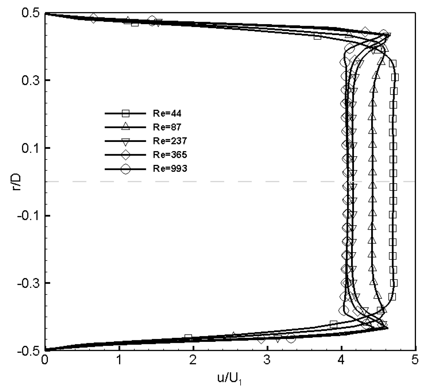
The streamlines continue to curve downstream of the contraction to form a cross section where a minimum pressure and maximum velocity are obtained. This region is known as the vena contracta. The contracted flowing stream is surrounded by fluid that has very little forward motion. Downstream of the vena contracta the flow stream expands, the velocity decreases and the pressure rises [23]. Associated with these changes in pressure are increased erosion rates as well as increased heat and mass transfer rates in the regions where flow separation occurs. From the range of Reynolds numbers simulated, the presence of the vena contracta was notice at $R{e}_D=993$, where a maximum velocity and minimum pressure are obtained downstream of the contraction at the position $z/D\approx 0.25$ (Figure 3 and Figure 5a), respectively. Expanded views on the pressure field at $R{e}_D=993$, associated with streamlines were also used to visualize the presence of the vena contracta, which is shown in Figure 5e. Durst et al. [25] found the existence of the vena contracta for $R{e}_D\ge 300$ when $\beta =1.87$. Based on other works [38,39] it is possible to conclude that as the contraction ratio increases, the Reynolds number to obtain the vena contracta increases as well. Regarding the pressure losses caused by the sudden contraction, for the Reynolds numbers studied the results are given in Figure 5b. This figure also reproduces data by Astarita and Greco [40], Sylvester and Rosen [38], Durst et al. [25] and Sanchez [26]. There are the same tendency of all works, as Reynolds number increases, the dimensionless pressure loss decreases. The pressure fields at $Re=365$ and 993 are shown in Figure 5c,d, respectively.

Where $\mathsf{\Delta }{p}_{con}$ is obtained through the pressure gradient extrapolation of fully developed flow in the downstream and upstream region of the contraction plane [41] and the dimensionless pressure loss is defined as

$$\mathsf{\Delta }{p}_{con}^{*}=\frac{\mathsf{\Delta }{p}_{con}}{\rho U_2^2/2}$$

(27)

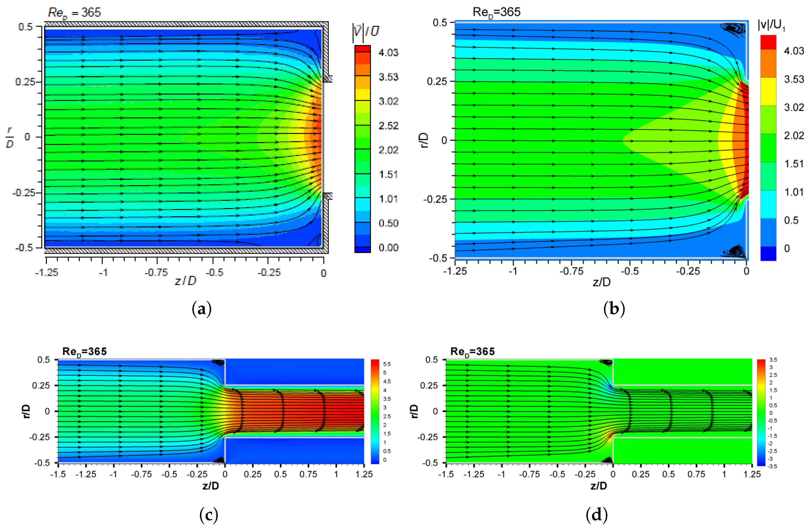
The upstream region obtained from Sanchez [26] (Figure 6a) is compared to the present result in the same region at $R{e}_D=365$ (Figure 6b) for the velocity magnitude $\overrightarrow{V}/U_1$, adimensionalized with the upstream bulk velocity $U_1$, on a plane containing the centerline. There is a good agreement between the studies, although the experimental work from Sanchez [26] was not able to capture the stationary vortex in the upstream region by the streamlines, due to the low velocity tracer particles used in PIV technique which tend to adhere to the pipe, a common problem in regions of vortex formation.

Figure 6c,d show the axial and radial velocity contour plot and streamlines on a plane containing the centreline at $R{e}_D=365$ and steady state conditions for both regions, upstream and downstream. It is possible to visualize the presence of the stationary vortex (separation region) in the upstream region just before the contraction. Streamlines are smooth throughout the domain due to the laminar nature of the flow field.

The radial velocity is imposed null at the domain entrance and show only large values in the immediate vicinity of the plane of contraction in its corners.

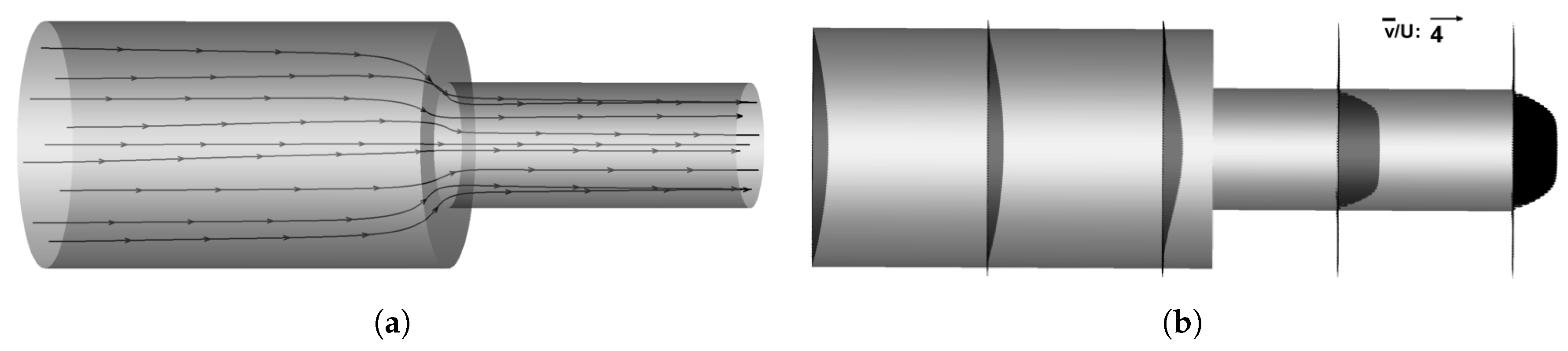
Flow pattern through the streamlines and the velocity vector for some planes are shown in Figure 7 (three-dimensional domain). In both figures it is possible to visualise the flow adaptation to pass through the sudden contraction, first, in the entrance of the domain the flow has a parabolic profile, then under influence of sudden contraction (smaller than 0.6) the flow adapt to pass through the sudden contraction, where the profile becomes thinner having higher velocity in the center region and lower velocity close to the wall. In the downstream region, the profile is adapting to achieve fully developed velocity profile showing higher velocity when compared to the upstream region due to smaller diameter.

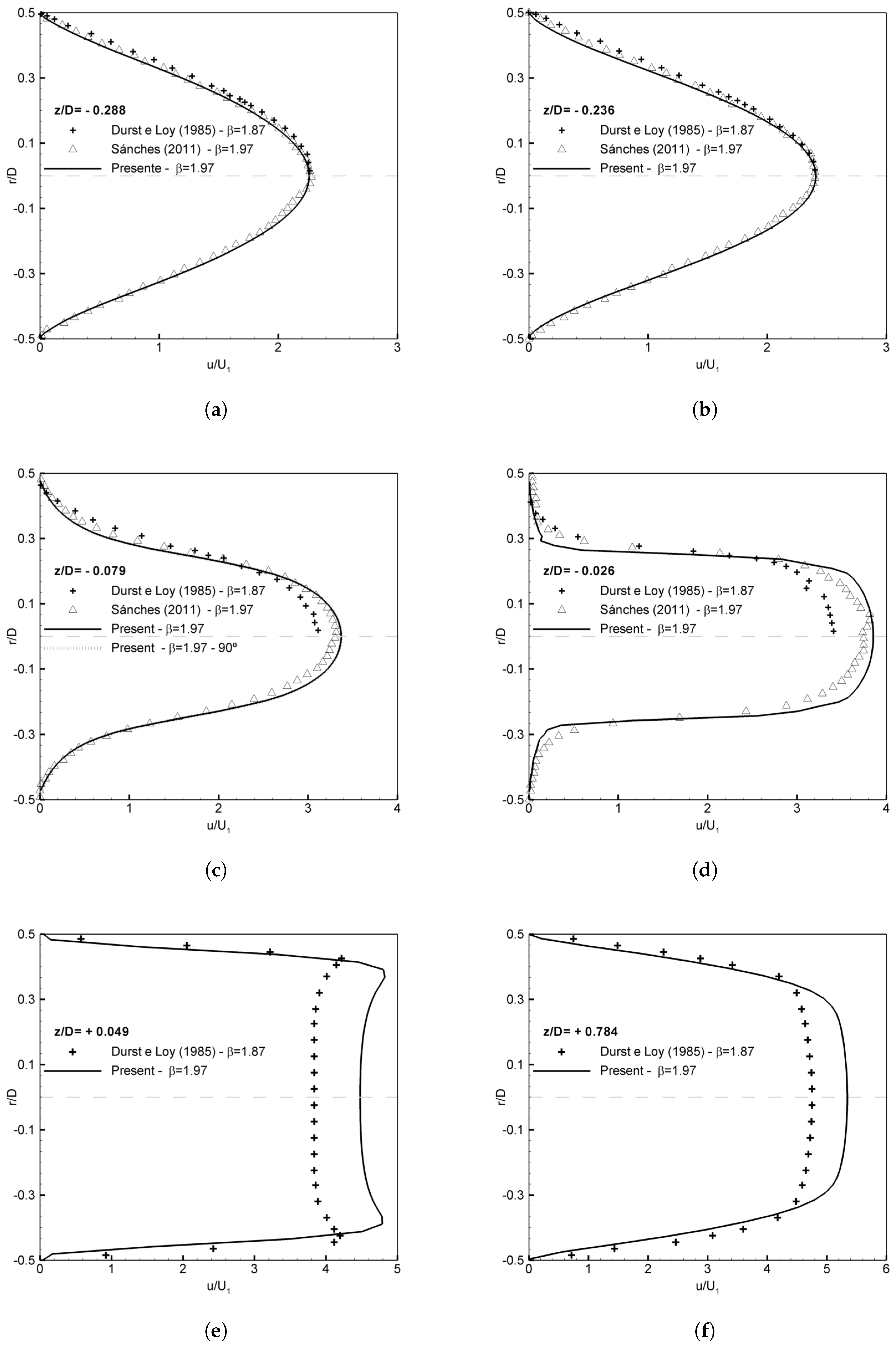
Figure 8 compares velocity profiles upstream and downstream of the contraction with other published literature. Durst et al. [25] conducted an experimental study of laminar flow in a pipe with a sudden contraction of $\beta =1.87$ and $R{e}_D=372$ (slightly different Reynolds number from this work). The experimental investigations were carried out using LDA techniques in both regions, upstream and downstream. Sanchez [26] investigated flow along the upstream flow region of a sudden contraction having $\beta =1.97$ and $R{e}_D=365$ through experimental techniques using PIV-2D methods.

Even though the positions $z/D=-0.288$ and $z/D=-0.236$ are under the influence of the sudden contraction, this influence is quite weak, having a good agreement between the present result and the reference works (Figure 8a,b). Nearer to the sudden contraction, the influence increases, as shown at the position $z/D=-0.079$ (Figure 8c), where there is a good agreement between the cases where the contraction ratio and Reynolds number have the same values [26] and the same tendency with the Durst et al. [25] which has lower contraction ratio and slightly different Reynolds number. The difference results between the present work and Durst et al. [25] relies on the contraction ratio and Reynolds number difference, once the present work has a higher contraction ratio it is expected higher velocity (Equation (26)).

To ensure axisymmetry a second profile on a line located ninety degree from the original one is also plotted in Figure 8c. This shows an identical result, implying axisymmetric behavior.

Figure 8d present a profile near to the sudden contraction ($z/D=-0.0026)$, showing agreement between the results of the present paper and Sanchez [26], although there is a slight difference between the axial velocity profiles. Durst et al. [25] has shown the same tendency, as well. Once in the downstream region the only reference is Durst et al. [25], it is possible to visualize the same tendency for both position, $z/D=0.049$ (Figure 8e) and $z/D=0.784$ (Figure 8f). In the first position the presence of the velocity overshoot is clearly observed and for the second position, a redevelopment of the profile to reach the fully developed parabolic distributions is observed.

The percentage error of the maximum dimensionless axial velocity between the present results and Sanchez [26] at $R{e}_D=365$ and $\beta =1.97$ presented in

Table 1. Percentage error in maximum velocity at $R{e}_D=365$ and $\beta =1.97$ for some positions ($z/D$).

$\mathit{z}/\mathit{D}$	$\mathit{u}/\mathit{U}$
	Present	Sanchez [26]	Error (%)
$-0.288$	$2.26$	$2.28$	$0.88$
$-0.236$	$2.41$	$2.40$	$0.26$
$-0.079$	$3.37$	$3.31$	$1.70$
$-0.026$	$3.85$	$3.81$	$1.08$

, has maximum error within $1.7$%. Experimental uncertainty analysis was not performed by Sanchez [26] to compare this error, properly.

Where the percentage error is defined as

$$error(\%)=|\frac{{(u/U)}_{NUM}-{(u/U)}_{EXP}}{{(u/U)}_{NUM}}|\times 100$$

(28)

5. Conclusions

In this paper, Newtonian laminar flow through a three-dimensional sudden contraction, having a contraction ratio of $\beta =1.97$, was numerically investigated using the immersed-boundary (IB) method. A structured grid in Cartesian coordinate was employed for the Eulerian domain and the sudden contraction surface was represented by the Lagrangian markers. The numerical implementation of Cartesian coordinates is simpler than the body-fitted coordinates. The IB method was able to represent the sudden contraction well, compared to other published literature. The present results show:

The upstream influence of sudden contraction is limited to a region smaller than 0.6D.

For Reynolds number in excess of $R{e}_D\ge 87$ the profiles of the axial velocity component show a characteristic velocity overshoot.

From the range of Reynolds numbers simulated, the presence of the vena contracta was notice at $R{e}_D=993$, where a minimum pressure and maximum velocity are obtained downstream of the contraction. Preliminary tests confirm it remains for higher Reynolds number.

Regarding the pressure losses caused by the sudden contraction, as Reynolds number increases, the dimensionless pressure loss decreases.

There was good agreement when comparing the profiles from the current simulation with published experimental data, showing the IB method is an interesting alternative to deal with the sudden contraction.