Article

Multiscale CT-Based Computational Modeling of Alveolar Gas Exchange during Artificial Lung Ventilation, Cluster (Biot) and Periodic (Cheyne-Stokes) Breathings and Bronchial Asthma Attack

1
Moscow Institute of Physics and Technology (State University), 9 Instituskii Lane, 141701 Dolgoprudny, Russia
2
Institute of Computer-Aided Design, RAS, 19/18 2nd Brestskaya St., 123056 Moscow, Russia
3
Institute of Numerical Mathematics, RAS, 8 Gubkina St., 119333 Moscow, Russia
4
Russian National Research Medical University named after N.I. Pirogov, 1 Ostrovitianov str., 117997 Moscow, Russia
*
Author to whom correspondence should be addressed.
Computation 2017, 5(1), 11; https://doi.org/10.3390/computation5010011
Submission received: 31 October 2016 / Revised: 14 February 2017 / Accepted: 15 February 2017 / Published: 18 February 2017
(This article belongs to the Special Issue Multiscale and Hybrid Modeling of the Living Systems)

Abstract

:
An airflow in the first four generations of the tracheobronchial tree was simulated by the 1D model of incompressible fluid flow through the network of the elastic tubes coupled with 0D models of lumped alveolar components, which aggregates parts of the alveolar volume and smaller airways, extended with convective transport model throughout the lung and alveolar components which were combined with the model of oxygen and carbon dioxide transport between the alveolar volume and the averaged blood compartment during pathological respiratory conditions. The novel features of this work are 1D reconstruction of the tracheobronchial tree structure on the basis of 3D segmentation of the computed tomography (CT) data; 1D−0D coupling of the models of 1D bronchial tube and 0D alveolar components; and the alveolar gas exchange model. The results of our simulations include mechanical ventilation, breathing patterns of severely ill patients with the cluster (Biot) and periodic (Cheyne-Stokes) respirations and bronchial asthma attack. The suitability of the proposed mathematical model was validated. Carbon dioxide elimination efficiency was analyzed in all these cases. In the future, these results might be integrated into research and practical studies aimed to design cyberbiological systems for remote real-time monitoring, classification, prediction of breathing patterns and alveolar gas exchange for patients with breathing problems.

1. Introduction

Lung ventilation is a vitally important function of the human body. It provides oxygen ( O 2 ) supply and carbon dioxide ( CO 2 ) elimination. A balance of O 2 and CO 2 exchange with optimal respiration is required to keep homeostasis in the human body. Thus, the balance of O 2 / CO 2 exchange is related to respiratory function capacity and its breathing pattern, which includes depth, respiratory rate, flow rate, consistency of minute ventilation and parameters of the respiratory cycle (tidal volume and respiratory rate).
Some typically occurring changes of breathing pattern, such as periodic and cluster breathings, are associated with particular diseases, and severe conditions and very well described. These kinds of breathing pattern changes are typical for severely ill patients and critical conditions; continuous monitoring of the patient’s breathing pattern is thus necessary.
Some respiratory system diseases, such as bronchial asthma, are characterized by their own breathing patterns and they can be managed well. In addition, there is another type of breathing pattern change, defined as respiratory dysfunctions. In these cases, chronic or recurrent changes in breathing pattern, that cannot be attributed to a specific medical diagnosis, cause respiratory and non-respiratory complaints such as anxiety, lightheadedness and fatigue [1]. Patients with respiratory dysfunctions may have dyspnea with normal lung function, hyperventilation, deep sighing, frequent yawning, exercise-induced breathlessness, chest tightness and pain [1,2,3,4]. Subsequently, there is no gold standard for the diagnosis of such breathing pattern changes beyond their clinical description [1]. From this point of view, Fekr et al. (2014) suggested that the measurement of human respiratory signals is crucial in cyberbiological systems since a disordered breathing pattern can be the first symptom of different physiological, mechanical, or psychological dysfunctions. Owing to this hypothesis, a remote real-time cloud platform was presented for both monitoring the respiration rate and automatic breath pattern classification for patients with breathing problems (e.g., respiratory complications after surgery) [5]. Therefore, computational analysis of breathing patterns and blood gasses balance in patients with specific breathing pattern changes, based on a computational model of the airflow and matter transfer in the lung with individual computed tomography (CT) data analysis, could be a suitable application for such cyber-biological systems.
The lung structure is complex. It includes glottis and a strongly ramified tracheobronchial tree, which is terminated by the large number of alveoli. Left and right lobes have different volumes and structures. The lung elasticity demonstrates non-linear behavior. The turbulent flow may be generated in the complex laryngeal region, which may affect the flow and pressure in the bronchial airways [6,7]. The early termination of the tracheobronchial tree structure is performed in most models. It requires a correct boundary conditions statement at the terminal branches. This question was comprehensively studied in [8,9,10].
Current in silico studies deal with this problem in more or less detail or cover just a part of the problem. An approach of detailed patient-specific 3D lung reconstruction is mostly applied to the study of particle deposition [11,12,13,14] or nasopharynx-trachea ventilation features [6,7,15]. It is also extended with the 3D−1D coupling of upper and middle airway segments and with the fluid-structure interaction (FSI) [16] method, which allows inclusion of the trachea and bronchial walls’ elasticity. The lumped (volume averaged) models operate with lung mechanics in terms of tidal volume and pressure with the lower portion of individualization [17,18]. Such models may be used as boundary conditions for multiscale 3D−0D, 3D−1D−0D or 1D−0D simulations of the respiratory gas flow in the lung [9,19,20,21,22] et al. In such models, averaging procedures are applied to the three-dimensional mass and momentum balance equations (3D) of the air flow in the tracheobronchial region, which allow for consideration of the flow parameters as functions of one (1D) or two (2D) spatial coordinates. The 0D models are also referred to as lumped parameter models in which the flow parameters are considered as functions of time.
A number of works are devoted to mathematical and computational simulations of blood biochemistry with impact on O 2 , CO 2 and related acid-base balance [23,24,25]. To the best of our knowledge, the problem of individual computational analysis of respiratory mechanics jointly with alveolar gas balance during pathological conditions has been rarely addressed in the literature.
In this work, the 1D model of incompressible fluid flow through the network of the elastic tubes was used to simulate respiratory gas flow in the first four generations of the tracheobronchial tree. The 1D structure of the tracheobronchial tree was reconstructed on the basis of 3D segmentation of individual anonymous CT data. It was coupled with the 0D model of lumped alveolar components, which aggregates parts of alveolar volume and smaller airways. The model was extended with O 2 and CO 2 transport model through the tracheobronchial tree, alveolar components and averaged blood compartment. Well-known physiological data were used for the parameter identification and validation. The main attention in this work was paid to the alveolar gas exchange during the asthma attack and pathological breathing. Thus, the 3D effects and possible turbulence in the glottis and the trachea region are not significant. The novel features of this work are 1D reconstruction of the tracheobronchial tree structure on the basis of 3D segmentation of the CT data; 1D−0D coupling of the models of the 1D bronchial tube and 0D alveolar components; as well as the alveolar gas exchange model. Using the developed integrated multiscale model, we have analyzed CO 2 elimination efficiency during artificial ventilation and during the changes of alveolar gas balance due to the pathological breathing patterns (cluster and periodic breathing) and due to the asthma attack.

2. Materials and Methods

2.1. Mathematical Model of the Respiratory Gas Flow in the Lung

The lung structure was decomposed to the conducting zone (the first four generations, see Figure 1) and eight bronchoalveolar compartments which aggregate a portion of the corresponding smaller airways and alveoli. The 1D network structure (Figure 1b) was automatically produced, which is based on the manual 3D segmentation of the patient-specific CT-scans of the lung (Figure 1a). The length and diameters of the 1D linear segments were derived from 3D structure by processing corresponding curvilinear segments. Details of this method are given in Section 2.5.
The respiratory gas in the trachea and bronchial tubes of the conducting zone was simulated by 1D dynamical model of the flow of incompressible fluid through the elastic tube. The flow in every tube (1D subdomain) is described by mass and momentum balance equations [26,27]:
S k t + ( S k u k ) x = 0
u k t + x ( u k 2 2 + p k ( S k ) ρ ) = 0
where t is the time; x is the coordinate along the tube; k is the index of the bronchial tube; ρ is the density of the respiratory gas in tracheobronchial tree (supposed to be constant); S k is the cross-section of the tube area; u k ( t , x ) is the linear velocity of the respiratory gas averaged over cross-section S k ( t , x ) ; p k ( S k ) is the pressure of respiratory gas. We suppose an absence of source or sink of the mass inside the tube and absence of frictional, gravitational and other forces. The elasticity of the bronchial tube’s walls is introduced as the pressure to cross-section relationship (wall state equation) in the linear approximation:
p k ( S k ) = ρ w c 0 k 2 ( S k S 0 k 1 )
where ρ w is the density of the material of bronchial tube; S 0 k is the reference cross-section area corresponded to the unstressed state; c 0 k is the velocity of small disturbance propagation in the material of the wall of the bronchial tube. The linear approximation was selected according to the anatomic features of bronchial tube walls, which are more rigid than arteries. This formulation is based on the experimental study of the behavior of the collapsible tubes [28]. The values of c 0 were set according to the literature on respiratory physiology [29,30,31] and validation of the distribution of the pressure and linear velocity in the bronchioles by generations [26].

2.2. Boundary Conditions

In accordance with the anatomy of the tracheobronchial tree, we assume that all bifurcations are dichotomous: they are always composed of one incoming bronchial tube which is denoted by k 1 n and two outgoing bronchial tubes denoted by k 2 , 3 n (Figure 1b). The boundary conditions at the junction point with the index n of the bronchial tubes with the indices k 1 n , k 2 n , k 3 n are stated as a mass conservation condition and Bernoulli’s theorem (the difference of gravitational potential is neglected):
S k 1 n ( t , L k 1 n ) u k 1 n ( t , L k 1 n ) = S k 2 n ( t , 0 ) u k 2 n ( t , 0 ) + S k 3 n ( t , 0 ) u k 3 n ( t , 0 )
p k i n ( S k i n ( t , x ˜ k i n ) ) ρ + u k i n 2 ( t , x ˜ k i n ) 2 = I n ( t ) , i = 1 3 ,
where x ˜ k i n = L k i n for the incoming bronchial tube; x ˜ k i n = 0 for the outgoing bronchial tubes, L k i n is the length of the tube, I n ( t ) is an intermediate variable which is constant at a given time in every junction. At the input to the nasopharyngeal region, the constant atmospheric pressure p a t m condition is applied instead of Equations (4) and (5).
p 1 ( S 1 ( t , 0 ) ) = p a t m = c o n s t
In accordance with Equation (3), this condition is equivalent to the constant cross-section condition. The boundary conditions at the junctions of terminal bronchial tubes with bronchoalveolar compartments are set based on the mass conservation condition and pressure continuity (equilibrium) condition:
d V a k d t = S k ( t , L k ) u k ( t , L k )
p a k = p k ( t , L k )
Conducting zone of the lung is decomposed to the eight bronchoalveolar compartments which aggregate a portion of the corresponding smaller airways and alveoli. Each compartment is attached to the corresponding terminal tube of tracheobronchial tree (the tubes in the range from 8 to 15, Figure 1b). Inertia term is neglected. Integrated mechanics of the bronchoalveolar compartment were set in terms of pressure-volume relationship in the form:
R a k d V a k d t + E a k ( V a k V 0 a k ) = p a k p p l ( t ) ,
where k is the index of the bronchoalveolar compartment (coincides with the index of the corresponding terminal bronchiole, see Figure 1b); V a k is the volume of the bronchoalveolar compartment; V 0 a k is the volume at the unstressed state; R a k is the effective hydraulic resistance; E a k is the effective compliance; p a k is the pressure inside the bronchoalveolar compartment; p p l ( t ) is the pleural pressure from respiratory muscles, which is defined according to the breathing conditions. In the case of normal conditions (sinusoidal breathing):
p p l ( t ) = p g sin ( ν t ) ,
where ν is respiratory rate; and p g is the amplitude of the pressure from the respiratory muscles. Inflation of the lung is not uniform. In our model, the lobular regions are presented as bronchoalveolar compartments with different values of V 0 a k :
V 0 a k = d k 2 j = 8 15 d j 2 V 0 t o t ,
where V 0 t o t is the total volume of the lungs (see Table A1); and d k is the diameter of the terminal bronchiolar tube (see Table A2). Thus, we assume that the volume of the bronchoalveolar compartment is proportional to the cross-section of the appropriate terminal bronchial tube. The material of the bronchoalveolar compartments is approximated as linear-elastic in this work and is thus supposed to be E a k constant (see Table A1). The value of E a k can be measured as a slope of static volume−pressure curve [29,30,31]. It was supposed that each effective compartment has the same value of E a k . The effective hydraulic resistance of the total lungs is generally estimated as a slope of the volume rate−pressure gradient curve [29,30,31]. The compartment resistances can be calculated similarly to the electric circuit resistance, if taking into account their parallel connections. In this work, the values R a k of every compartment are supposed to be dependent on viscous friction. They can be derived as functions of volume for some selected compartments independently of other compartments. The hydraulic resistance coefficient due to viscous friction for the internal flow in the sphere was not well studied. We propose to estimate it by the well-known Poiseuille’s hydraulic resistance for the tube:
R a = 8 η l e f π r e f 4
where effective length l e f and effective radius r e f can be approximated using the volume equivalence between tube and sphere:
V a π r e f 2 l e f 4 π r e f 3 3
Finally, using Equations (12) and (13) can be reduced to the:
R a = 128 η 9 π 2 V a
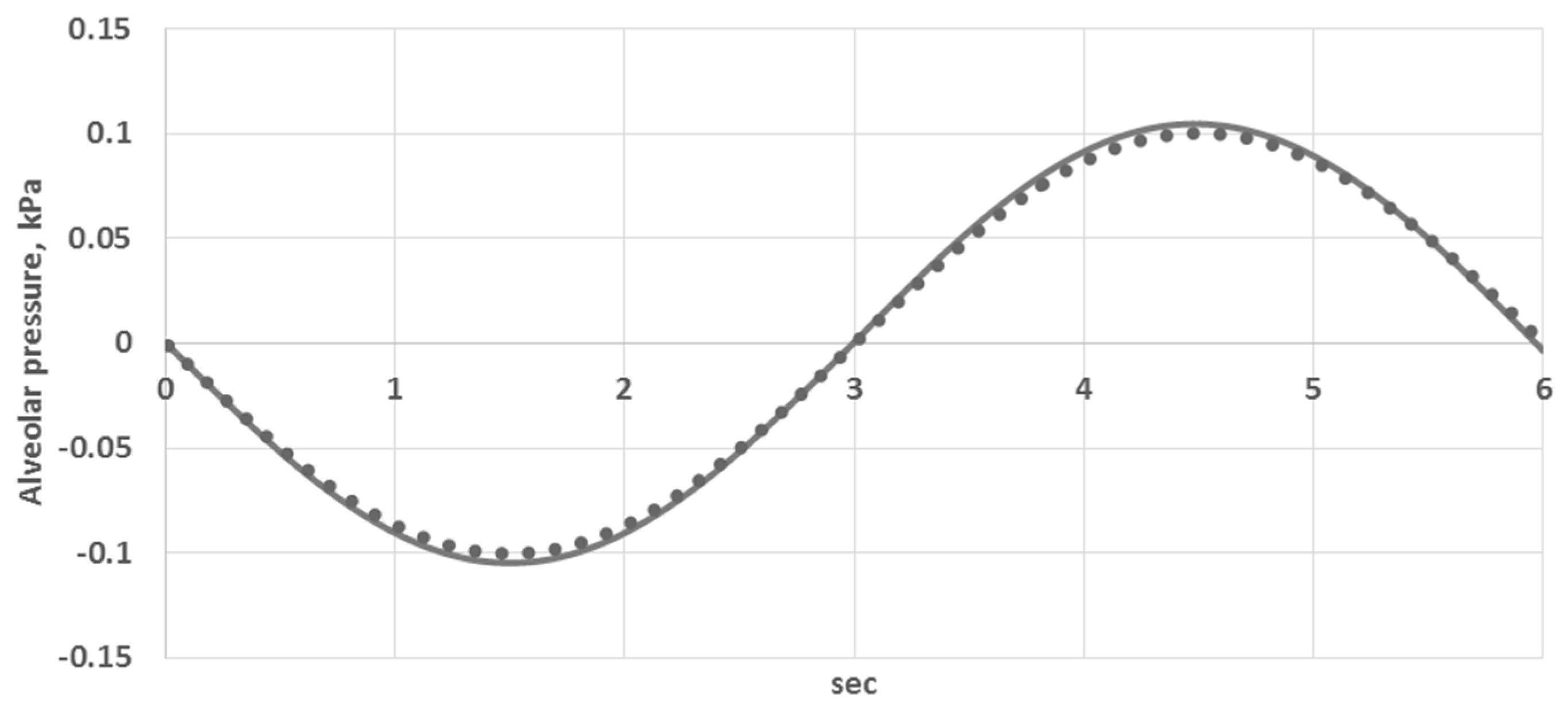
where V a k is the volume of the bronchoalveolar compartment, which is varied in time according to Equation (9). Equation (14) was substituted with Equation (9). This approach was validated by the comparison of the calculated and measured alveolar air flow and alveolar pressure (see Figure 2 and Figure 3 in Section 3.1.).
The boundary conditions at the bifurcations Equations (4) and (5), at the input to the nasopharyngeal region Equation (6) and at the junctions with bronchoalveolar compartments Equations (7)–(10) should be combined with compatibility conditions along the characteristics of a hyperbolic set Equations (1) and (2) leaving the integration domain. Here we outline the main aspects. More details can be found in [26,27]. Using the notation
V k = ( S k u k ) , F ( V k ) = ( S k u k u k 2 2 + p k ( S k ) ρ )
We can rewrite Equations (1) and (2) in a divergent form:
V k t + F ( V k ) x = 0
The eigenvalues λ k and left eigenvectors w k of the Jacobi matrix A k = F k V k = { F k i V k j } i , j = 1 2 are:
λ k i = u k + ( 1 ) i S k ρ p k S k = u k + ( 1 ) i c 0 k S k S 0 k , i = 1 , 2
w k i = ( 1 ρ p k S k ( 1 ) i S k ) = ( c 0 k S 0 k ( 1 ) i S k ) ,   i = 1 , 2 .
Compatibility conditions of Equations (1) and (2) along characteristics are:
w k i ( d V k d t ) i = w k i ( V k t + λ k i V k x ) = 0 ,   i = 1 , 2
In the case of respiratory mechanics both in normal and pathological conditions: | u k | < c 0 k S k S 0 k ; furthermore, there exists one positive and one negative eigenvalue and one incoming and one outgoing characteristic at the entrance and the output of every bronchial tube. Every set of boundary conditions, as described above, must be combined with Equation (19) for every incoming and outgoing tube. For the incoming tube, positive eigenvalue must be taken ( i = 2 , positive slope), for the outgoing tube, negative eigenvalue must be taken ( i = 1 , the negative slope).

2.3. Mathematical Model of the Oxygen and Carbon Dioxide Transport in the Lung

The transport of oxygen and carbon dioxide associated with the 1D flow is described by the convection equation:
C k , m t + u k C k , m x = 0
where m is the index of the substance; C k , m is the fraction (concentration) of the substance m in the k t h tube. The boundary conditions at the junctions of the bronchial tubes are set as a mass conservation condition:
C k 1 n , m ( t , L k 1 n ) S k 1 n ( t , L k 1 n ) u k 1 n ( t , L k 1 n ) = = C k 2 n , m ( t , 0 ) S k 2 n ( t , 0 ) u k 2 n ( t , 0 ) + C k 3 n , m ( t , 0 ) S k 3 n ( t , 0 ) u k 3 n ( t , 0 )
If u k j n ( t , x ˜ k j n ) > 0 , then C k j n , m is derived from Equation (20) along outgoing characteristic. If u k j n ( t , x ˜ k j n ) < 0 , then
C k j n , m ( t , x ˜ k j n ) = C n , m n o d e
where C n , m n o d e is concentrated at the junction, which is derived from Equation (21). The boundary conditions at the input to the nasopharynx during inspiration ( u 1 ( t , 0 ) > 0 ) are set as:
C 1 , O 2 ( t , 0 ) = C O 2 a t m ,   C 1 , C O 2 ( t , 0 ) = C C O 2 a t m ,
or derived from Equation (20) if u 1 ( t , 0 ) < 0 (expiration).
At the outputs of terminal bronchial tubes concentration, C k , m ( t , L k ) is derived from Equation (20), if u k ( t , L k ) > 0 , or is calculated together with the model of the gas exchange between the bronchoalveolar compartment and the blood:
C k , m ( t , L k ) = C a , m k ,  if  u k ( t , L k ) < 0
d ( C a , m k V a k ) d t = C k , m S k ( t , L k ) u k ( t , L k ) + D m S a k ( C m b C a , m k )
d C m b d t = Q m b V b + D m k S a k V b ( C a , m k C m b )
where k is in the range of the indices of bronchoalveolar compartments (in this work k = 8 , ... , 15 , see Figure 1b); C a , m k is the m t h substance fraction in k t h bronchoalveolar compartment; D m is the coefficient of the diffusion of m t h substance between bronchoalveolar compartment and the blood; C m b is the m t h substance fraction in the blood; Q m b is the source or sink of the m t h substance corresponding to the physiological conditions of the body; V b is the total volume of the blood in the body; S a k is the effective area of the surface of bronchoalveolar compartment, which is calculated as:
S a k = 36 π ( V a k ) 2 3

2.4. Numerical Implementation

From the mathematical standpoint, the 1D model of respiratory gas flow in the tracheobronchial tree is similarly to the 1D model of a blood flow in a network of vessels. This is a set composed of pairs Equations (1) and (2) of nonlinear hyperbolic equations for every bronchial tube. These pairs are joined together through non-linear algebraic equations which are derived from the boundary conditions at the inlet Equation (6) or finite difference discretization of the conditions at the outlets Equations (7)–(9) and at the junctions Equations (4) and (5). Every set is extended by the finite difference discretization of the appropriate compatibility condition Equation (19) in each of the above cases.
Fractional time steps, implicit−explicit algorithm allows splitting computations into several stages. The grid-characteristic finite difference method [32] was successfully applied to both respiratory gas flow and blood flow models [33,34,35,36]. At the first (explicit) stage, we use the first-order explicit monotonic implementation of this method for solving the set Equations (1) and (2) at every time step at the internal nodes of the numerical grid of every bronchial tube. At the second (implicit) stage, we solve the non-linear algebraic equation sets at the inlet, outlets and junctions by Newton’s method for the terminal nodes of the numerical grid of every bronchial tube. This set is constructed using finite difference discretization of Equation (19), which is based on the values of neighboring internal grid nodes calculated at the first stage. Null approximation for the iterations at the second stage is taken from the previous time step which is partly validated convergence of Newton’s method, since the time step is relatively small. Practically, no more than five iterations were required to achieve convergence up to 10 6 relative error for all simulations in this work. Several other possible approaches have been reviewed in [36]. The main difference of the numerical implementation in this work concerns discretization of the boundary condition sets: Equations (4)–(9); compatibility conditions Equation (19) and the model of the of respiratory gasses transport Equations (20)–(27).
Compatibility conditions Equation (19) are discretized by the first-order implicit approximation using forward difference for the entrance to the bronchial tube ( x k = 0 ) and backward difference for the output of the bronchial tube ( x k = L k ) along the x axis and first-order implicit approximation along the t axis:
( V x ) 0 n + 1 = V 1 n + 1 V 0 n + 1 h ,   ( V x ) J n + 1 = V J n + 1 V J 1 n + 1 h ,
( V t ) p n + 1 = V p n + 1 V p n τ n + 1 , p = 0 , J
where V p n is an element of discrete function which is defined on the mesh and represents mesh analog for the V from Equation (15). This mesh is uniform along the x axis:
( x j , t n ) : x j = h j ; j = 0 , ... , J ; h J = L ; t n = p = 0 n 1 τ p
Time step is selected on the basis of stability requirement imposed by the numerical method for Equations (1) and (2):
τ n + 1 = 0.9 max k = 1 , ... , K ; i = 1 , 2 | λ k i n | h k
where K is the total number of bronchial tubes. Finally, Equation (19) can be discretized as
( w i ) p n ( V p n + 1 V p n τ n + 1 + ( λ i ) p n V p n + 1 V q n + 1 h ) = 0 , ( i , p , q ) { ( 1 , 0 , 1 ) , ( 2 , J , J 1 ) }
There exists an obvious one-to-one mapping between the p and the triplet ( i , p , q ) . Thus, we use shorter notation p = 0 , J instead of the full notation ( i , p , q ) . Using the notations:
α p n = ( 1 ) i + 1 c 0 S p n S 0 ,   β p n = u p n + ( 1 ) i σ p n u q n α p n ( S p n + ( 1 ) i σ p n S q n ) 1 + ( 1 ) i σ p n , σ p n = τ n + 1 h ( λ i ) p n
Equation (32) can be rewritten as:
u p n + 1 = α p n + 1 S p n + 1 + β p n + 1 , p = 0 , J
Finally, the discretization of the boundary conditions at the bronchial tube junctions Equations (4), (5) and (19) can be reduced to the set of three quadratic equations in the form:
s I I = A s + b
where s = ( S k 1 ( t n + 1 , L k 1 ) , S k 2 ( t n + 1 , 0 ) , S k 3 ( t n + 1 , 0 ) ) T , s I I = ( S k 1 2 ( t n + 1 , L k 1 ) , S k 2 2 ( t n + 1 , 0 ) , S k 3 2 ( t n + 1 , 0 ) ) T , coefficients of A and b are derived from Equations (4), (5), (34) and depend on α p , β p and constants of the model (see Table A1).
Discretization of the cross-section area at the inlet to the tracheobronchial tree can be derived by substituting Equation (3) with Equation (6):
( S 1 ) 0 n + 1 = ( 1 + p a t m ρ w c 01 2 ) S 01
and using Equation (34) to compute ( u 1 ) 0 n + 1 .
Discretization of the boundary conditions at the outlets of the tracheobronchial tree (junctions of the bronchioles and bronchoalveolar compartment) can be derived as follows: (7) is integrated over a time step by the implicit Euler method as:
V a n + 1 = V a n + τ S J n + 1 u J n + 1
Equations (7), (8) and (37) are used to rewrite Equation (9) as:
128 η 9 π 2 ( V a n + τ S J n + 1 u J n + 1 ) S J n + 1 u J n + 1 + E a ( V a n + τ S J n + 1 u J n + 1 V 0 a ) = ρ c 0 2 ( S J n + 1 S 0 1 ) p p l n + 1
Substitution of Equation (32) with Equation (36) results in the fourth-order polynomial equation for the only unknown variable, S J n + 1 , which is solved by Newton’s method starting from the value S J n as null approximation. This is sufficient for the convergence as the time steps, which are limited by the stability condition Equation (31), are sufficiently small relative to the respiratory cycle ( τ 10 4 s ) .
The model of respiratory gas transport in Equations (20)–(27) is discretized by implicit methods after the values of the airflow were calculated by the above methods. Thus, the values of the area cross-section, linear velocity and alveolar volume at the upper time layer ( t = t n + 1 ) are known. The numerical algorithm is split for: processing the internal nodes of the bronchial tubes (Equation (20)); boundary conditions at the junctions of the bronchial tubes (Equations (21) and (22)); input to the nasopharynx (Equation (23)); junctions of the terminal bronchial tubes and bronchoalveolar compartments (Equations (24)–(27)) which are extended, if required, with the implicit discretization of Equation (20) derived at the appropriate terminal point (input or output of the bronchial tube) if the airflow velocity is directed outside the tube at this point.

2.5. Computed Tomography (CT) Data Processing

Initial 3D bronchial tube structure was segmented manually from an anonymous CT dataset. It was used as a source for automatic generation of 1D core network in 3D space and corresponding graph structure. Algorithm from [37] was applied. It was initially introduced and successfully applied for processing of patient-specific vascular networks. The algorithm consists of skeletonizing phase and graph structure generation phase. The first stage of the skeletonizing phase is a variant of the distance-ordered homotopic thinning (DOHT) algorithm [38], which produces as an output the initial skeleton of the input 3D image. Artificial structures in the form of short segments (twigs) may be also generated during this stage. The second stage was developed in order to remove such noise from the structure (see [37] for more details). In the second phase, the voxels of the skeletonized structure are divided into two groups: inner voxels (i.e., voxels adjacent to exactly two other skeletal voxels) and nodal voxels (other voxels). In this work, it was assumed that each voxel had 26 adjacent voxels. Finally, the groups of inner voxels were converted to the edges of the graph and nodal voxels were converted to the graph vertices. The average diameter and the actual length were computed following the above workflow and saved as attributes of the graph edges. Manual 3D segmentation and automatic 1D core network construction results are shown in Figure 1a,b. Network parameters are presented in Table A2.

3. Results

3.1. The Model Validation

The constants and parameters of the model are presented in Table A1 and Table A2. They were identified according to the processing of the anatomical CT data (see Section 2.5), literature data [18,26,29,30,31] and model validation with the data from [29]. The previous work on validation is presented in [26,32,33,34]. The major parameters of the lung ventilation affecting the alveolar gas exchange are the alveolar air flow and alveolar pressure. Thus, in this work, we additionally performed simulations of the dynamical change of the total air flow at the trachea (flux at the terminal point of tube No. 1 in Figure 1) and alveolar pressure (pressure at the bronchoalveolar compartments averaged over the compartments). The results are shown in Figure 2 and Figure 3. The calculated data (designated by dots) are compared to the data from [29] (designated by curve). It is obvious from Figure 2 and Figure 3 that a reliable quantitative agreement is achieved.

3.2. Carbon Dioxide Elimination Efficiency during Artificial Ventilation

Artificial ventilation is widely used in surgery for maintaining vital conditions during anesthesia. Generally, artificial ventilation parameters (tidal volume and respiratory rate) are manually controlled by the anesthesiologist based on a patient’s vitals. The main task of the anesthesiologist is to maintain vital functions of the organism providing sufficient O 2 supply and CO 2 elimination through the lung. Certain parameters are not directly assayed and monitored during a surgical procedure with general anesthesia, such as arterial blood CO 2 concentration. Understanding of the relationship between parameters of the artificial ventilation and alveolar concentration of O 2 and CO 2 is very important in order to predict CO 2 elimination capacity of ventilation. In this section, we perform in silico study of the alveolar CO 2 concentration dependence on the respiratory rate changes. The following assumptions are made. The minute volume ( V minute ) was fixed and tidal volume ( V t d ) was derived from:
60 V t d ν A R R = V m i n u t e = c o n s t
The pleural pressure in Equation (10) was “switched off” ( p g = 0 ) and the nasopharyngeal pressure in Equation (6) was varied as:
S 1 ( t , 0 ) u 1 ( t , 0 ) = Q t d sin ( 2 π ν A R R t ) , Q t d = V t d / 0 T / 2 sin ( 2 π ν A R R t ) d t = V t d π ν A R R
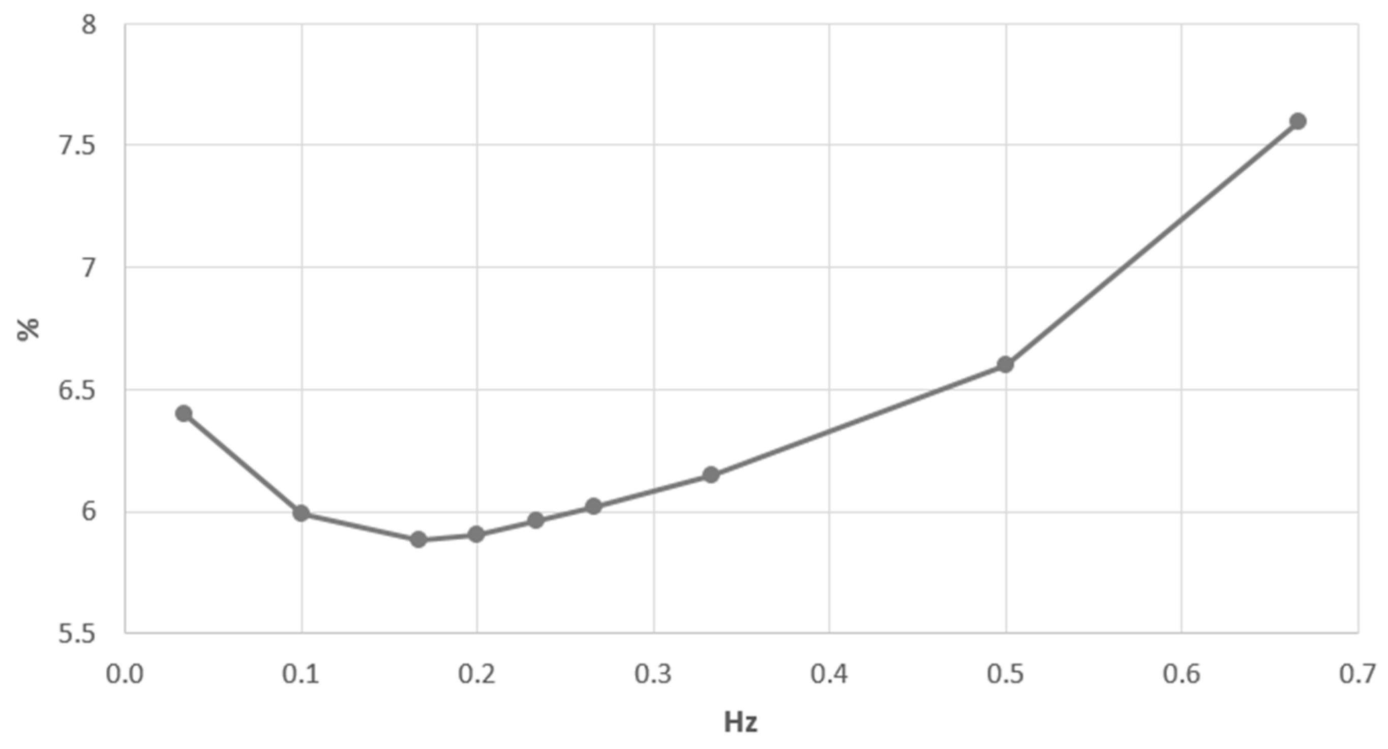
where ν A R R is the frequency of the artificial respiratory rate (ARR), and Q t d is the amplitude of the inhaled airflow. The ARR was varied in the acceptable physiological range ( 0 < ν A R R < 0.7 H z ) . The CO 2 concentration in alveolar volume was simulated by the integrated model presented in Section 2 and averaged over several cycles of ARR. The results are shown in Figure 4.
The minimum value of CO 2 concentration is considered as a criterion of the effective lung functioning during artificial ventilation. The initial increase of the ARR from zero is associated with the increase of CO 2 elimination and with the decrease of CO 2 concentration (Figure 4). The minimum is achieved at the ARR frequency of 0.17 Hz, which is very close to the measured frequency of the quiet breathing of the patient (0.23 Hz). The further increase of ARR results in the increase of the CO 2 concentration. It can be explained by the tidal volume decrease Equation (39) and decreased alveolar pressure. Finally, the partial pressure gradient of CO 2 between the alveolar volume and the blood and the period of the gas exchange per cycle is decreased. It results in the decreased lung efficiency. The increase of ARR above optimal value is also associated with the earlier onset of the expiratory phase. Thus, the inspired gas with minimal CO 2 concentration could not fully achieve bronchoalveolar compartments. It also contributes to the increase of CO 2 concentration in the alveolar volume.

3.3. The Study of Pathological Breathing Patterns

In this work, we define breathing pattern as a time profile of pleural pressure (the function p p l ( t ) in Equation (10). The breathing pattern is an important characteristic of the respiratory system. It strongly affects the alveolar gas exchange effectiveness. In this section, we perform in silico study of the dependence of CO 2 concentration in the alveolar volume on the breathing pattern. We consider two types of pathological breathing patterns: cluster (Biot) and periodic (Cheyne-Stokes) breathings [39,40] and comparing them to the normal (sinusoidal) respiration [30]. Normal breathing was simulated as:
p p l ( t ) = p g sin ( v t )
Cluster breathing is a type of abnormal breathing pattern. We consider it as a group of sinusoidal inspirations followed by the period of apnea. It was simulated as:
p p l ( t ) = { 2 p g sin ( v t ) , 0 t < 0.5 T p t 0 , 0.5 T p t t < T p t
where T p t is the period of pattern and t is the time counted from the beginning of the period. Periodic breathing is a type of abnormal breathing pattern which is characterized by the non-synchronous contraction of the respiratory muscles. It was simulated as:
p p l ( t ) = { 2 p g sin ( v t ) sin ( 5 v t ) , 0 t < 0.75 T p t 0.1 p g sin ( v t ) , 0.75 T p t t < T p t
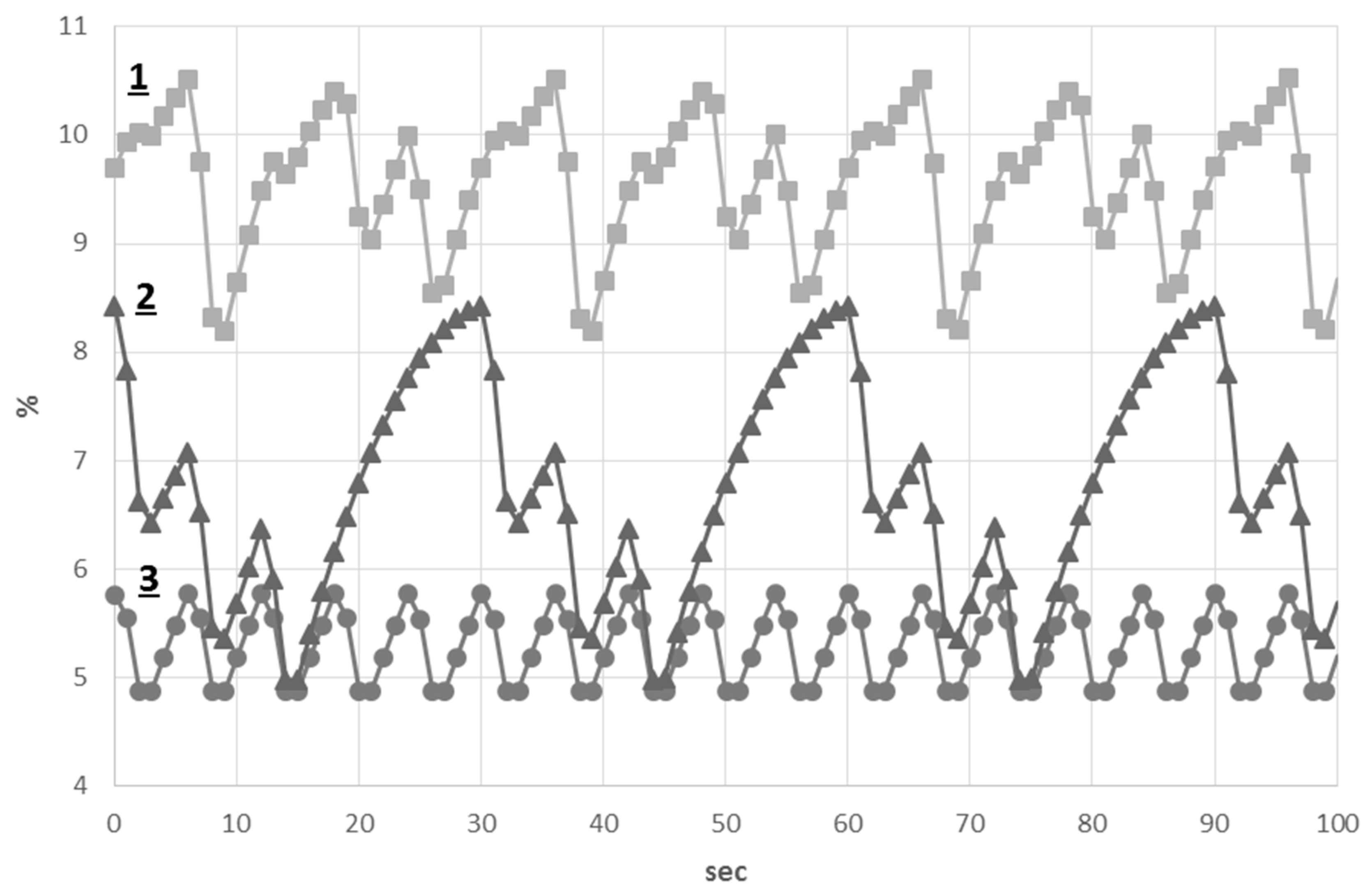
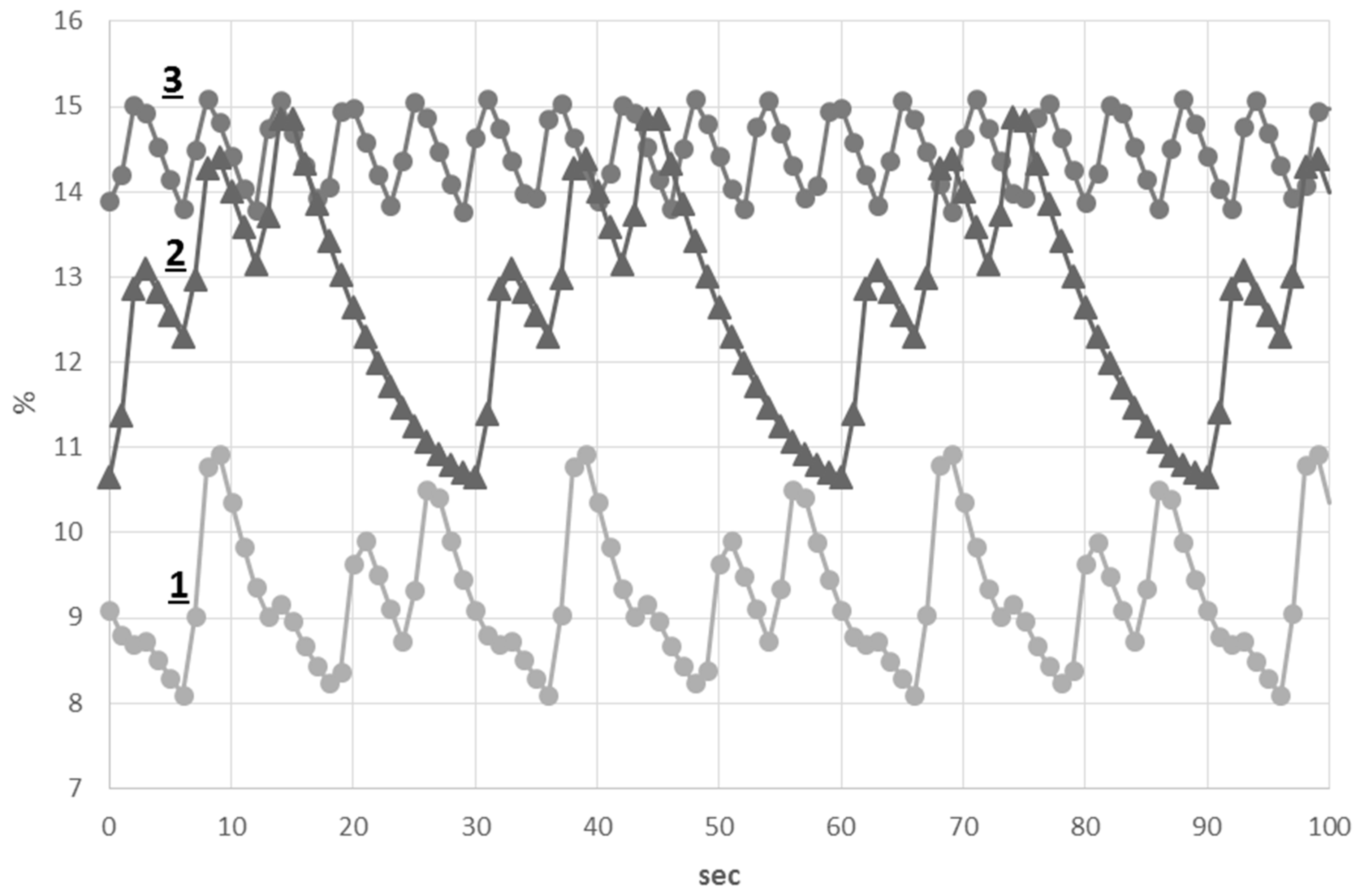
The results of the alveolar concentration of CO 2 and O 2 simulations are shown in Figure 5 and Figure 6. The alveolar CO 2 concentration remained within 4.8%–5.9% during normal breathing. Both cluster and periodic breathings significantly affect this value. The alveolar CO 2 concentration was increased up to 8.4% during cluster breathing, whereas a highly increased value of this parameter was found during periodic breathing (8%–10.4%). The alveolar O 2 concentration remained within 13.9%–15.1% during normal breathing. This value had a wider range during cluster breathing with its lowest value at 10.7%. A highly decreased value of the alveolar O 2 concentration was found during periodic breathing (8%–11%).
Thus, during periodic breathing, both alveolar CO 2 and O 2 values were substantially changed in comparison to those of normal and cluster breathings.

3.4. Asthma Model

Asthma is a chronic inflammatory disease of the respiratory system. Chronic inflammation leads to the progressing of bronchial hyperactivity, which is caused by a violation of the autonomic regulation of smooth muscle tone and the action of inflammatory mediators and leads to periodic reversible bronchial obstruction, which is caused by increased lung airway resistance. Due to the lung obstruction, some of the air is delayed in the alveoli, lungs are restretched, the residual volume is increased and the vital capacity is reduced. A mismatch between ventilation and perfusion leads to the increase of partial pressure of CO 2 and the decrease of O 2 in the blood.
Clinically, asthma attacks are classified as mild, moderate and severe [41]. In this work, asthma attack was simulated by reducing the reference cross-section area S 0 in Equation (3) for all terminal tubes and by reducing the effective radius of the alveolar volume r e f in Equation (12) as:
S 0 γ = π ( r e f γ ) 2 = S 0 n o r m ( 100 γ ) / 100
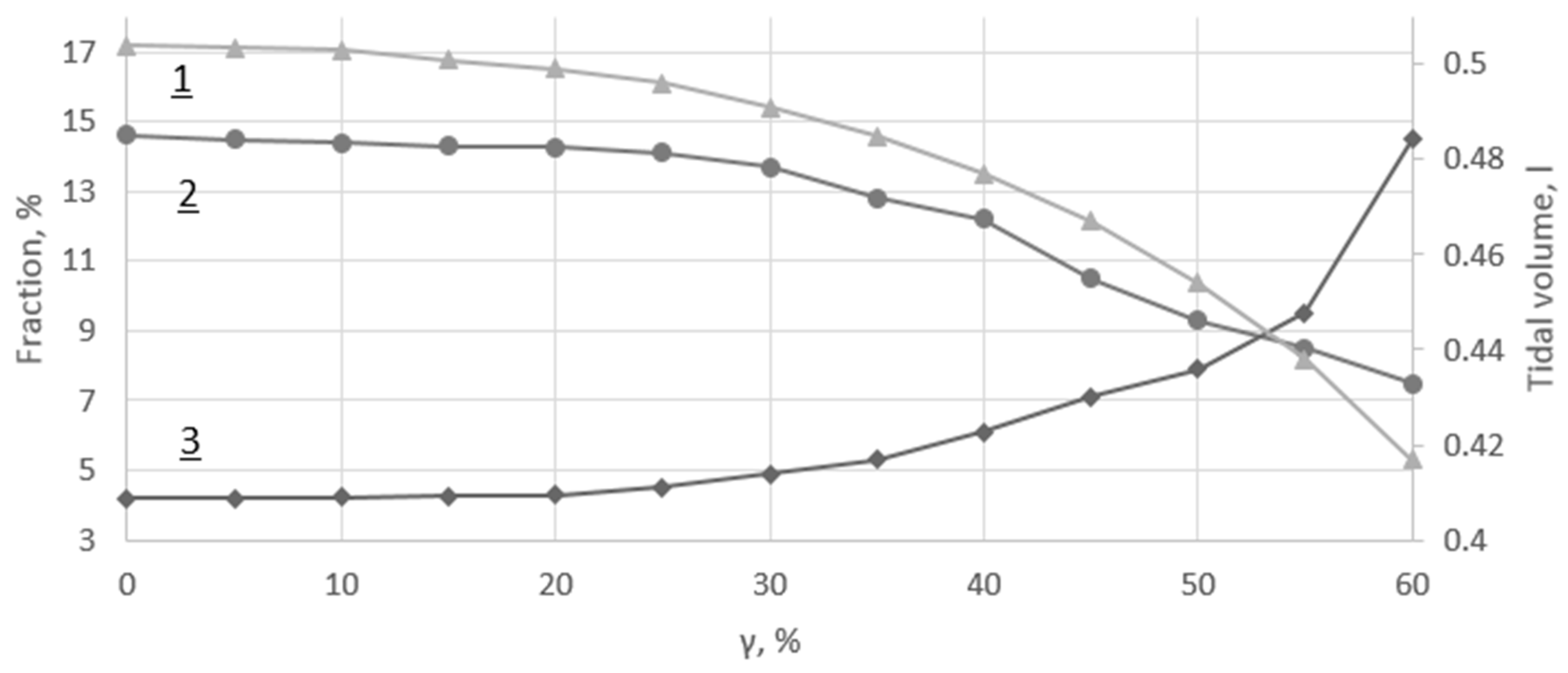
where S 0 γ , r e f f γ are modified reference cross-section and effective radius during the asthma attack; 0 % γ 100 % is a coefficient of asthma severity; γ = 0 % corresponds to the normal conditions; γ = 100 % corresponds to the full collapse of the terminal airways. The results of the simulations are shown in Figure 7.
Changes in parameters of tidal volume and alveolar O 2 concentration are slightly decreased over the mild attack range ( 0 % γ 20 % ), whereas alveolar CO 2 concentration remains stable (see Figure 7). The moderate attack range ( 20 % γ 40 % ) is characterized by noticeably decreased parameters of tidal volume and alveolar O 2 concentration, accompanied by a negatively correlated increase of alveolar CO 2 concentration. The severe attack range ( γ > 40 % ) is characterized by further dramatic changes in all of these parameters, which exceeds the physiological range in γ > 50 % . Thus, the upper limit of the severe asthma attack simulation range was γ = 50 % .
Thus, based on a computational model of the airflow and matter transfer in the lung with individual CT data analysis, the following simulating models were developed: (1) Model of CO 2 elimination efficiency during artificial ventilation; (2) Model of pathological breathing patterns (cluster (Biot) and periodic (Cheyne-Stokes) breathings) compared to the normal (sinusoidal) breathing pattern; (3) Asthma breathing model in cases of mild, moderate and severe attacks.

4. Discussion

Currently, in silico studies addressed to respiratory lung modeling have been covering detailed patient-specific 3D lung reconstruction [13,14], nasopharynx-trachea ventilation features [6,7,15], 3D-1D coupling of upper and middle airway segments, and FSI simulations [16]. The lumped models operate with lung mechanics in terms of tidal volume and pressure with lower details [17,18]. These models are used as boundary conditions for multiscale 3D−0D, 3D−1D−0D or 1D−0D simulations [9,19,20,21,22]. Some studies are devoted to simulations of blood biochemistry, including alveolar gas ( O 2 / CO 2 ) exchange [23,24,25].
To the best of our knowledge, the problem of individualized computational analysis of respiratory mechanics and alveolar gas balance during pathological conditions has been rarely addressed in the literature. Therefore, in this work, the 1D model of incompressible fluid flow through the network of the elastic tubes was used to simulate airflow in the first four generations of the tracheobronchial tree. It was coupled with 0D nonlinear models of lumped alveolar components, which aggregates parts of alveolar volume and smaller airways. The model also included a convective transport model throughout the lung and alveolar components. The main novel features of our work are: the use of automatic 1D reconstruction of the tracheobronchial tree structure on the basis of 3D segmentation of individual CT data; a new method of 1D−0D coupling of a 1D bronchial tube and 0D alveolar component; as well as an in silico study of the respiratory gas transport and balance during pathological conditions. Using the developed integrated multiscale model, we analyzed CO 2 elimination efficiency during artificial ventilation due to the pathological breathing patterns of both cluster and periodic breathings as well as the asthma attack.
Simulation of artificial ventilation was based on constant minute volume, variable breathing frequency and calculated tidal volume with the alveolar CO 2 concentration as an output value. According to the results of our simulations we suggest that the optimal value of the ventilation frequency is about 0 . 2   ±   0 . 05 Hz , which corresponds to the clinically measured value of normal breathing ( 0 . 23 Hz ). This value is also in agreement with the optimal ventilation frequency ( 0 . 23 Hz ) corresponding to the minimum work of breathing, which was presented in the work of breathing model based on the Otis equation [42].
The impact of pathological breathing patterns such as a cluster (Biot) and periodic (Cheyne-Stokes) respirations on alveolar CO 2 and O 2 concentrations was demonstrated by simulation setting of specific time profile to the pleural pressure function. The alveolar CO 2 concentration was increased up to 8.4% during cluster breathing, and with highly increased values during periodic breathing (8%–10.4%) in comparison with that of normal breathing. During periodic breathing, both alveolar CO 2 and O 2 values were substantially changed in comparison to those of normal and cluster breathings.
Asthma attack was simulated by reducing the reference cross-section area of the terminal bronchioles and the effective radius of the bronchoalveolar compartments. Changes in parameters of tidal volume and alveolar O 2 concentration are slightly decreased over the mild attack range, whereas alveolar CO 2 concentration remains stable. The moderate attack range is characterized by noticeably decreased parameters of tidal volume and alveolar O 2 concentration, which was accompanied by negatively correlated increase of alveolar CO 2 concentration. The severe attack range is characterized by further dramatic changes in all of these parameters.
Approximation of the hydraulic resistance given by Equation (14) is not precise. Nevertheless, this formulation allows consideration of each bronchoalveolar compartment independently. It provides a potential possibility for a correct simulation of the heterogeneous lung structure beyond the CT segmented region, which has not been implemented in this work. Equation (14) does not account for the smaller bronchial tubes’ properties in detail. The accuracy of this method would have been increased had better CT data quality been available, along with the increase of the CT segmented region covered by the 1D model.
The use of the first-order explicit numerical method for the 1D part of the model (see Section 2.4) resulted in the strict limitation on the time step due to stability conditions. The higher-order methods may be applied to the numerical discretization of this part of the model for the increase of the numerical efficiency. It would require the higher-order approximation of the compatibility conditions (see Equation (19)) and should be analyzed in the future. Current numerical implementation is still effective for clinical practice. The typical time of the simulations was not more than half an hour per case.
Our aim in the future is patient-specific analysis. We werelimited in this work by the data quality available from typical hospital CT scans that we extended with 0D compartments. The parameters of the reconstructed trachea-bronchial tree and 0D compartments should thus be validated by additional patient-specific data which were not available at the time of investigation. Identification of the parameters and model validation were performed on the basis of well-known literature on the physiology [18,29,30,31]. The results of the simulations demonstrated good quantitative agreement. It is clear that more patient-specific cases and validations are needed to be able to include this approach in clinical practice.

5. Conclusions

The results of our mathematical modeling of breathing patterns of severely ill patients with cluster and periodic respirations, as well as breathing patterns of patients with an asthma attack, demonstrated the suitability of our mathematical simulations by differentiating the individual properties of patients in each case. Further improvements of the model, however, are required, and should include: heterogeneous anatomy of the left and right lobes; non-linear elasticity of parenchymal tissue; higher-order numerical discretization of 1D; automatic patient-specific parameter identification and validation; and sufficient patient-specific simulations.
In the future, the results of our study could be integrated into research and practical studies aimed to design cyberbiological systems for offline analysis and real-time monitoring of respiration parameters including their monitoring, individualized classification and prediction of breathing patterns, in addition to analysis of alveolar gas exchange for patients with breathing problems (e.g., patients after surgical interventions and other high-risk patients).

Acknowledgments

The work was supported by the Russian Science Foundation, grant No. 14-11-00877. The method of CT data processing (Section 2.5) and the results shown in Figure 1 and Table A2, were obtained under the support of the Russian Science Foundation, grant No. 14-31-00024. The authors acknowledge Dmitry V. Burenchev for the patient-specific data of the tracheobronchial tree.

Author Contributions

S.S., A.K., O.A. designed the study concept; S.S. and A.K. developed the model of respiratory gas flow in the tracheobronchial tree, S.S., A.G. and Y.N.S. developed the model of alveolar dynamics and gas exchange with the arterial blood; A.G. and Y.N.S. performed simulations; S.S., O.A. and A.K. analyzed the results; R.P. processed patient-specific data and prepared 1D network structure for simulations; S.S., A.K. and O.A. interpreted clinical applications of simulations; S.S., A.G., R.P., Y.N.S., O.A., A.K. drafted the manuscript and all authors equally participated in revising and approving the final manuscript for publication.

Conflicts of Interest

The authors declare no conflict of interest.

Abbreviations

The following abbreviations are used in this manuscript:
CTComputed tomography
FSIFluid-structure interaction
ARRArtificial respiratory rate

Appendix A

Table A1. Constants of the model.
SymbolValueUnit
ρ 1.23 × 10⁻⁶ kg / cm 3
η 1.8 × 10⁻³ kg / ( cm s )
θ O 2 0.17 cm 2 / s
θ CO 2 0.16 cm 2 / s
D O 2 1.2 × 10⁻³ l / s
D CO 2 6.7 × 10⁻² l / s
E a 0.5 kPa / l
ν 0.16 Hz
V 0 t o t 5 l
p g 1.3 kPa
p a t m 101.3 kPa
V b l o o d 4 l
V m i n u t e 5 l
Q O 2 b 0.25 l / min
Q CO 2 b 0.2 l / min
C O 2 a t m 0.209
C CO 2 a t m 2.8 × 10⁻⁴
T p t 1 min
Table A2. Parameters of the 1D structure of the tracheobronchial tree (Figure 1b).
IndexLength, cm Diameter, cm c 0 , cm / s
112.491.387700
25.410.877382
32.861.117382
41.250.687064
51.630.667064
62.450.847064
71.820.537064
82.320.256747
91.50.476747
103.860.266747
111.020.436747
122.10.446747
130.60.646747
140.540.46747
151,290.276747

References

  1. Agache, I.; Ciobanu, C.; Paul, G.; Rogozea, L. Dysfunctional breathing phenotype in adults with asthma—Incidence and risk factors. Clin. Transl. Allergy 2012, 2, 18. [Google Scholar] [CrossRef] [PubMed]
  2. Folgering, H. The pathophysiology of hyperventilation disorder. Monalsi. Arch. Chest. Dis. 1999, 54, 365–371. [Google Scholar]
  3. Howell, J.B. Behavioural breathlessness. Thorax 1990, 45, 287–292. [Google Scholar] [CrossRef] [PubMed]
  4. Han, J.N.; Stegen, K.; Schepers, R.; Van den Bergh, O.; Woestinjne, K.P. Subjective symptoms and breathing pattern at rest and following hyperventilation in anxiety and somatiform disorders. J. Psychosom. Res. 1998, 45, 519–532. [Google Scholar] [CrossRef]
  5. Fekr, A.R.; Janidarmian, M.; Radecka, K.; Zilic, Z. A medical cloud-based platform for respiration rate measurement and hierarchical classification of breath disorders. Sensors 2014, 14, 11204–11224. [Google Scholar] [CrossRef] [PubMed]
  6. Longest, P.W.; Tian, G.; Delvadia, R.; Hindle, M. Development of a stochastic individual path (SIP) model for predicting the deposition of pharmaceutical aerosols: Effects of turbulence, polydisperse aerosol size, and evaluation of multiple lung lobes. Aerosol Sci. Technol. 2012, 46, 1271–1285. [Google Scholar] [CrossRef]
  7. Comerford, A.; Gravemeier, V.; Wall, W.A. An algebraic variational multiscale-multigrid method for large-eddy simulation of turbulent pulsatile flows in complex geometries with detailed insight into pulmonary airway flow. Int. J. Numer. Meth. Fluids 2013, 71, 1207–1225. [Google Scholar] [CrossRef]
  8. Tian, G.; Longest, P.W.; Su, G.; Walenga, R.L.; Hindle, M. Development of a Stochastic Individual Path (SIP) Model for Predicting the Tracheobronchial Deposition of Pharmaceutical Aerosols: Effects of Transient Inhalation and Sampling the Airways. J. Aerosol Sci. 2011, 42, 781–799. [Google Scholar] [CrossRef]
  9. Ismail, M.; Comerford, A.; Wall, W.A. Coupled and reduced dimensional modelling of respiratory mechanics during spontaneous breathing. Int. J. Numer. Meth. Biomed. Eng. 2013, 29, 1285–1305. [Google Scholar] [CrossRef] [PubMed]
  10. Roth, C.J.; Ismail, M.; Yoshihara, L.; Wall, W.A. A comprehensive computational human lung model incorporating inter-acinar dependencies: Application to spontaneous breathing and mechanical ventilation. Int. J. Numer. Meth. Biomed. Eng. 2017, 33, e02787. [Google Scholar] [CrossRef] [PubMed]
  11. Tian, G.; Longest, P.W.; Su, G.; Hindle, M. Characterization of Respiratory Drug Delivery with Enhanced Condensational Growth Using an Individual Path Model of the Entire Tracheobronchial Airways. Ann. Biomed. Eng. 2011, 39, 1136–1153. [Google Scholar] [CrossRef] [PubMed]
  12. Longest, P.W.; Holbrook, L.T. In Silico Models of Aerosol Delivery to the Respiratory tract—Development and Applications. Adv. Drug Deliv. Rev. 2012, 64, 296–311. [Google Scholar] [CrossRef] [PubMed]
  13. Kleinstreuer, C.; Feng, Y. Lung Deposition Analyses of Inhaled Toxic Aerosols in Conventional and Less Harmful Cigarette Smoke: A Review. Int. J. Environ. Res. Public Health 2013, 10, 4455–4458. [Google Scholar] [CrossRef] [PubMed]
  14. Lin, J.; Hu, G.L.; Fan, J.R.; Pan, D. Study on Airflow and Inhaled Particle Deposition within Realistic Human Upper Respiratory Tract. J. Phys. Conf. Ser. 2009, 147, 1–10. [Google Scholar] [CrossRef]
  15. Tena, A.F.; Casan, P.; Fernandez, J.; Ferrera, C.; Marcos, A. Characterization of particle deposition in a lung model using an individual path. EPJ Web Conf. 2013, 45, 1–5. [Google Scholar] [CrossRef]
  16. Ilegbusi, O.J.; Li, Z.; Seyfi, B.; Min, Y.; Meeks, S.; Kupelian, P.; Santhanam, A.P. Modeling Airflow Using Subject-Specific 4DCT-Based Deformable Volumetric Lung Models. Int. J. Biomed. Imag. 2012, 2012, 1–10. [Google Scholar] [CrossRef] [PubMed]
  17. Crooke, P.S.; Hotchkiss, J.R.; Marint, J.J. Linear and Nonlinear Mathematical Models for Noninvasive Ventilation. Math. Comput. Mod. 2002, 35, 1297–1313. [Google Scholar] [CrossRef]
  18. Ben-Tal, A. Simplified Models for Gas Exchange in the Human Lungs. J. Theor. Biol. 2006, 238, 474–495. [Google Scholar] [CrossRef] [PubMed]
  19. Comerford, A.; Förster, C.; Wall, W.A. Structured tree impedance outflow boundary conditions for 3D lung simulations. ASME J. Biomech. Eng. 2010, 132. [Google Scholar] [CrossRef] [PubMed]
  20. Lin, C.-L.; Tawhai, M.H.; McLennan, G.; Hoffman, E.A. Multiscale simulation of gas flow in subjectspecific models of the human lung. IEEE Eng. Med. Biol. 2009, 28, 25–33. [Google Scholar]
  21. Polak, A.G.; Lutchen, K.R. Computational Model for Forced Expiration from Asymmetric Normal Lungs. Ann. Biomed. Eng. 2003, 31, 891–907. [Google Scholar] [CrossRef] [PubMed]
  22. Malve, M.; del Palomar, A.P.; Chandra, S.; López-Villalobos, J.L.; Mena, A.; Finol, E.A.; Ginel, A.; Doblaré, M. FSI Analysis of a Healthy and a Stenotic Human Trachea Under Impedance-Based Boundary Conditions. J. Biomech. Eng. 2011, 133, 1–12. [Google Scholar] [CrossRef] [PubMed]
  23. Brighenti, C.; Gnudi, G.; Avanzolini, G. A simulation model of the oxygen alveolo-capillary exchange in normal and pathological conditions. Physiol. Meas. 2003, 24, 261–275. [Google Scholar] [CrossRef] [PubMed]
  24. Reynolds, A.; Ermentrout, G.B.; Clermont, G. A mathematical model of pulmonary gas exchange under inflammatory stress. J. Theor. Biol. 2010, 264, 161–173. [Google Scholar] [CrossRef] [PubMed]
  25. Schulz, K.G.; Riebesell, U.; Rost, B.; Thoms, S.; Zeebe, R.E. Determination of the rate constants for the carbon dioxide to bicarbonate inter-conversion in pH-buffered seawater systems. Mar. Chem. 2006, 100, 53–65. [Google Scholar] [CrossRef] [Green Version]
  26. Simakov, S.S.; Kholodov, A.S. Computational study of oxygen concentration in human blood under low frequency disturbances. Math. Models Comput. Simul. 2009, 1, 283–295. [Google Scholar] [CrossRef]
  27. Kholodov, Y.A.; Kholodov, A.S.; Kovshov, N.V.; Simakov, S.S.; Severov, D.S.; Bordonos, A.K.; Bapayev, A. Computational models on graphs for nonlinear hyperbolic and parabolic system of equations. In III European Conference on Computational Mechanics; MotaSoares, C.A., Martins, J.A.C., Rodrigues, H.C., Ambrósio, J.A.C., Pina, C.A.B., Motasoares, C.M., Pereira, E.B.R., Folgado, J., Eds.; Springer: Dordrecht, The Netherlands, 2006; p. 43, CD-ROM ID 2279. [Google Scholar]
  28. Pedley, T.J.; Luo, X.Y. Modelling Flow and Oscillations in Collapsible Tubes. Theor. Comput. Fluid Dyn. 1998, 10, 277–294. [Google Scholar] [CrossRef]
  29. Schmidt, R.F.; Thews, G. Human Physiology, 2nd ed.; Springer: Berlin, Germany, 1989; pp. 600–605. [Google Scholar]
  30. Mead, J. Mechanical properties of lungs. Physiol. Rev. 1961, 41, 281–330. [Google Scholar] [PubMed]
  31. Hamid, Q.; Shannon, J.; Martin, J. Physiologic Basis of Respiratory Disease; BC Decker Inc.: Hamilton, ON, Canada, 2005. [Google Scholar]
  32. Magomedov, K.M.; Kholodov, A.S. Grid-Characteristic Numerical Methods; Nauka: Moscow, Russia, 1988. (In Russian) [Google Scholar]
  33. Kholodov, A.S. Some dynamic models of external breathing and blood circulation with consideration for their coherence and mass transfer. In Computer Models and Medicine Progress; Belotserkovskii, O.M., Kholodov, A.S., Eds.; Nauka: Moscow, Russia, 2001; pp. 127–163. (In Russian) [Google Scholar]
  34. Simakov, S.S.; Kholodov, A.S.; Kholodov, Y.A.; Nadolskiy, A.A. Computational study of the vibrating disturbances to the lung function. In III European Conference on Computational Mechanics; MotaSoares, C.A., Martins, J.A.C., Rodrigues, H.C., Ambrósio, J.A.C., Pina, C.A.B., Motasoares, C.M., Pereira, E.B.R., Folgado, J., Eds.; Springer: Dordrecht, The Netherlands, 2006; p. 205, CD-ROM, ID 1467. [Google Scholar]
  35. Vassilevski, Y.; Simakov, S.; Dobroserdova, T.; Salamatova, V. Numerical issues of modelling blood flow in networks of vessels with pathologies. Russ. J. Numer. Anal. Math. Mod. 2011, 26, 605–622. [Google Scholar] [CrossRef]
  36. Bessonov, N.; Sequeira, A.; Simakov, S.; Vassilevski, Y.; Volpert, V. Methods of Blood Flow Modelling. Math. Mod. Nat. Phenom. 2016, 11, 1–25. [Google Scholar] [CrossRef]
  37. Danilov, A.; Ivanov, Y.; Pryamonosov, R.; Vassilevski, Y. Methods of graph network reconstruction in personalized medicine. Int. J. Numer. Meth. Biomed. Eng. 2016, 32. [Google Scholar] [CrossRef] [PubMed]
  38. Pudney, C. Distance-ordered homotopic thinning: A skeletonization algorithm for 3D digital images. Comput. Vis. Image Underst. 1998, 72, 404–413. [Google Scholar] [CrossRef]
  39. Wijdicks, E.F. Biot’s breathing. J. Neurol. Neurosurg. Psychiatry 2007, 78, 512–513. [Google Scholar] [CrossRef] [PubMed]
  40. Pearce, J.M.S. Cheyne-Stokes respiration. J. Neurol. Neurosurg. Psychiatry 2002, 72, 595. [Google Scholar] [CrossRef]
  41. Colice, G.L. Categorizing Asthma Severity: An Overview of National Guidelines. Clin. Med. Res. 2004, 2, 155–164. [Google Scholar] [CrossRef] [PubMed]
  42. Chang, D.W. Clinical Application of Mechanical Ventilation, 4th ed.; CENGAGE Learning: Boston, MA, USA, 2014; p. 105. [Google Scholar]
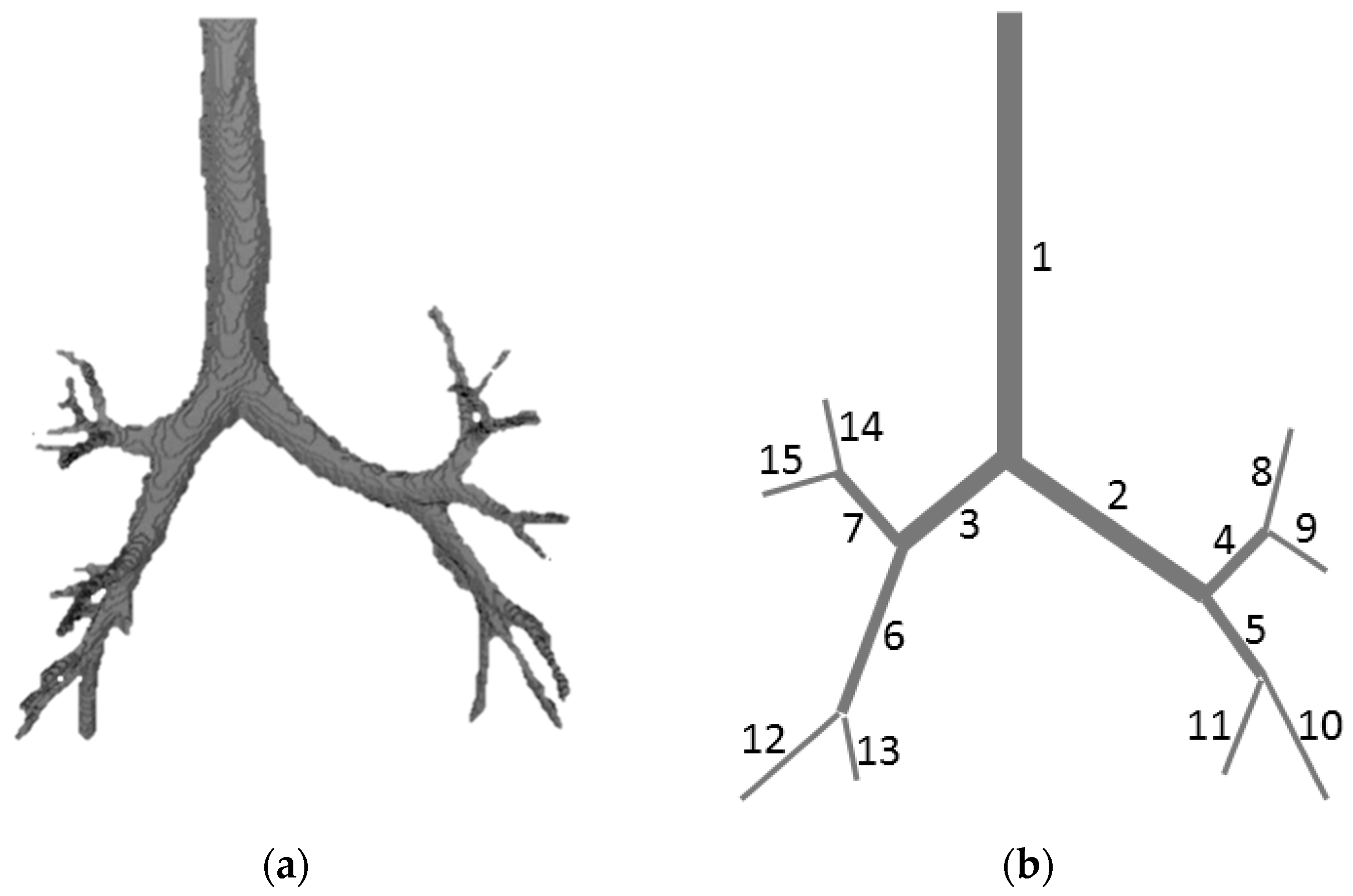
Figure 1. (a) 3D segmentation of the individual computed tomography (CT) data of the tracheobronchial tree; (b) 1D structure based on the 3D segmentation.
Computation 05 00011 g001
Figure 2. Comparison of the calculated and measured alveolar air flow (L/sec): curve—the data from [29], dots—simulations.
Computation 05 00011 g002
Figure 3. Comparison of the calculated and measured alveolar pressure (kPa): curve—the data from [29], dots—simulations.
Computation 05 00011 g003
Figure 4. Alveolar concentration of CO 2 from the artificial respiratory rate (ARR).
Computation 05 00011 g004
Figure 5. Alveolar concentration of CO 2 : (1) Periodic breathing; (2) Cluster breathing; (3) normal breathing.
Computation 05 00011 g005
Figure 6. Alveolar concentration of O 2 : (1) Periodic breathing; (2) Cluster breathing; (3) normal breathing.
Computation 05 00011 g006
Figure 7. (1) Tidal volume; (2) Alveolar O 2 concentration; (3) Alveolar CO 2 concentration.
Computation 05 00011 g007