Generalization of Defense Effects Learned from a Single Adversarial Attack

Abstract

Adversarial attacks misled deep neural networks by injecting perturbations into input images. Training networks with adversarial examples defended against adversarial attacks. However, training with specific adversarial examples only defended against the corresponding attacks. To generalize the defense effect from one specific attack to other attacks, we proposed a method called Gradient Vicinity Adversarial Training (GVAT), which generated adversarial examples along directions sampled in the vicinity of the gradient. The defense effects of GVAT were evaluated using three attack methods: fast gradient sign method (FGSM), projected gradient descent (PGD), and Carlini–Wagner (CW) under the $L_2$-norm constraint. A three-layer convolutional network was trained on the MNIST dataset, and two WideResNet-28-10 networks were trained on the CIFAR-10 and CIFAR-100 datasets respectively. Under the transfer-based black-box setting, the results showed that GVAT not only defended against the corresponding attacks that generated adversarial examples but also defended against other attacks. In other words, the defense effect of GVAT was generalized to other attacks under the transfer-based black-box setting.

1. Introduction

Deep neural networks achieved remarkable progress in a wide range of tasks and were widely applied to tasks such as image classification [1,2], autonomous driving [3,4], and speech recognition [5,6].

However, previous studies had shown that deep neural networks were vulnerable to adversarial examples. Szegedy et al. [7] first noticed that carefully crafted imperceptible perturbations added to input images could mislead models into making incorrect predictions. The perturbations referred to the input modifications added to the original example. Such perturbations were typically generated along the gradient direction that maximized the attack’s effectiveness. The direction of the gradient was given by the gradient of the attack objective with respect to the input [8].

In autonomous driving systems, adversarial examples induced erroneous results in route-planning and control modules, posing potential threats to traffic safety [9]. In voice assistant systems, adversarial examples were designed to be perceived by humans as noise or unintelligible speech, yet still be interpreted by the system as valid commands and executed, allowing for the injection of covert commands through seemingly benign inputs [10].

Adversarial examples motivated research on enhancing the defense capacity of models against adversarial attacks. Input preprocessing [11,12] and random noise injection [13,14,15] aimed to mitigate the impact of perturbations by attenuating or disrupting them at the input level. In contrast, adversarial training [16] incorporated both original clean examples and adversarial examples into the training process, enabling the model to learn more stable discriminative features under perturbed inputs.

Many adversarial training methods were designed for specific types of perturbations, for example, by generating adversarial examples under one or more $L_p$-norm constraints for training [17]. Adversarial training could enhance models’ defense capability against adversarial examples used during training. However, this improvement did not necessarily generalize well to adversarial examples not used during training [18,19].

In this paper, adversarial examples generated by attack types or norm constraints that were not used during training were referred to as adversarial examples not used for training. Defense capability might even decline when faced with these adversarial examples [20,21]. This raised the central question addressed in this paper: how to improve the defense capabilities of adversarially trained models against adversarial examples not used during training under a transfer-based black-box setting.

Recent studies also investigated transfer-based black-box robustness. Nowroozi et al. [22] proposed a random deep feature selection approach to mitigate transferable adversarial attacks across models. Wong et al. [23] suggested that the effectiveness of adversarial training was not determined solely by attack strength. It also depended on whether the adversarial examples used during training were sufficiently diverse to represent the range of attacks within the considered threat model [24].

Gradient-based attacks generated adversarial examples by applying perturbations in the direction of the gradient. We conjectured that applying perturbations along only a single direction reduced the coverage of adversarial examples under the considered threat model.

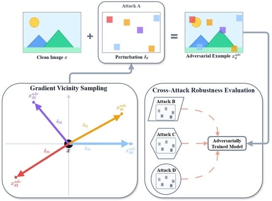
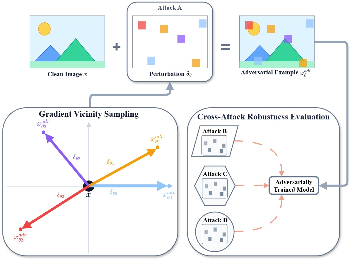
In this paper, we proposed the Gradient Vicinity Adversarial Training (GVAT). Under the $L_2$-norm constraint, perturbation directions were sampled in the vicinity of the gradient direction, with the sampling range bounded by a maximum angle. Unlike standard adversarial training, which generated adversarial examples along the original gradient direction, GVAT generated adversarial examples along the sampled perturbation directions and used them for adversarial training.

To evaluate the defense performance of GVAT, this paper applied GVAT to three attacks under the $L_2$-norm constraint: fast gradient sign method (FGSM) [16], projected gradient descent (PGD) [25], and Carlini–Wagner (CW) [26] under the $L_2$-norm constraint. FGSM was a single-step perturbation attack method based on the gradient direction. PGD was considered a multi-step perturbation attack method based on FGSM. CW was an optimization-based attack that minimized the perturbation magnitude by injecting perturbations into input images, while forcing misclassification.

To reduce training costs, we adopted an offline adversarial training setting, in which adversarial examples were generated in advance and then used for model training. Unlike prior offline methods that relied on multi-model transfer [27], our method used adversarial examples generated by only a single model. As a result, GVAT required only a single threat model setting during training and still improved the model’s transfer-based black-box robustness against other attacks, resulting in lower computational costs than methods that train with multiple attacks.

Experiments were conducted on three standard image classification datasets. MNIST [28] was a handwritten digit recognition task with 10 classes. CIFAR-10 and CIFAR-100 [29] were two natural image classification benchmarks with 10 and 100 classes.

The main contributions of this paper are summarized as follows:

• We propose Gradient Vicinity Adversarial Training, an adversarial training method that generated adversarial examples along directions sampled in the vicinity of the gradient direction.
• GVAT used adversarial examples generated by a single attack for training, but the trained models still show improved transfer-based black-box robustness against other attacks, including FGSM, PGD, sparse $L_1$ descent (SLIDE) [21], and CW attacks under the $L_1$, $L_2$, and $L_{\infty }$ constraints.
• We show that broader attack-direction coverage around the gradient direction was important for improving defense generalization, instead of relying only on stronger adversarial examples generated along the original gradient direction.

2. Methods

This section specified the threat model and the distance metric used to constrain the perturbation. We introduced the GVAT method. GVAT first sampled perturbation directions in the vicinity of the gradient. It then generated adversarial examples along the sampled directions and used them to train the model.

2.1. Threat Model

This paper primarily focused on transfer-based black-box robustness. The adversary was assumed to have access to the target network architecture, the input preprocessing pipeline, and the loss function, while the exact model parameters remained unknown. In this setting, the adversary trained a surrogate model using the known architecture, generated adversarial examples on the surrogate model, and then applied them directly to the target model. Prior studies had shown that adversarial examples generated on a surrogate model often transfer to the target model and retain nontrivial attack effectiveness [30].

This setting was distinct from white-box, in which adversarial examples were directly optimized using the gradients of the target model. Therefore, unless otherwise specified, the robustness and defense-generalization claims in this paper specifically referred to transfer-based black-box robustness. White-box robustness was evaluated separately using AutoAttack in an additional analysis.

Adversarial examples were generated using untargeted attacks, for which the objective was merely to cause misclassification. In contrast, targeted attacks had to drive the prediction to a specified target class. Since untargeted attacks had a less restrictive success criterion, they typically achieved higher success rates under the same perturbation budget, making the defense evaluation more challenging.

2.2. Distance Metric

To quantify the difference between adversarial examples and their corresponding original examples, prior studies have commonly adopted the $L_p$ distance as the metric, where $p\in \{1,2,\infty \}$. Specifically, for an original example x and its adversarial counterpart $x^{\prime }$, the $L_p$ distance was defined as ${\parallel x-x^{\prime }\parallel }_p$, where ${\parallel ·\parallel }_p$ was defined as follows:

$${\parallel \delta \parallel }_p={\left({\displaystyle \sum _{i=1}^n}{\left|{\delta }_i\right|}^p\right)}^{{\displaystyle \frac{1}{p}}}.$$

(1)

Specifically, the $L_1$-norm was often used to characterize sparse perturbations, the $L_{\infty }$-norm emphasized the maximum per-element deviation, and the $L_2$-norm reflected the overall perturbation energy and exhibited rotational symmetry.

The $L_2$-norm was used as the distance metric. During adversarial example generation and training, the perturbation magnitude was constrained by an $L_2$ ball, ensuring that adversarial examples always remained within the prescribed budget.

2.3. Gradient Vicinity Sampling

This section described how directions were sampled in the vicinity of the gradient during adversarial example generation in GVAT. Regardless of the specific attack formulation, the gradient considered here referred to the quantity used to guide the attack direction during adversarial example generation.

To confine sampled directions to the vicinity of the gradient direction, we imposed an angular constraint on the sampled direction relative to the original direction. Given the original gradient g, the new direction $v^{\prime }$ was sampled in the vicinity of g such that $\angle (v^{\prime },g)\le \theta$, where $\theta$ denoted the maximum sampling angle. The value of $\theta$ was manually specified to control the sampling range. In practice, the optimal $\theta$ might differ across attack methods.

In this paper, GVAT used adversarial examples generated by FGSM, PGD, and CW for adversarial training. For FGSM and PGD, original gradient g was computed as the gradient of the standard classification loss with respect to the perturbation. For CW, g was instead computed from the CW-specific objective.

The direction-sampling operation in the vicinity of the gradient direction was denoted by ${\mathrm{GV}}_{\theta }(·)$. To implement this sampling strategy, we sampled z from $z\sim \mathrm{Uniform}(\cos \theta ,1)$. The complete direction-sampling formulation was given as follows:

$$v^{\prime }={\mathrm{GV}}_{\theta }\left(g\right)=gz+u\sqrt{1-z^2}.$$

(2)

In Equation (2), u was a random unit vector satisfying $u^{\top }g=0$ and ${\parallel u\parallel }_2=1$. Therefore, the angle between ${\widehat{v}}^{\prime }$ and g was bounded by $\theta$. This ensured that the sampled direction remained within the prescribed angular vicinity of the original gradient direction.

Note that uniformly sampling z from $[\cos \theta ,1]$ did not result in a uniform distribution of the rotation angle. Let $\phi =\arccos \left(z\right)=\angle (g,{\mathbf{v}}^{\prime })$. By the change-of-variables rule, the induced angular density was

$$f_{\phi }\left(\phi \right)={\displaystyle \frac{\sin \phi }{1-\cos \theta }},0\le \phi \le \theta .$$

(3)

Therefore, the sampling strategy induced a non-uniform angular distribution proportional to $\sin \phi$. This was consistent with the design of GVAT, which only required the sampled direction to lie within the prescribed angular range $[0,\theta ]$, rather than to be uniformly distributed over the spherical cap.

2.4. Adversarial Example Generation in GVAT

This section described how adversarial examples were generated by sampling directions in the vicinity of the gradient. Given a normalized clean example $x_n$ with label y, gradient-vicinity direction sampling was performed at each gradient-based update. A single GVAT update was formulated as

$${\delta }^{\left(t\right)}=\left\{\begin{array}{cc}{\displaystyle {\mathrm{\Pi }}_{{\mathcal{B}}_2(0,ϵ)}\left({\delta }^{(t-1)}+\alpha {\mathrm{GV}}_{\theta }\left(g^{\left(t\right)}\right)\right),}\hfill & A\in \{\mathrm{FGSM},\mathrm{PGD}\},\hfill \\ {\displaystyle {\delta }^{(t-1)}-\eta {\mathrm{GV}}_{\theta }\left(g^{\left(t\right)}\right),}\hfill & A=\mathrm{CW}.\hfill \end{array}\right.$$

(4)

In Equation (4), A denoted the base attack type, ${\delta }^{\left(t\right)}$ denoted the perturbation after the t-th update, $\alpha$ denoted the update step size for FGSM and PGD, and $\eta$ denoted the optimization step size for CW. ${\mathrm{\Pi }}_{{\mathcal{B}}_2(0,ϵ)}$ denoted the projection onto the $L_2$ perturbation ball with radius $ϵ$, and $\theta$ denoted the maximum gradient-vicinity angle.

For FGSM-based GVAT, this update was performed once, whereas for PGD-based and CW-based GVAT, $g^{\left(t\right)}$ and the corresponding gradient-vicinity direction were recomputed at each iteration. The complete iterative procedures, including initialization, projection, and clipping, were provided in Algorithm 1. All attacks, perturbation budgets, and step sizes were defined in the normalized input space. The same perturbation budget was used for all channels. After the generation process, the adversarial inputs were de-normalized to the pixel space and clipped to the valid input range $[0,1]$.

Algorithm 1 Adversarial Example Generation in GVAT

Input: classifier $f_{\varphi }$; normalized input $x_n$ with label y; attack type A; iterations K; normalization mean $\mu$ and standard deviation $\sigma$; FGSM/PGD parameters $\alpha$ and $ϵ$; CW parameters $\eta$, and $\kappa$; maximum gradient-vicinity angle $\mathrm{\Theta }$. Output: adversarial example $x_n^{adv}$.   1: $l\leftarrow (0-\mu )/\sigma ,u\leftarrow (1-\mu )/\sigma$   2: if A is FGSM then   3:      $K\leftarrow 1$   4: end if   5: for $t=1$ to K do   6:      $x_n^{(t-1)}\leftarrow \mathrm{Clip}\left(x_n+{\delta }^{(t-1)},l,u\right)$   7:      if A is FGSM or PGD then   8:           ${\mathcal{L}}^{\left(t\right)}\leftarrow {\mathcal{L}}_{\mathrm{cls}}\left(f_{\varphi }\left(x_n^{(t-1)}\right),y\right)$   9:           $g^{\left(t\right)}\leftarrow {\nabla }_{\delta }{\mathcal{L}}^{\left(t\right)}$ 10:           $v^{\left(t\right)}\leftarrow G{V}_{\theta }\left(g^{\left(t\right)}\right)$ 11:           ${\delta }^{\left(t\right)}\leftarrow {\mathrm{\Pi }}_{{\mathcal{B}}_2(0,ϵ)}\left({\delta }^{(t-1)}+\alpha v^{\left(t\right)}\right)$ 12:      else if A is CW then 13:           ${\mathcal{L}}_{\mathrm{CW}}^{\left(t\right)}\leftarrow {\mathcal{L}}_{\mathrm{CW}}\left({\delta }^{(t-1)},x_n^{(t-1)},y,\kappa \right)$ 14:           $g^{\left(t\right)}\leftarrow {\nabla }_{\delta }{\mathcal{L}}_{\mathrm{CW}}^{\left(t\right)}$ 15:           $v^{\left(t\right)}\leftarrow G{V}_{\theta }\left(g^{\left(t\right)}\right)$ 16:           ${\delta }^{\left(t\right)}\leftarrow {\delta }^{(t-1)}-\eta v^{\left(t\right)}$ 17:      end if 18:      $x_n^{\left(t\right)}\leftarrow \mathrm{Clip}\left(x_n+{\delta }^{\left(t\right)},l,u\right)$ 19:      ${\delta }^{\left(t\right)}\leftarrow x_n^{\left(t\right)}-x_n$ 20: end for 21: $x_n^{adv}\leftarrow \mathrm{Clip}\left(x_n+{\delta }^{\left(K\right)},l,u\right)$ 22: return  $x_n^{adv}$

The adversarial examples used by GVAT during training were different from standard adversarial examples. Standard adversarial examples were generated along the gradient direction. In contrast, the adversarial examples used by GVAT were generated along directions sampled near the gradient direction. When the maximum sampling angle was set to $\theta =0$, GVAT reduced to the corresponding standard adversarial training method.

GVAT was considered only under the $L_2$-norm constraint. Under this constraint, the projection only rescaled the perturbation magnitude while preserving the sampled direction. In contrast, under $L_1$ and $L_{\infty }$ constraints, ${\mathrm{\Pi }}_{B_2(x,\epsilon )}$ corresponded to $L_1$-ball projection or element-wise clipping, which distorted the perturbation direction and weakened the controllability of the sampling angle.

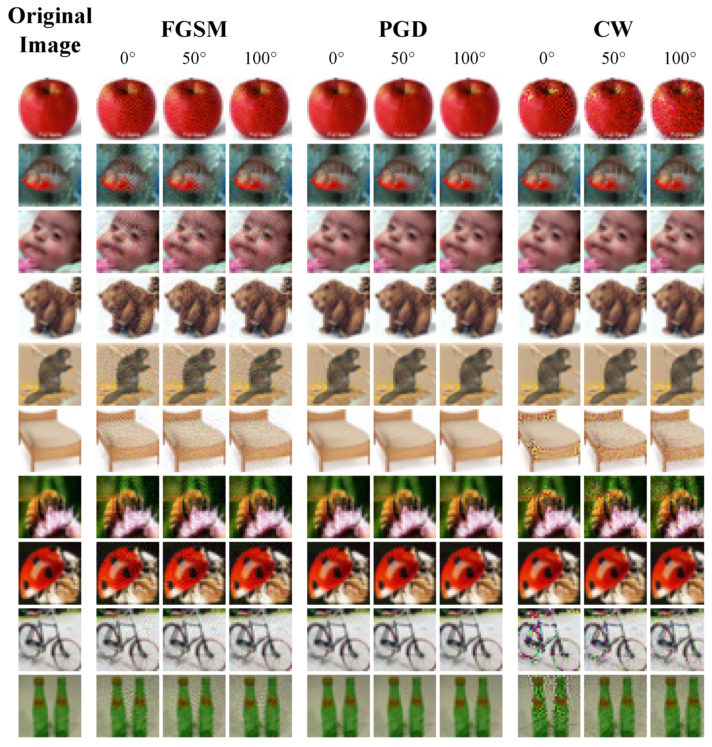
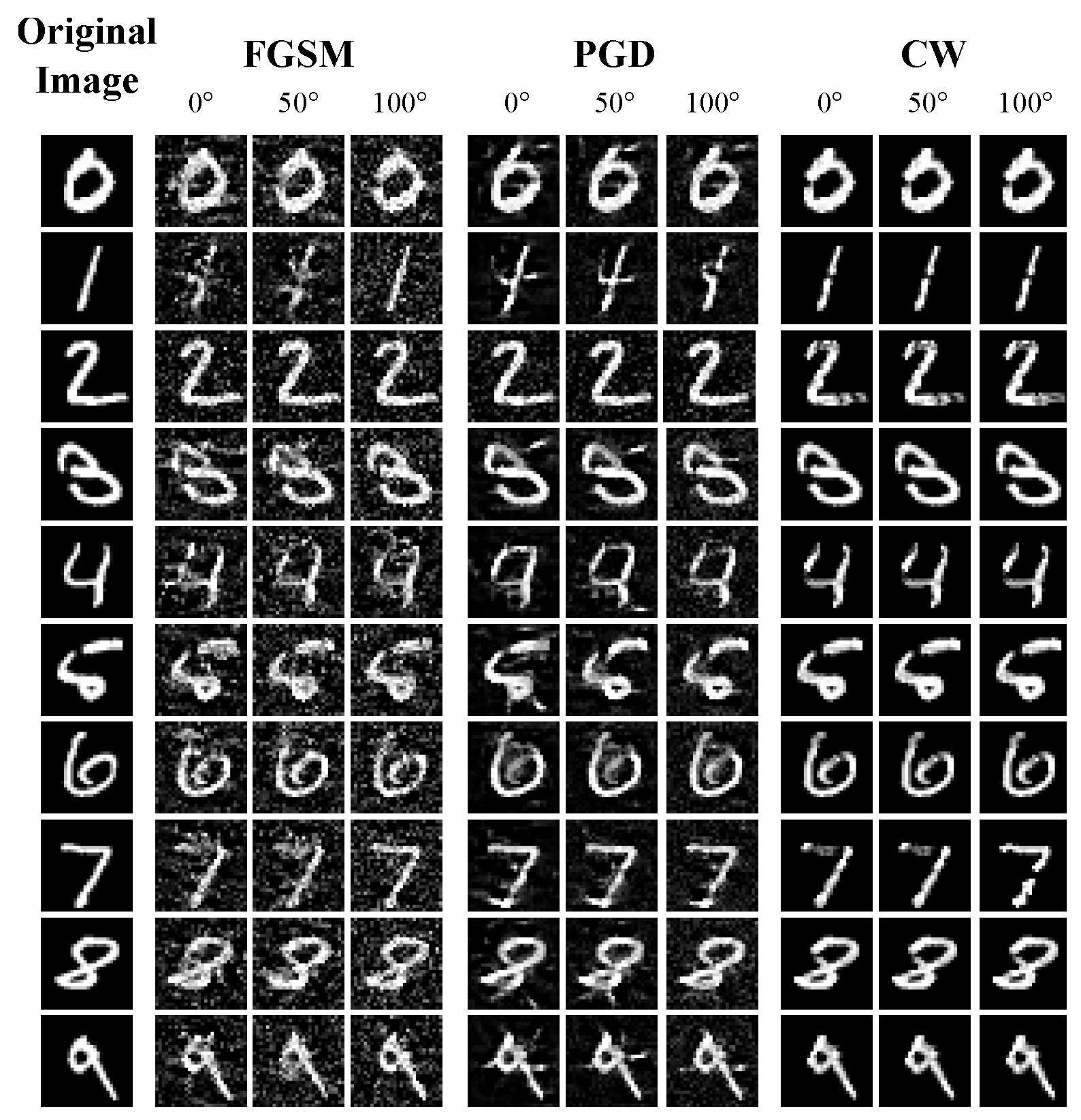
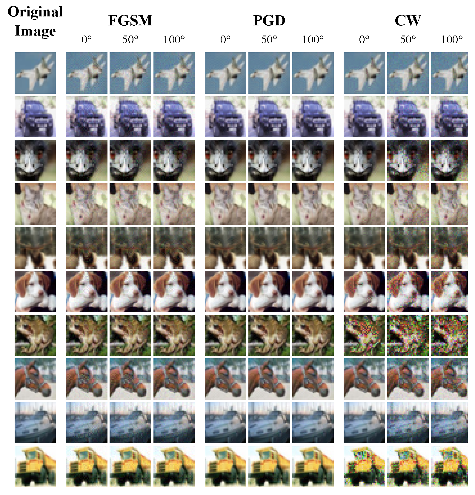
Figure 1 showed adversarial examples used in GVAT on CIFAR-100 with different maximum sampling angles $\theta =0^{°}$, ${50}^{°}$, and ${100}^{°}$. The corresponding visualizations for MNIST and CIFAR-10 were provided in Appendix A.

2.5. Datasets and Models

For the MNIST dataset, a lightweight CNN classifier was adopted, consisting of two convolutional layers, one fully connected layer, and an output layer. For data preprocessing, both training and testing inputs were converted to grayscale and then transformed into tensors, without additional normalization or data augmentation. The model was trained for 20 epochs using the Adam optimizer, with a learning rate of 0.001, ${\beta }_1=0.9$, $bet{a}_2=0.999$, $ϵ=1\times {10}^{-8}$, and no weight decay.

For the CIFAR-10 and CIFAR-100 datasets, WideResNet-28-10 [31] was used as the classifier. During training, data augmentation included random cropping to $32\times 32$ and random horizontal flipping. For CIFAR-100, Cutout regularization was additionally applied. The images were converted to tensors and normalized using the mean and standard deviation of each dataset. During testing, only tensor conversion and normalization were performed. The model was trained for 200 epochs using SGD with an initial learning rate of 0.1, momentum of 0.9, weight decay of $5\times {10}^{-4}$, and Nesterov momentum. A piecewise learning-rate schedule was adopted, where the learning rate was multiplied by 0.2, 0.2, and 0.5 at epochs 60, 120, and 160, respectively.

2.6. Adversarial Attack Settings

When selecting the adversarial attack parameters, we considered two aspects: the attack’s strength and the visual perceptibility of the perturbations.

Table 1. Experimental settings of adversarial attacks. The table reports the settings used on MNIST, CIFAR-10, and CIFAR-100, including the attack method, norm constraint, perturbation budget, step size, number of iterations, and whether GVAT was used. A checkmark indicates that GVAT was applied.

Dataset	Model	Attack Method	Distance Metric	Distance	Step Size	Iteration Steps	GVAT
MNIST	CNN	FGSM	$L_2$	6	1	1	✓
		FGSM	$L_{\infty }$	0.3	1	1
MNIST	CNN	PGD	$L_2$	4	2	40	✓
		PGD	$L_{\infty }$	0.15	0.1	40
		SLIDE	$L_1$	20	4	40
		CW	$L_2$	–	1	200	✓
CIFAR-10 & CIFAR-100	WideResNet -28-10	FGSM	$L_2$	6	1	1	✓
		FGSM	$L_{\infty }$	40/255	1	1
		PGD	$L_2$	4	2	10	✓
		PGD	$L_{\infty }$	40/255	2	10
		SLIDE	$L_1$	40	8	20
		CW	$L_2$	–	1	50	✓

summarized the various attack methods used in this paper and their corresponding perturbation budgets. SLIDE was a sparse adversarial attack under the $L_1$-norm constraint, which perturbs only a small number of pixels by following sparse gradient directions. SLIDE was used only as an attack method for evaluation.The confidence parameter was configured as 20 for MNIST, 1 for CIFAR-10, and 5 for CIFAR-100.

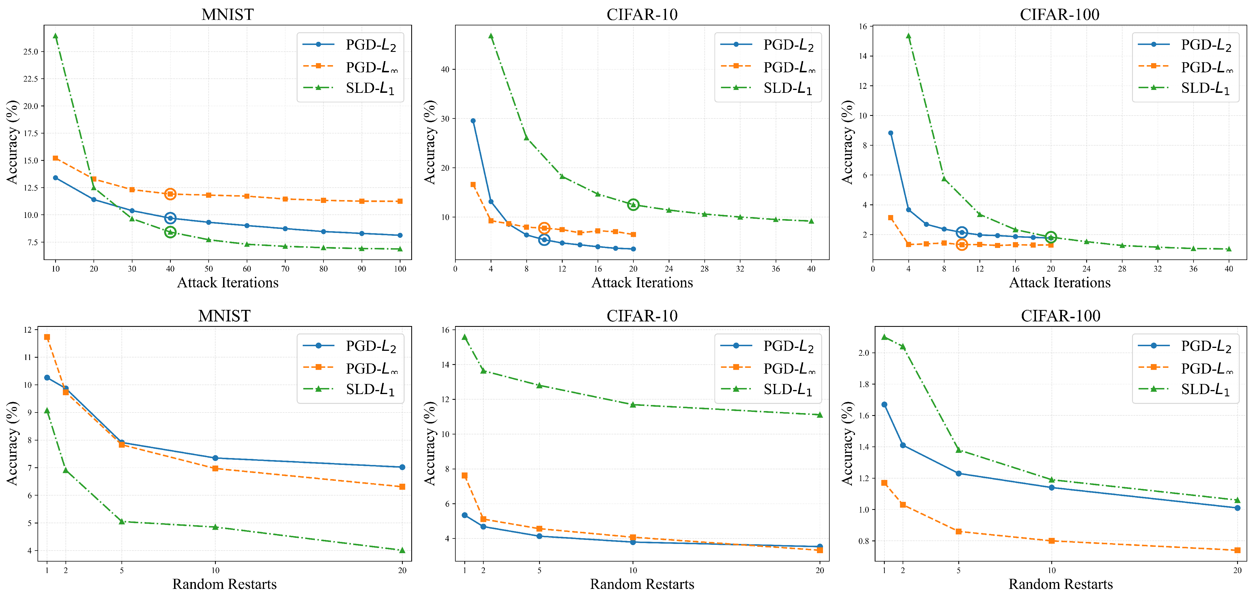
To assess the adequacy of the adopted attack settings, we further evaluated attack convergence on the source models used for adversarial-example generation by varying the number of attack iterations and random restarts. The attack performance gradually stabilized as the numbers of iterations and restarts increased, suggesting that further increases in these parameters had only limited effects on the attack results. Detailed results were provided in Appendix B.

2.7. Offline Adversarial Training and Testing

Unlike standard adversarial training, which dynamically generates adversarial examples for each training batch, we adopted offline adversarial training to reduce computational overhead. Under a fixed attack configuration, adversarial example sets for both the training and test sets were generated in advance using a surrogate model independently trained with the same architecture and training objective as the target model. During training, the original clean examples and their corresponding adversarial examples were concatenated along the batch dimension to form a combined input for parameter updates. During testing, Top-1 accuracy was evaluated on both the clean test set and adversarial example sets generated under different attack methods and norm constraints. These adversarial examples were generated on the surrogate model and then transferred to the target model; therefore, unless otherwise specified, the reported adversarial robustness refers to transfer-based black-box robustness.

Since no prior work had established the equivalence between offline and online adversarial training, we adopted the offline setting to enable large-scale comparative experiments at a controllable computational cost and to evaluate the effect of sampling directions in the vicinity of the gradient direction across different attack settings.

3. Results

This section presented the experimental results and analyzed the defense capability of standard adversarial training and GVAT under different attack settings, with particular emphasis on their performance against adversarial examples not used for training. Unless otherwise specified, the robustness results in the following transfer-based evaluations referred to transfer-based black-box robustness.

3.1. Standard Adversarial Training

We evaluated models trained with standard adversarial training against attacks with different methods and norm constraints.

Table 2. Classification Top-1 accuracy (%) of models trained with different adversarial examples. Rows represent training sets, and columns represent test sets. Clean denotes the original clean training or test set. Bold indicates the best result in each column.

Dataset	Training Set	Testing Set
		Clean	FGSM, ${\mathit{L}}_{\mathbf{2}}$	FGSM, ${\mathit{L}}_{\infty }$	PGD, ${\mathit{L}}_{\mathbf{2}}$	PGD, ${\mathit{L}}_{\infty }$	SLIDE, ${\mathit{L}}_{\mathbf{1}}$	CW, ${\mathit{L}}_{\mathbf{2}}$
MNIST	Clean	99.22	39.38	47.65	17.17	82.85	49.04	32.11
	FGSM, $L_2$	98.92	98.35	96.54	83.40	98.86	82.64	75.50
	FGSM, $L_{\infty }$	99.01	86.65	98.54	62.33	98.35	76.94	67.85
	PGD, $L_2$	98.94	87.87	76.17	98.77	98.46	84.53	76.65
	PGD, $L_{\infty }$	99.12	84.39	92.02	67.71	99.16	70.94	58.29
	SLIDE, $L_1$	98.60	86.64	80.27	96.76	97.52	98.05	88.49
	CW, $L_2$	98.05	72.71	62.93	78.81	90.68	87.49	96.69
CIFAR-10	Clean	94.44	33.89	33.38	24.98	22.62	44.10	47.59
	FGSM, $L_2$	93.89	92.40	82.69	65.29	77.45	75.34	63.80
	FGSM, $L_{\infty }$	94.08	73.01	87.47	61.12	83.59	70.23	67.43
	PGD, $L_2$	93.94	72.42	61.52	94.78	65.81	91.48	65.77
	PGD, $L_{\infty }$	91.32	68.85	68.52	82.25	86.47	83.81	74.94
	SLIDE, $L_1$	93.92	76.10	69.60	84.80	77.37	92.77	71.73
	CW, $L_2$	93.66	71.62	63.81	88.98	72.39	89.64	92.42
CIFAR-100	Clean	76.57	5.78	5.73	16.38	4.45	25.96	24.35
	FGSM, $L_2$	73.34	56.91	50.06	49.06	58.75	55.71	48.51
	FGSM, $L_{\infty }$	74.58	41.19	61.35	42.51	66.55	49.70	34.70
	PGD, $L_2$	74.53	28.99	19.38	69.06	19.40	64.42	40.13
	PGD, $L_{\infty }$	73.71	37.07	43.10	52.76	67.49	56.19	46.20
	SLIDE, $L_1$	74.69	37.37	23.10	59.66	35.83	66.81	46.63
	CW, $L_2$	73.68	31.31	22.48	59.99	25.83	64.57	70.79

shows the Top-1 accuracy on MNIST, CIFAR-10, and CIFAR-100. Models were trained on different adversarial examples using standard adversarial training and evaluated under different test attacks. We found that the defense performance decreased when the training attack differed from the test attack. This occurred for both different attack types and different norm constraints.

• Different attack types. The defense performance decreased when the test attack differed from the training attack. For example, on CIFAR-100, the model trained with FGSM, $L_2$ achieved 56.91% Top-1 accuracy under the same attack, but only 48.51% under the CW, $L_2$ attack. Similar trends were observed on CIFAR-10 as well.
• Different norm constraints. The defense performance also decreased when the test norm differed from the training norm. For example, on CIFAR-100, the model trained with PGD, $L_2$ adversarial examples achieved 69.06% Top-1 accuracy under the same $L_2$ setting. However, its accuracy dropped to 19.40% under the PGD, $L_{\infty }$ attack. Similar trends were also observed on other datasets.

These results indicated that the defense learned from offline adversarial training was strongly tied to the specific attack algorithm and norm constraint used during training. To generalize the defense effect learned from one attack to other attacks, GVAT was introduced.

3.2. Gradient Vicinity Adversarial Training

We evaluated the defense ability of GVAT under different adversarial examples.

Table 3. Classification Top-1 accuracy (%) of models trained with GVAT adversarial examples under different training sets and maximum sampling angles $\theta$. The setting $\theta =0^{°}$ denotes adversarial training using the original attack direction, while larger angles denote GVAT with directions sampled within the corresponding maximum angular range. Bold indicates the best result in each column.

Dataset	Training Set	GVAT $\mathit{\theta }$	Testing Set
			Clean	FGSM ${\mathit{L}}_{\mathbf{2}}$	FGSM ${\mathit{L}}_{\infty }$	PGD ${\mathit{L}}_{\mathbf{2}}$	PGD ${\mathit{L}}_{\infty }$	SLIDE ${\mathit{L}}_{\mathbf{1}}$	CW ${\mathit{L}}_{\mathbf{2}}$
MNIST	FGSM, $L_2$	$0^{°}$	98.92	98.35	96.54	83.40	98.86	82.64	75.50
		${25}^{°}$	98.97	98.30	97.33	83.04	98.79	82.20	71.36
		${50}^{°}$	98.83	97.28	96.46	76.90	98.67	80.22	70.23
		${100}^{°}$	98.74	95.54	97.14	83.40	98.57	88.27	76.72
		${120}^{°}$	98.90	94.80	96.76	81.70	98.39	88.58	74.92
		${150}^{°}$	98.92	91.70	95.54	75.65	97.88	87.20	76.70
MNIST	PGD, $L_2$	$0^{°}$	98.94	87.87	76.17	98.77	98.46	84.53	76.65
		${25}^{°}$	99.07	87.46	77.45	98.66	98.32	85.88	76.55
		${50}^{°}$	98.94	90.85	82.94	98.58	98.86	84.22	73.83
		${100}^{°}$	98.90	91.70	87.10	97.39	99.15	86.66	77.25
		${120}^{°}$	98.98	95.14	95.74	95.75	99.21	92.92	84.13
		${150}^{°}$	98.92	91.70	95.54	75.65	97.88	87.20	73.72
MNIST	CW, $L_2$	$0^{°}$	98.05	72.71	62.93	78.81	90.68	87.49	96.69
		${25}^{°}$	98.17	76.79	72.48	80.85	93.47	86.54	95.55
		${50}^{°}$	98.07	75.12	72.91	79.28	92.34	86.39	95.67
		${100}^{°}$	97.88	78.22	76.88	80.92	93.18	86.03	94.79
		${120}^{°}$	97.95	79.60	79.96	83.49	93.44	87.37	95.66
		${150}^{°}$	97.90	82.30	86.22	76.73	95.67	85.55	91.25
CIFAR-10	FGSM, $L_2$	$0^{°}$	93.89	92.00	82.69	65.29	77.45	75.34	63.80
		${25}^{°}$	94.10	89.56	81.77	66.58	81.71	76.39	66.48
		${50}^{°}$	94.23	92.18	85.95	72.58	83.49	80.31	67.62
		${100}^{°}$	93.41	84.98	82.28	91.33	90.34	91.50	82.36
		${120}^{°}$	94.16	83.48	80.76	90.39	89.08	90.87	81.03
		${150}^{°}$	93.95	81.89	79.18	89.47	88.79	89.99	76.45
CIFAR-10	PGD, $L_2$	$0^{°}$	93.94	72.42	61.52	94.78	65.81	91.48	65.77
		${25}^{°}$	93.20	67.22	58.83	91.36	60.16	88.98	57.26
		${50}^{°}$	93.56	70.89	61.25	90.11	64.30	89.63	58.37
		${100}^{°}$	93.62	76.33	68.57	91.73	74.16	90.69	66.95
		${120}^{°}$	94.14	74.33	66.36	90.88	76.97	90.54	76.69
		${150}^{°}$	93.35	62.42	58.06	85.93	70.56	87.12	73.69
CIFAR-10	CW, $L_2$	$0^{°}$	93.66	71.62	63.81	88.98	72.39	89.64	92.42
		${25}^{°}$	94.22	80.57	75.81	90.08	87.22	91.14	92.81
		${50}^{°}$	93.82	79.01	76.04	89.24	87.66	90.21	90.71
		${100}^{°}$	94.41	72.02	71.12	85.29	88.49	87.80	87.48
		${120}^{°}$	94.13	70.23	69.58	84.07	87.75	87.21	86.78
		${150}^{°}$	94.21	72.90	71.82	85.38	88.25	87.84	88.37
CIFAR-100	FGSM, $L_2$	$0^{°}$	73.34	56.91	50.06	49.06	58.75	55.71	48.51
		${25}^{°}$	74.24	60.21	51.82	48.78	60.98	56.74	52.12
		${50}^{°}$	73.19	58.08	49.32	55.70	60.16	60.05	52.94
		${100}^{°}$	73.25	59.21	52.91	60.38	65.16	62.81	56.13
		${120}^{°}$	74.13	55.87	49.73	58.51	66.01	61.51	56.54
		${150}^{°}$	74.27	56.97	50.94	57.58	65.24	62.11	57.92
CIFAR-100	PGD, $L_2$	$0^{°}$	74.53	28.99	19.38	69.06	19.40	64.42	40.13
		${25}^{°}$	73.75	28.89	18.41	65.14	21.99	64.43	39.12
		${50}^{°}$	73.66	40.67	26.23	66.07	32.11	66.40	41.73
		${100}^{°}$	74.12	46.12	33.79	64.54	42.98	66.06	48.21
		${120}^{°}$	74.75	41.36	28.90	61.48	40.22	64.68	49.97
		${150}^{°}$	74.17	33.08	24.10	54.68	36.61	59.81	46.82
CIFAR-100	CW, $L_2$	$0^{°}$	73.68	31.31	22.48	59.99	25.83	64.57	70.79
		${25}^{°}$	75.04	50.66	40.40	62.00	55.14	66.32	70.00
		${50}^{°}$	74.95	52.64	42.73	59.14	59.85	63.93	67.45
		${100}^{°}$	74.19	39.02	32.51	49.03	56.08	56.79	59.16
		${120}^{°}$	73.18	36.75	30.03	46.84	53.89	55.80	58.32
		${150}^{°}$	75.03	43.76	36.07	50.35	61.21	58.69	61.64

reports the accuracy of models trained by GVAT. During training, adversarial examples were generated by using FGSM, PGD, and CW with different maximum sampling angles $\theta$.

As mentioned in the Section 2.3, $\theta$ controlled the maximum angular deviation between the sampled direction and the original gradient direction.

• Different attack types and norm constraints. GVAT improved defense performance on many adversarial examples not used for training. This indicated that GVAT could improve the generalization of defense effects. For example, on CIFAR-100, compared with standard PGD, $L_2$ adversarial training, PGD, $L_2$-based GVAT with $\theta ={100}^{°}$ increased the Top-1 accuracy under the FGSM, $L_2$ attack from 28.99% to 46.12%.
• Larger angle was not always better. A larger maximum sampling angle did not always lead to better defense performance. In some cases, the accuracy first increased and then decreased as $\theta$ became larger. For example, on CIFAR-100, when GVAT was applied to PGD, $L_2$, the best performance under the FGSM, $L_2$ test attack appeared at $\theta ={100}^{°}$, rather than at the largest angle.

GVAT achieved higher Top-1 accuracy than standard adversarial training on most adversarial examples not used for training. As the sampling range increased, the accuracy under these attacks first rose, then fell. At some rotation angles, the accuracy against the training attacks decreased slightly. However, it was still higher than that of the model trained without adversarial training.

3.3. Comparison with Multi-Attack Defense Methods

Multi-attack defense methods used multiple attacks or perturbation norms during training. Their goal was to improve robustness against multiple attacks. In contrast, GVAT used only one base attack.

Therefore, we compared GVAT with standard adversarial training (AT), multi-attack training (Multi-AT) [21], and Multi-Steepest Descent (MSD) [32]. Multi-AT used multiple attack types, while MSD jointly considered multiple perturbation norms during adversarial optimization. We evaluated these methods in terms of computational cost and transfer-based black-box robustness.

1.

Computational cost. As shown in

Table 4. Computational cost comparison of different adversarial training methods on CIFAR-100. This table reported the computational cost in terms of gradient evaluations, adversarial-example generation time, training time, total GPU time, and storage overhead.

Method	Attack Setting	Grad. Evals. /Sample	Adv. Gen. Time (h)	Training Time (h)	GPU Time (h)	Storage (GB)
Multi-AT	PGD, $L_2$ PGD $L_{\infty }$ CW, $L_2$	920	2.85	13.43	16.28	2.57
MSD	PGD over $L_1,L_2,L_{\infty }$	30	0.90	10.35	11.25	0.85
AT	FGSM, $L_2$	1	0.24	10.37	10.61	0.85
GVAT	FGSM, $L_2$	1	0.24	10.43	10.67	0.85

, Multi-AT had the highest cost, with 920 gradient evaluations per sample, 16.28 h of total GPU time, and 2.57 GB of storage. MSD required 30 gradient evaluations per sample and 11.25 h of total GPU time. AT and GVAT had similar computational costs, with total GPU times of 10.61 h and 10.67 h, respectively.

2.

Transfer-based black-box robustness.

Table 5. Top-1 Classification Accuracy (%) of Multi-Attack Defense Methods on MNIST, CIFAR-10, and CIFAR-100. Bold indicates the best result in each column.

Dataset	Method	Testing Set						Avg.
		FGSM, ${\mathit{L}}_{\mathbf{2}}$	FGSM, ${\mathit{L}}_{\infty }$	PGD, ${\mathit{L}}_{\mathbf{2}}$	PGD, ${\mathit{L}}_{\infty }$	SLIDE, ${\mathit{L}}_{\mathbf{1}}$	CW, ${\mathit{L}}_{\mathbf{2}}$
MNIST	Multi-AT	94.09	90.85	99.17	99.37	96.60	98.01	96.35
	MSD	81.26	68.08	97.41	96.87	84.42	78.16	84.36
	AT	98.35	96.54	83.40	98.86	82.64	75.50	89.22
	GVAT	95.54	97.14	83.40	98.57	88.27	76.72	89.94
CIFAR-10	Multi-AT	87.20	80.92	93.01	92.62	93.06	93.45	90.04
	MSD	83.06	80.54	91.20	91.12	91.04	77.58	85.75
	AT	92.00	82.69	65.29	77.45	75.34	63.80	76.10
	GVAT	84.98	82.28	91.33	90.34	91.50	82.36	87.13
CIFAR-100	Multi-AT	60.30	61.99	71.36	76.52	74.58	78.00	70.46
	MSD	54.92	50.97	63.41	67.86	64.84	58.34	60.05
	AT	56.91	50.06	49.06	58.75	55.71	48.51	53.17
	GVAT	59.21	52.91	60.38	65.16	62.81	56.13	59.43

compared AT, GVAT, Multi-AT, and MSD against six adversarial attacks. Multi-AT achieved the highest average robust accuracy on all three datasets. GVAT ranked second on MNIST and CIFAR-10. On CIFAR-100, its average robust accuracy was 59.43%, which was close to the 60.05% achieved by MSD. GVAT achieved higher average robust accuracy than AT.

Overall, GVAT achieved lower robustness than Multi-AT, but higher robustness than conventional single-attack AT while relying on only one base attack for training. GVAT also incurred lower computational cost than Multi-AT.

3.4. White-Box Robustness Evaluation with AutoAttack

GVAT was designed under the transfer-based black-box threat model defined in Section 2.1, where adversarial examples were generated on an independently trained surrogate model and then transferred to the target model. To further investigate the effectiveness of GVAT under a stronger white-box setting, we conducted a direct white-box evaluation on the target models using AutoAttack [33].

Table 6. White-box robustness evaluation using AutoAttack on MNIST, CIFAR-10, and CIFAR-100. The reported values are Top-1 classification accuracy (%) under APGD-CE, APGD-DLR, FAB-T, Square Attack, and the standard AutoAttack ensemble. Bold indicates the best result in each column.

Dataset	Training Set	GVAT $\mathit{\theta }$	Testing Set
			APGD-CE	APGD-DLR	FAB-T	SQUARE	STANDARD
MNIST	FGSM, $L_2$	$0^{°}$	34.25	0.33	7.85	7.05	0.04
		${25}^{°}$	24.18	0.11	8.86	4.83	0.02
		${50}^{°}$	7.46	0.98	8.07	9.74	0.17
		${100}^{°}$	5.42	1.67	8.53	10.73	0.42
		${120}^{°}$	35.30	3.43	10.70	15.98	1.14
		${150}^{°}$	49.18	10.91	15.58	27.53	7.12
	PGD, $L_2$	$0^{°}$	14.26	0.00	11.90	0.17	0.00
		${25}^{°}$	0.59	0.00	7.66	0.20	0.00
		${50}^{°}$	11.70	0.00	9.15	0.13	0.00
		${100}^{°}$	1.17	0.00	8.35	1.40	0.00
		${120}^{°}$	15.51	0.14	10.90	3.25	0.01
		${150}^{°}$	38.78	41.22	44.75	55.15	37.82
	CW, $L_2$	$0^{°}$	1.41	0.01	13.18	0.22	0.00
		${25}^{°}$	0.54	0.06	12.54	0.65	0.00
		${50}^{°}$	1.52	0.03	13.97	0.35	0.00
		${100}^{°}$	0.88	0.02	11.71	0.96	0.01
		${120}^{°}$	1.50	0.05	15.45	0.61	0.00
		${150}^{°}$	4.33	4.90	11.04	11.93	3.08
CIFAR-10	FGSM, $L_2$	$0^{°}$	0.01	0.07	0.16	18.34	0.00
		${25}^{°}$	0.03	0.20	0.09	26.86	0.00
		${50}^{°}$	0.13	0.21	0.15	29.54	0.00
		${100}^{°}$	2.94	6.30	1.40	44.61	0.85
		${120}^{°}$	4.65	10.73	3.41	49.60	2.64
		${150}^{°}$	4.38	11.24	3.32	49.18	2.39
	PGD, $L_2$	$0^{°}$	0.00	0.00	0.53	3.24	0.00
		${25}^{°}$	0.00	0.00	0.31	9.43	0.00
		${50}^{°}$	0.00	0.01	0.14	12.20	0.00
		${100}^{°}$	0.02	0.04	0.24	11.36	0.00
		${120}^{°}$	0.00	0.00	0.22	11.55	0.00
		${150}^{°}$	0.23	0.86	0.23	28.18	0.08
	CW, $L_2$	$0^{°}$	0.09	0.29	0.17	19.17	0.00
		${25}^{°}$	0.32	0.77	0.51	26.74	0.14
		${50}^{°}$	4.18	9.61	2.98	46.67	2.41
		${100}^{°}$	12.28	23.01	10.75	56.03	9.52
		${120}^{°}$	12.20	18.95	9.63	54.33	8.45
		${150}^{°}$	12.67	21.06	11.32	55.14	10.06
CIFAR-100	FGSM, $L_2$	$0^{°}$	1.55	1.67	1.51	24.78	0.89
		${25}^{°}$	1.62	1.40	1.29	25.12	0.80
		${50}^{°}$	1.23	1.26	1.19	25.36	0.69
		${100}^{°}$	2.36	2.87	2.65	26.43	1.70
		${120}^{°}$	2.20	2.30	1.98	25.85	1.44
		${150}^{°}$	2.02	2.50	1.90	26.21	1.46
	PGD, $L_2$	$0^{°}$	0.03	0.02	0.37	4.31	0.00
		${25}^{°}$	0.12	0.09	0.32	7.25	0.03
		${50}^{°}$	0.04	0.04	0.34	8.59	0.00
		${100}^{°}$	0.25	0.24	0.52	14.35	0.09
		${120}^{°}$	0.31	0.25	0.51	16.64	0.08
		${150}^{°}$	0.49	0.60	0.76	17.42	0.22
	CW, $L_2$	$0^{°}$	0.07	0.05	0.28	7.30	0.01
		${25}^{°}$	0.46	0.44	0.69	17.73	0.20
		${50}^{°}$	1.53	1.73	1.52	23.91	0.94
		${100}^{°}$	1.91	1.87	1.68	24.54	1.19
		${120}^{°}$	1.60	1.72	1.39	23.42	1.06
		${150}^{°}$	2.02	1.77	1.47	23.62	1.11

reported the white-box robustness of models trained with different GVAT configurations under APGD-CE, APGD-DLR, FAB-T, Square Attack, and standard AutoAttack.

On MNIST, GVAT showed clear improvements at larger gradient-vicinity angles. For example, PGD, $L_2$-based GVAT with $\theta ={150}^{°}$ reached 37.82% standard AutoAttack accuracy. On CIFAR-10, CW, $L_2$-based GVAT showed the most notable improvement. The standard AutoAttack accuracy increased from 0.00% to 10.06% at $\theta ={150}^{°}$.

Although the defense effects learned by GVAT could generalize to some extent beyond the original transfer-based setting, its white-box robustness remained limited. This limitation may have been partly related to the offline training procedure, where adversarial examples were pre-generated on a surrogate model and were not updated according to the evolving target model during training. The primary objective of GVAT remained to improve the generalization of defense effects learned from a single adversarial attack under the transfer-based black-box threat model defined in Section 2.1.

4. Discussion

In the GVAT method, adversarial examples generated by FGSM and PGD generally had lower attack strength. Despite this, the models trained with GVAT were stronger at defending against adversarial examples under the transfer-based black-box setting. They performed better on examples that were not used during training.

This observation was inconsistent with the view that stronger attacks used in adversarial training led to better defense capability. We argued that broader coverage of attack directions was more important than attack strength in defending against adversarial attacks.

4.1. Effect of Attack Strength on Defense Performance

We observed two different effects of attack strength. Simply reducing the attack strength by adjusting the $L_2$ perturbation magnitude weakened the effectiveness of adversarial training. In contrast, adversarial examples used by GVAT could still improve defense performance after the maximum sampling angle was properly adjusted. This occurred even when these adversarial examples had lower attack strength.

To evaluate how attack strength affected defense performance, we conducted a controlled experiment on CIFAR-100 by adjusting the $L_2$ perturbation magnitude of the training adversarial examples while keeping the original attack direction unchanged. Attack strength was measured by classification accuracy on the baseline model, with lower accuracy indicating a stronger attack.

Table 7. Classification Top-1 accuracy (%) on CIFAR-100 for models trained with $L_2$-adjusted FGSM or PGD adversarial examples at different attack strengths. The third column reports the Top-1 accuracy used to indicate the strength of the corresponding training adversarial examples. Bold indicates the best result in each column.

Dataset	Training Set	Accuracy	Testing Set
			Clean	FGSM ${\mathit{L}}_{\mathbf{2}}$	FGSM ${\mathit{L}}_{\infty }$	PGD ${\mathit{L}}_{\mathbf{2}}$	PGD ${\mathit{L}}_{\infty }$	SLIDE ${\mathit{L}}_{\mathbf{1}}$	CW ${\mathit{L}}_{\mathbf{2}}$
CIFAR-100	PGD, $L_2$	2.23	73.77	23.48	16.15	66.61	16.81	61.44	38.69
		10.29	74.85	19.01	12.36	65.67	13.65	62.27	38.53
		50.32	74.82	11.81	9.65	40.09	12.05	48.71	36.82
	FGSM, $L_2$	2.58	73.34	56.91	50.06	49.06	58.75	55.71	48.51
		15.11	73.41	55.69	39.36	59.76	41.81	63.53	41.67
		37.43	73.34	19.33	13.56	57.93	16.50	59.64	37.16

reports the results on CIFAR-100. The models were trained with $L_2$-adjusted PGD or FGSM adversarial examples. Different Top-1 accuracy values in the third column indicate different attack strengths of the training adversarial examples. The results showed that, when the attack strength was reduced, the defense performance of the resulting model generally declined.

To examine the attack strength of adversarial examples generated by GVAT under different maximum sampling angles $\theta$. The attack strength was evaluated by measuring its effect on a baseline model trained on the standard clean CIFAR-100 training set.

Table 8. Top-1 accuracy (%) on CIFAR-100 under adversarial examples generated using different maximum sampling angles $\theta$. The model was trained only on clean examples. Lower accuracy indicates stronger attack strength.

GVAT $\mathit{\theta }$	FGSM ${\mathit{L}}_2$	PGD ${\mathit{L}}_2$	CW ${\mathit{L}}_2$
$0^{°}$	5.78	16.38	24.35
${25}^{°}$	5.94	17.30	22.58
${50}^{°}$	6.91	19.43	17.47
${100}^{°}$	18.35	34.57	10.65
${120}^{°}$	26.89	47.27	10.12
${150}^{°}$	32.41	59.38	10.98

reports the Top-1 accuracy of the baseline model under these adversarial examples. As $\theta$ increased, the accuracy under FGSM and PGD generally increased. In contrast, the accuracy under CW decreased when $\theta$ increased from $0^{°}$ to ${120}^{°}$. This was because the gradient direction was the locally most effective attack direction, and deviating from it tended to weaken the attack. However, the model trained with GVAT still performed better on most adversarial examples not used for training.

4.2. Effect of Attack Direction Coverage on Defense Performance

To evaluate the effect of attack direction coverage on defense performance, we compared two adversarial training methods. The first method was GVAT with different maximum sampling angles. The second method was $L_2$-adjusted adversarial training along the original gradient direction. In the second method, only the magnitude of the $L_2$ perturbation was adjusted. This made its attack strength close to that of GVAT.

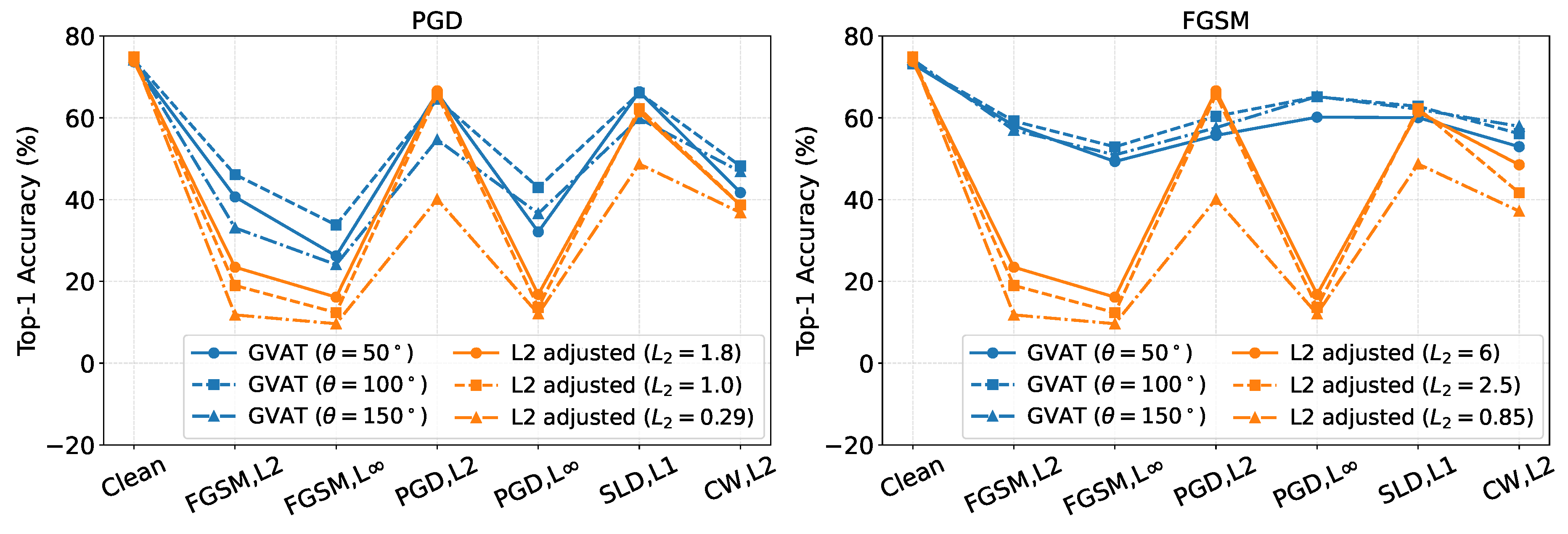
The results of the two comparative experiments above were shown in Figure 2. Models trained with GVAT tended to perform better on most adversarial examples not used for training than those trained with matched-strength adversarial examples.

One possible explanation was that GVAT increased the diversity of attack directions covered during training. By sampling directions in the vicinity of the gradient, adversarial examples could be generated along multiple attack directions rather than a single attack trajectory. As a result, the model was exposed to a broader range of adversarial variations during training. This broader attack direction coverage might be more important than attack strength itself for improving defense performance. In contrast, CW tended to become stronger as $\theta$ increased, since it sought perturbations that both induced misclassification and remained small in magnitude. Thus, deviating from the original direction might have helped CW find stronger directions beyond it.

5. Conclusions

In this work, we proposed Gradient Vicinity Adversarial Training (GVAT), which generated adversarial examples along directions sampled in the vicinity of the gradient. The goal of GVAT was to generalize the defense effect from one specific attack to other attacks under the transfer-based black-box setting. The results showed that GVAT not only defended against the corresponding attacks that generated adversarial examples but also defended against other attacks. In other words, the defense effect of GVAT was generalized to other attacks under the transfer-based black-box setting.

References

1. Zhu, L.; Liao, B.; Zhang, Q.; Wang, X.; Liu, W.; Wang, X. Vision Mamba: Efficient visual representation learning with bidirectional state space model. In Proceedings of the 41st International Conference on Machine Learning, Vienna, Austria, 21–27 July 2024; pp. 62429–62442. Available online: https://proceedings.mlr.press/v235/zhu24f.html (accessed on 6 September 2026).
2. Radford, A.; Kim, J.W.; Hallacy, C.; Ramesh, A.; Goh, G.; Agarwal, S.; Sastry, G.; Askell, A.; Mishkin, P.; Clark, J.; et al. Learning transferable visual models from natural language supervision. In Proceedings of the 38th International Conference on Machine Learning, Virtual Event, 18–24 July 2021; pp. 8748–8763. Available online: https://proceedings.mlr.press/v139/radford21a.html (accessed on 6 September 2026).
3. Li, Z.; Wang, W.; Li, H.; Xie, E.; Sima, C.; Lu, T.; Qiao, Y.; Dai, J. BEVFormer: Learning bird’s-eye-view representation from LiDAR-camera via spatiotemporal transformers. IEEE Trans. Pattern Anal. Mach. Intell. 2025, 47, 2020–2036. [Google Scholar] [CrossRef] [Scilit] [PubMed]
4. Hu, Y.; Yang, J.; Chen, L.; Li, K.; Sima, C.; Zhu, X.; Chai, S.; Du, S.; Lin, T.; Wang, W.; et al. Planning-oriented autonomous driving. In Proceedings of the IEEE/CVF Conference on Computer Vision and Pattern Recognition (CVPR 2023), Vancouver, BC, Canada, 17–24 June 2023; pp. 17853–17862. [Google Scholar] [CrossRef] [Scilit]
5. Hinton, G.; Deng, L.; Yu, D.; Dahl, G.E.; Mohamed, A.R.; Jaitly, N.; Senior, A.; Vanhoucke, V.; Nguyen, P.; Sainath, T.N.; et al. Deep Neural Networks for Acoustic Modeling in Speech Recognition. IEEE Signal Process. Mag. 2012, 29, 82–97. [Google Scholar] [CrossRef] [Scilit]
6. Radford, A.; Kim, J.W.; Xu, T.; Brockman, G.; McLeavey, C.; Sutskever, I. Robust speech recognition via large-scale weak supervision. In Proceedings of the International Conference on Machine Learning (ICML 2023), Honolulu, HI, USA, 23–29 July 2023; pp. 28492–28518. Available online: https://proceedings.mlr.press/v202/radford23a.html (accessed on 6 September 2026).
7. Szegedy, C.; Zaremba, W.; Sutskever, I.; Bruna, J.; Erhan, D.; Goodfellow, I.J.; Fergus, R. Intriguing properties of neural networks. In Proceedings of the 2nd International Conference on Learning Representations (ICLR 2014), Banff, AB, Canada, 14–16 April 2014. [Google Scholar] [CrossRef] [Scilit]
8. Biggio, B.; Roli, F. Wild Patterns: Ten Years After the Rise of Adversarial Machine Learning. In Proceedings of the 2018 ACM SIGSAC Conference on Computer and Communications Security, Toronto, ON, Canada, 15–19 October 2018. [Google Scholar] [CrossRef] [Scilit]
9. Wang, L.; Zhang, T.; Han, Y.; Fang, M.; Jin, T.; Kang, J. Attack end-to-end autonomous driving through module-wise noise. In Proceedings of the IEEE/CVF Conference on Computer Vision and Pattern Recognition Workshops, Seattle, WA, USA, 17–18 June 2024; pp. 8349–8352. Available online: https://openaccess.thecvf.com/content/CVPR2024W/AdvML/html/Wang_Attack_End-to-End_Autonomous_Driving_through_Module-Wise_Noise_CVPRW_2024_paper.html (accessed on 6 September 2026).
10. Carlini, N.; Mishra, P.; Vaidya, T.; Zhang, Y.; Sherr, M.; Shields, C.; Wagner, D.A.; Zhou, W. Hidden voice commands. In Proceedings of the 25th USENIX Security Symposium (USENIX Security 16), Austin, TX, USA, 10–12 August 2016; pp. 513–530. Available online: https://www.usenix.org/conference/usenixsecurity16/technical-sessions/presentation/carlini (accessed on 6 September 2026).
11. Zuo, F.; Zeng, Q. Exploiting the sensitivity of L2 adversarial examples to erase-and-restore. In Proceedings of the 2021 ACM Asia Conference on Computer and Communications Security, Virtual Event, 7–11 June 2021; pp. 40–51. [Google Scholar] [CrossRef] [Scilit]
12. Li, X.; Li, F. Adversarial examples detection in deep networks with convolutional filter statistics. In Proceedings of the 2017 IEEE International Conference on Computer Vision (ICCV), Venice, Italy, 22–29 October 2017; pp. 5775–5783. [Google Scholar] [CrossRef] [Scilit]
13. Shi, L.; Liao, T.; He, J. Defending adversarial attacks against DNN image classification models by a noise-fusion method. Electronics 2022, 11, 1814. [Google Scholar] [CrossRef] [Scilit]
14. Li, B.; Chen, C.; Wang, W.; Carin, L. Certified adversarial robustness with additive noise. In Proceedings of the Advances in Neural Information Processing Systems 32 (NeurIPS 2019), Vancouver, BC, Canada, 8–14 December 2019; pp. 9459–9469. Available online: https://proceedings.neurips.cc/paper/2019/hash/335cd1b90bfa4ee70b39d08a4ae0cf2d-Abstract.html (accessed on 6 September 2026).
15. An, G. The effects of adding noise during backpropagation training on a generalization performance. Neural Comput. 1996, 8, 643–674. [Google Scholar] [CrossRef] [Scilit]
16. Goodfellow, I.J.; Shlens, J.; Szegedy, C. Explaining and harnessing adversarial examples. In Proceedings of the 3rd International Conference on Learning Representations (ICLR 2015), San Diego, CA, USA, 7–9 May 2015. [Google Scholar] [CrossRef] [Scilit]
17. Elsayed, G.F.; Goodfellow, I.J.; Sohl-Dickstein, J. Adversarial reprogramming of neural networks. In Proceedings of the 7th International Conference on Learning Representations (ICLR 2019), New Orleans, LA, USA, 6–9 May 2019; Available online: https://openreview.net/forum?id=Syx_Ss05tm (accessed on 6 September 2026).
18. Schott, L.; Rauber, J.; Bethge, M.; Brendel, W. Towards the first adversarially robust neural network model on MNIST. In Proceedings of the 7th International Conference on Learning Representations (ICLR 2019), New Orleans, LA, USA, 6–9 May 2019; Available online: https://openreview.net/forum?id=S1EHOsC9tX (accessed on 6 September 2026).
19. Zhang, H.; Yu, Y.; Jiao, J.; Xing, E.; El Ghaoui, L.; Jordan, M. Theoretically Principled Trade-off between Robustness and Accuracy. In Proceedings of the 36th International Conference on Machine Learning (ICML 2019), Long Beach, CA, USA, 9–15 June 2019; Available online: https://proceedings.mlr.press/v97/zhang19p.html (accessed on 6 September 2026).
20. Engstrom, L.; Tran, B.; Tsipras, D.; Schmidt, L.; Madry, A. A rotation and a translation suffice: Fooling CNNs with simple transformations. In Proceedings of the International Conference on Learning Representations, New Orleans, LA, USA, 6–9 May 2019; Available online: https://openreview.net/forum?id=BJfvknCqFQ (accessed on 6 September 2026).
21. Tramèr, F.; Boneh, D. Adversarial training and robustness for multiple perturbations. In Proceedings of the Advances in Neural Information Processing Systems 32 (NeurIPS 2019), Vancouver, BC, Canada, 8–14 December 2019; pp. 5858–5868. Available online: https://proceedings.neurips.cc/paper/2019/hash/5d4ae76f053f8f2516ad12961ef7fe97-Abstract.html (accessed on 6 September 2026).
22. Nowroozi, E.; Mohammadi, M.; Rahdari, A.; Taheri, R.; Conti, M. A Random Deep Feature Selection Approach to Mitigate Transferable Adversarial Attacks. IEEE Trans. Netw. Serv. Manag. 2025, 22, 5301–5310. [Google Scholar] [CrossRef] [Scilit]
23. Wong, E.; Rice, L.; Kolter, J.Z. Fast is better than free: Revisiting adversarial training. In Proceedings of the 8th International Conference on Learning Representations (ICLR 2020), Addis Ababa, Ethiopia, 26–30 April 2020; Available online: https://openreview.net/forum?id=BJx040EFvH (accessed on 6 September 2026).
24. Rice, L.; Wong, E.; Kolter, J.Z. Overfitting in Adversarially Robust Deep Learning. In Proceedings of the 37th International Conference on Machine Learning (ICML 2020), Virtual, 13–18 July 2020; Available online: https://proceedings.mlr.press/v119/rice20a.html (accessed on 6 September 2026).
25. Madry, A.; Makelov, A.; Schmidt, L.; Tsipras, D.; Vladu, A. Towards deep learning models resistant to adversarial attacks. In Proceedings of the International Conference on Learning Representations, Vancouver, BC, Canada, 30 April–3 May 2018; Available online: https://openreview.net/forum?id=rJzIBfZAb (accessed on 6 September 2026).
26. Carlini, N.; Wagner, D.A. Towards evaluating the robustness of neural networks. In Proceedings of the 2017 IEEE Symposium on Security and Privacy, San Jose, CA, USA, 22–26 May 2017; pp. 39–57. [Google Scholar] [CrossRef] [Scilit]
27. Tramèr, F.; Kurakin, A.; Papernot, N.; Goodfellow, I.J.; Boneh, D.; McDaniel, P.D. Ensemble adversarial training: Attacks and defenses. In Proceedings of the 6th International Conference on Learning Representations (ICLR 2018), Vancouver, BC, Canada, 30 April–3 May 2018; Available online: https://openreview.net/forum?id=rkZvSe-RZ (accessed on 6 September 2026).
28. LeCun, Y.; Bottou, L.; Bengio, Y.; Haffner, P. Gradient-based learning applied to document recognition. Proc. IEEE 1998, 86, 2278–2324. [Google Scholar] [CrossRef] [Scilit]
29. Krizhevsky, A. Learning Multiple Layers of Features from Tiny Images; Technical Report; University of Toronto: Toronto, ON, Canada, 2009; Available online: https://api.semanticscholar.org/CorpusID:18268744 (accessed on 6 September 2026).
30. Papernot, N.; McDaniel, P.; Goodfellow, I.J. Transferability in machine learning: From phenomena to black-box attacks using adversarial samples. arXiv 2016, arXiv:1605.07277. [Google Scholar] [CrossRef] [Scilit]
31. Zagoruyko, S.; Komodakis, N. Wide residual networks. In Proceedings of the British Machine Vision Conference 2016 (BMVC 2016), York, UK, 19–22 September 2016; Available online: https://bmva-archive.org.uk/bmvc/2016/papers/paper087/index.html (accessed on 6 September 2026).
32. Maini, P.; Wong, E.; Kolter, J.Z. Adversarial Robustness Against the Union of Multiple Perturbation Models. In Proceedings of the 37th International Conference on Machine Learning (ICML), Virtual Event, 13–18 July 2020; PMLR 119, pp. 6640–6650. Available online: https://proceedings.mlr.press/v119/maini20a.html (accessed on 6 September 2026).
33. Croce, F.; Hein, M. Reliable Evaluation of Adversarial Robustness with an Ensemble of Diverse Parameter-Free Attacks. In Proceedings of the 37th International Conference on Machine Learning (ICML), Virtual Event, 13–18 July 2020; Volume 119, pp. 2206–2216. Available online: https://proceedings.mlr.press/v119/croce20b.html (accessed on 6 September 2026).
Figure 1. Visualization of CIFAR-100 adversarial examples generated by FGSM, PGD, and CW under GVAT. The first column shows the original clean examples, while the second to tenth columns show adversarial examples generated by FGSM, PGD, and CW. The values 0 ° , 50 ° , and 100 ° denote the manually specified maximum sampling angles around the original gradient direction, which control the allowed deviation of the sampled direction from the gradient direction.
Computation 14 00211 g001
Figure 2. Comparison of GVAT and L 2 -adjusted adversarial training using FGSM and PGD. The left and right panels correspond to the adversarial attacks used during training, namely FGSM and PGD, respectively. The x-axis represents different adversarial tests, and the y-axis represents Top-1 accuracy.
Computation 14 00211 g002