Robust Short-Term Multivariate Water-Level Forecasting Using a Hybrid LSTM–EnKF Model Under White-Noise Disturbances

Abstract

Short-term multivariate forecasting of hydrological variables remains challenging because river systems exhibit nonlinear and time-dependent dynamics, complex relationships among water level, flow, and precipitation, and uncertainty arising from measurement errors and external disturbances. Although neural network models can learn nonlinear relationships among hydrological variables, their predictive performance often deteriorates in the presence of noise. Moreover, existing approaches rarely integrate the learning of long-term temporal dependencies and cross-variable relationships with a data assimilation mechanism capable of recursively updating state estimates and reducing forecast uncertainty. This limitation reveals the need for a robust forecasting framework that combines both capabilities. Therefore, this study aimed to develop and evaluate a hybrid Long Short-Term Memory–Ensemble Kalman Filter (LSTM–EnKF) model for short-term multivariate water-level forecasting under noisy conditions. The proposed framework extends a previously developed NARX–EnKF approach by replacing the NARX network with an LSTM architecture capable of learning nonlinear temporal patterns and relationships among water level, flow, and precipitation. The model was implemented using data from two hydrological stations located along the Atrato River in Colombia and configured to generate water-level forecasts with a two-day prediction horizon. The LSTM network generated the initial forecasts, whereas the EnKF assimilated the available observations to recursively update the estimated states and reduce forecast uncertainty. Model robustness was examined by introducing Gaussian white noise with variance levels of 0.001, 0.05, 0.10, and 0.20 to represent measurement uncertainty and external disturbances. Performance was evaluated using the root mean square error (RMSE), mean absolute error (MAE), and Nash–Sutcliffe efficiency (NSE). Across all evaluated noise levels, the LSTM–EnKF model outperformed the standalone LSTM model. Its total RMSE ranged from 0.1009 to 0.1929 m, compared with 0.1740 to 0.2356 m for the standalone LSTM, representing reductions of approximately 18.1–42%. The hybrid model achieved NSE values ranging from 0.9760 to 0.9992, whereas the standalone LSTM produced values between 0.9200 and 0.9776. Furthermore, the LSTM–EnKF reduced the MAE by approximately 51.9–56.2% across both outputs. These results indicate that integrating LSTM-based temporal learning with EnKF-based data assimilation improves short-term forecasting accuracy and robustness under noisy conditions. The developed framework provides a promising tool for supporting flood early-warning systems, flood-risk management, and the protection of riverine communities.

1. Introduction

Accurate modeling and forecasting of hydrological variables are essential for reducing flood risk and for the effective planning, operation, and management of water-resources systems [1]. Nevertheless, short-term water-level forecasting remains challenging because river systems exhibit nonlinear and time-dependent dynamics, complex interactions among hydrological variables, spatial dependencies between monitoring stations, and uncertainty arising from measurement errors and external disturbances. These factors can reduce forecasting accuracy, particularly when models are applied under conditions that differ from those represented in the training data.

Long Short-Term Memory (LSTM) networks provide a suitable approach for modeling these temporal dynamics. Their gated architecture mitigates the vanishing-gradient problem and enables relevant information to be retained over long sequences. Consequently, LSTM networks have been applied to multivariate hydrological forecasting to learn temporal patterns and cross-variable relationships from observations collected at different hydrological stations [2,3]. Despite these advantages, a standalone LSTM generates predictions exclusively from patterns learned during training and does not inherently include a sequential mechanism for assimilating newly available observations. Its performance may therefore deteriorate when the input data are affected by measurement noise, unmodeled dynamics, or disturbances that are not adequately represented in the training dataset. Thus, the robustness of multivariate LSTM forecasting under controlled levels of measurement disturbance requires further investigation.

Data assimilation offers a potential means of addressing this limitation by combining model predictions with available observations. Different variants of the Kalman filter have been used for this purpose, including the Kalman Filter (KF) [4,5], the Unscented Kalman Filter (UKF) [6,7], and the Ensemble Kalman Filter (EnKF) [8,9]. The EnKF represents forecast uncertainty through an ensemble of possible system states and recursively updates this ensemble as observations become available [10]. This formulation makes the EnKF suitable for high-dimensional and nonlinear dynamic systems in meteorology, oceanography, engineering, and water-resources management [11]. Nevertheless, its performance depends on the quality of the forecasting model, the ensemble representation, and the specification of process and observation errors.

Previous studies have combined machine-learning methods with the EnKF or related data-assimilation strategies. Machine learning has been employed to approximate covariance matrices and reduce the computational cost of the EnKF [12]. Recurrent neural networks have also been combined with the EnKF for dynamic-system modeling [13] and data-driven oil-reservoir production forecasting [14]. Other applications include a matrix EnKF-based multi-arm neural-network architecture for approximating deep neural networks [15] and an LSTM-embedded nudging strategy for nonlinear data assimilation in geophysical flows [16]. These studies demonstrate the broader potential of integrating sequential learning with data assimilation; however, they do not directly address short-term multivariate water-level forecasting under different levels of observational disturbance.

More recent approaches have integrated the EnKF with LSTM-based architectures in other application domains. An EnKF–LSTM assimilation algorithm has been used to improve crop-growth modeling by incorporating observations into model-state estimation [17]. Similarly, the EnKF has been combined with Generative Adversarial Networks and Convolutional LSTM models for long-lead forecasting [18], while multi-source spatiotemporal information has been incorporated into related architectures to improve lightning-detection probability [19]. Although these methods provide relevant alternatives, differences in their objectives, data structures, forecasting horizons, and application domains limit their direct transfer to multivariate river-level forecasting.

In previous hydrological research, a hybrid Nonlinear AutoRegressive Neural Network with exogenous inputs and Ensemble Kalman Filter (NARX–EnKF) framework was developed for short-term water-level forecasting [20]. The NARX component represented nonlinear relationships among historical hydrological variables, whereas the EnKF assimilated available observations to update the estimated states. However, the dependence of NARX models on a predefined set of lagged inputs may constrain their ability to represent longer temporal dependencies. LSTM networks provide a potentially suitable alternative because their internal memory mechanisms can learn relevant dependencies directly from sequential data. However, it remains unclear whether coupling an LSTM network with the EnKF can consistently improve multivariate short-term water-level forecasts when observations are subjected to increasing levels of noise.

Accordingly, the research gap addressed in this study concerns the limited evaluation of hybrid LSTM–EnKF models for multivariate short-term water-level forecasting under explicitly controlled measurement-noise conditions. In particular, further evidence is required to determine whether the sequential assimilation of observations can reduce the sensitivity of LSTM forecasts to noise while preserving the temporal and cross-variable information contained in water-level, flow, and precipitation records.

Therefore, this study aims to develop and evaluate a hybrid LSTM–EnKF framework for two-day-ahead water-level forecasting at two hydrological stations along the Atrato River in Colombia. The analysis uses water-level, flow, and precipitation records provided by the Colombian Institute of Hydrology, Meteorology and Environmental Studies (IDEAM). The specific objectives are to: (i) construct an LSTM model capable of representing the temporal and cross-variable relationships within the multivariate hydrological records; (ii) integrate the LSTM forecasts with an EnKF-based sequential data assimilation procedure; and (iii) compare the coupled LSTM–EnKF framework with a standalone LSTM model under Gaussian white-noise variance levels of 0.001, 0.05, 0.10, and 0.20 using the root mean square error (RMSE), mean absolute error (MAE), and Nash–Sutcliffe efficiency (NSE).

The study addresses the following research questions: (1) Does the assimilation of observations through the EnKF improve the predictive performance of an LSTM model for two-day-ahead water-level forecasting? (2) How does the performance of the coupled and standalone models change as the variance of Gaussian white noise increases? The research hypothesis is that sequential EnKF assimilation reduces forecasting errors and maintains higher model efficiency than the standalone LSTM across the evaluated noise conditions. This hypothesis is examined through a comparative experimental analysis rather than assumed as an outcome.

The methodological contribution of this study is the adaptation and evaluation of an LSTM–EnKF architecture for multivariate hydrological forecasting under controlled noise conditions. In contrast to the previous NARX–EnKF formulation, the present framework uses an LSTM network to model temporal dependencies while retaining the EnKF as a mechanism for observation-based state updating. The contribution lies in evaluating this integration for multivariate water-level forecasting and quantifying its performance across several disturbance levels without assuming beforehand that the hybrid model is superior.

The remainder of this article is organized as follows. Section 2 describes the LSTM architecture, its integration with the EnKF, the study area, and the hydrological dataset, which comprises measurements sampled every 12 h over 789 days. Section 3 presents the forecasting results and the comparative evaluation of the coupled and standalone models. The subsequent sections discuss the findings, methodological uncertainties, principal sources of error, and conclusions.

2. Theoretical Framework

The Department of Chocó, situated on Colombia’s Pacific coast, boasts a unique blend of hydrology, geology, and climate dynamics, with a vast river network dominated by the Atrato River, the region enjoys ecological richness but also faces flood risks during the rainy season due to rapid flow and heavy precipitation. Geologically diverse, Chocó experiences seismic and volcanic influences, featuring mountains, valleys, and fertile plains. Its tropical climate nurtures exceptional biodiversity while presenting challenges for infrastructure and natural hazard management, such as floods and landslides. In [21], the intricate interplay of these natural elements underscores Chocó’s distinctiveness and the importance of holistic and sustainable approaches to its governance and development.

The Atrato River is the nation’s third most navigable waterway, trailing only the Magdalena and Cauca Rivers. Originating from the Cerro del Plateado in El Carmen de Atrato, within the Andean mountain range, it eventually converges into the Gulf of Urabá near the Caribbean Sea, marking the border with Panama. Serving as a vital transportation route in the Chocó region, the river also delineates segments of the Chocó and Antioquia departments. Renowned for its navigability, the Atrato River is crucial in local transportation networks. Moreover, it traverses the biogeographically significant Chocó region, renowned for its unparalleled biodiversity and abundant rainfall, contributing to its consistently high flow rate.

Stretching 750 km, the Atrato River boasts a width fluctuating between 150 and 500 m and depths ranging from 31 to 38 m. Its mouth, forming a delta with 18 channels, empties into the Gulf of Urabá. Throughout its course, the river is fed by approximately 150 tributaries and over 3000 streams, rendering it a vital repository of genetic diversity, as recognized by the World Wildlife Fund.

The meteorological dataset primarily comprises three key hydrological parameters: flow rates, water levels, and precipitation. These data are sourced from two hydrological stations, each providing comprehensive measurements of the aforementioned variables. The sampling period is 789 days, and the hydrological stations measure each variable every 12 h, resulting in approximately 1578 data samples for each measured variable and its corresponding hydrological station. 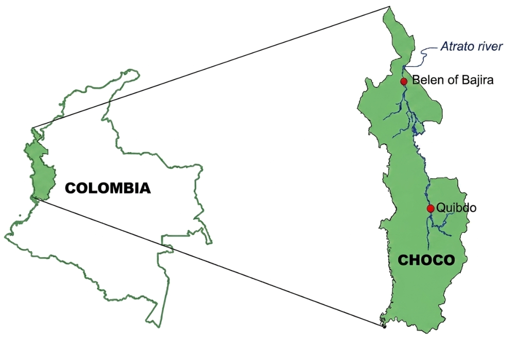Figure 1 shows the location of the hydrological stations and the exact place where the data collection of the study is performed in satellite form in the department of Chocó, Colombia, Atrato River.

In

Table 1. Description of the hydrological station locations.

	Station 1 (E1)	Station 2 (E2)
Longitude	76°40′10.75″ W	76°39′44.13″ W
Latitude	5°45′53.38″ N	5°41′52.77″ N
Altitude	20.579 MASL	20.83 MASL
City	Belén de Bajirá	Quibdó

, the geographical positions of the hydrological stations are shown.

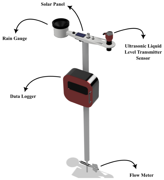
Figure 2 shows the prototype station considered for the case study of this article, which consist of an ultrasonic level sensor, a water flow sensor and a precipitation sensor.

Numerous strategically positioned measurement stations along the river enable tracking of variable dynamics in various locations. This inherent coupling among measurement variables facilitates the definition of a multivariate coupled model, allowing a comprehensive understanding of hydrological processes and interactions throughout the river system.

In addition, in

Table 2. Information of the used data sets.

Type	Organization	Available Data	Dataset
Station 1 (S1)	IDEAM	2021–2023	Flow, Level, Precipitation.
Station 2 (S2)	IDEAM	2021–2023	Flow, Level, Precipitation.

the information period of the data sets used and the specified hydrological variables of the system can be observed.

The water flow and precipitation in the Atrato River from the hydrological data of the two stations are used as input data, and the water level of the two hydrological stations is used as a prediction for model training. Thus, the system has a first-order structure with a training model structure of 4 inputs and 2 outputs.

A short-term LSTM network is a type of RNN designed to capture patterns in data sequences over immediate time periods. Unlike traditional RNNs, LSTMs feature memory units capable of retaining information over longer spans, but in this context, they focus on predicting events or behaviors in the short term without engaging in plagiarism practices [22].

The weights that can be learned from the LSTM layer are input weights W (InputWeights), recurrent weights R (RecurrentWeights) and bias b (Bias). The matrices W, R and b are the combination of input weights, cycle weights and offsets for each component, respectively. This layer connects matrices according to the following Equation (1):

$$\begin{array}{c}\hfill W=\left[\begin{array}{c}{W}_i\\ W_f\\ W_g\\ W_0\end{array}\right],R=\left[\begin{array}{c}{R}_i\\ R_f\\ R_g\\ R_0\end{array}\right],b=\left[\begin{array}{c}{b}_i\\ b_f\\ b_g\\ b_o\end{array}\right]\end{array}$$

(1)

where i, f, g and o determine the entry gate, forgetting gate, cell candidate and exit gate, respectively.

The cell state at time unit t is given by (2)

$$\begin{array}{c}\hfill C_t=f_t\odot C_{t-1}+i_t\odot g_t,\end{array}$$

(2)

where ⊙ determines the Hadamard product (element-level vector multiplication).

The hidden state at time unit t is given by (3)

$$\begin{array}{c}\hfill h_t=o_t\odot {\sigma }_c+C_t,\end{array}$$

(3)

where ${\sigma }_c$ determines the state activation function. By default, the lstmLayer function uses the hyperbolic tangent function (tanh) to calculate the state activation function.

The equations of the components in time unit t are described below. In (4), we describe the gateway equation entrance door, in (5) oblivion door, in (6) cell candidate and in (7) open door.

$$\begin{array}{c}\hfill i_t={\sigma }_g(W_i{u}_t+R_i{h}_{t-1}+b_i)\end{array}$$

(4)

$$\begin{array}{c}\hfill f_t={\sigma }_g(W_f{u}_t+R_f{h}_{t-1}+b_f)\end{array}$$

(5)

$$\begin{array}{c}\hfill g_t={\sigma }_c(W_g{u}_t+R_g{h}_{t-1}+b_g)\end{array}$$

(6)

$$\begin{array}{c}\hfill o_t={\sigma }_g(W_o{u}_t+R_o{h}_{t-1}+b_o)\end{array}$$

(7)

2.1. EnKF Forecasting

The state estimation ${\mathit{x}}_k$ can be obtained by applying the EnKF in two stages [23,24,25]. First, the forecast stage, where an ensemble of q forecasted state estimates is computed

$$\begin{array}{c}\hfill {\mathit{x}}_k^{f_i}=\mathit{F}({\overline{\mathit{x}}}_k^a,{\mathit{u}}_k)+{\mathit{\omega }}_k^i\end{array}$$

(8)

being $i=1,\dots ,q$, ${\mathit{\omega }}_k^i\in {\mathbb{R}}^{n\times 1}$ is a zero mean random variable with normal distribution an covariance ${\Omega }_k\in {\mathbb{R}}^{n\times n}$. The sample error covariance matrix computed from ${\mathit{\omega }}_k^i$ converges to ${\Omega }_k$ as $q\to \infty$. The forecasted measurement is given by

$$\begin{array}{c}\hfill {\mathit{y}}_k^{f_i}=f^{\ast }\left({\mathit{x}}_k^{f_i}\right)\end{array}$$

(9)

where $f_i$ denotes the i-th forecast ensemble member. Then, the ensemble mean for states ${\overline{\mathit{x}}}_k^f\in {\mathbb{R}}^{n\times 1}$ is defined by

$$\begin{array}{c}\hfill {\overline{\mathit{x}}}_k^f={\displaystyle \frac{1}{q}}{\displaystyle \sum _{i=1}^q}{\mathit{x}}_k^{f_i}\end{array}$$

(10)

and the ensemble mean for measurements ${\overline{\mathit{y}}}_k^f$ is defined by

$$\begin{array}{c}\hfill {\overline{\mathit{y}}}_k^f={\displaystyle \frac{1}{q}}{\displaystyle \sum _{i=1}^q}{\mathit{y}}_k^{f_i}\end{array}$$

(11)

The ensemble error matrix around the ensemble mean is defined as

$$\begin{array}{c}\hfill E_k^f=\left[\begin{array}{ccc}{\mathit{x}}_k^{f_1}-{\overline{\mathit{x}}}_k^f& \cdots & {\mathit{x}}_k^{f_q}-{\overline{\mathit{x}}}_k^f\end{array}\right]\end{array}$$

(12)

being $E_k^f\in {\mathbb{R}}^{n\times q}$, and the ensemble output error

$$\begin{array}{c}\hfill E_{y_k}^f=\left[\begin{array}{ccc}{\mathit{y}}_k^{f_1}-{\overline{\mathit{y}}}_k^f& \cdots & {\mathit{y}}_k^{f_q}-{\overline{\mathit{y}}}_k^f\end{array}\right]\end{array}$$

(13)

being $E_{y_k}^f\in {\mathbb{R}}^{d\times q}$, and where the forecast covariances are approximated as

$$\begin{array}{cc}\hfill P_k^f& ={\displaystyle \frac{1}{q-1}}{E}_k^f{\left(E_k^f\right)}^{\top }\hfill \\ \hfill P_{x{y}_k}^f& ={\displaystyle \frac{1}{q-1}}{E}_k^f{\left(E_{y_k}^f\right)}^{\top }\hfill \\ \hfill P_{y{y}_k}^f& ={\displaystyle \frac{1}{q-1}}{E}_{y_k}^f{\left(E_{y_k}^f\right)}^{\top }\hfill \end{array}$$

being $P_k^f\in {\mathbb{R}}^{n\times n}$, $P_{x{y}_k}^f\in {\mathbb{R}}^{n\times d}$ and $P_{y{y}_k}^f\in {\mathbb{R}}^{d\times d}$.

The second stage is the analysis stage, where an ensemble of perturbed observations ${\mathit{y}}_k^i$ is obtained as follows

$$\begin{array}{c}\hfill {\mathit{y}}_k^i={\mathit{y}}_k+{\mathit{\upsilon }}_k^i\end{array}$$

(14)

where ${\mathit{\upsilon }}_k^i\in {\mathbb{R}}^{d\times 1}$ is a zero mean random variable with normal distribution an covariance ${{\rm Y}}_k\in {\mathbb{R}}^{d\times d}$. The sample error covariance matrix computed from ${\mathit{\upsilon }}_k^i$ converges to ${{\rm Y}}_k$ as $q\to \infty$. Also, the EnKF gain matrix is approximated as

$$\begin{array}{c}\hfill K_k=P_{x{y}_k}^f{\left(P_{y{y}_k}^f\right)}^{-1}\end{array}$$

(15)

where it is worth noting that ${\left(P_{y{y}_k}^f\right)}^{-1}$ is an inverse of $d\times d$, being $d<<n$.

Therefore, an ensemble of data assimilation cycles is obtained as follows:

$$\begin{array}{c}\hfill {\mathit{x}}_k^{a_i}={\mathit{x}}_k^{f_i}+K_k\left({\mathit{y}}_k^i-f^{\ast }\left({\mathit{x}}_k^{f_i}\right)\right)\end{array}$$

(16)

where $a_i$ denotes the i-th analysis ensemble member. And finally, the ensemble mean of the analysis stage is computed as

$$\begin{array}{c}\hfill {\overline{\mathit{x}}}_k^a={\displaystyle \frac{1}{q}}{\displaystyle \sum _{i=1}^q}{\mathit{x}}_k^{a_i}\end{array}$$

(17)

where ${\overline{\mathit{x}}}_k^a$ is the estimated activity at sample k.

In order to validate the proposed approach, a comparative analysis of the LSTM model coupled and decoupled with a nonlinear recursive EnKF is developed. This evaluation is conducted using a state space model of the LSTM short-term recurrent neural network, aiming to validate the prediction capabilities of the nonlinear model for a system of fourth order. The dataset comprises data from two hydrological stations featuring four inputs and two outputs, and it is trained by using online training. We introduce four noise perturbations as variance parameters to assess the model’s robustness in level prediction. Visual comparisons between real and estimated signals for each noise parameter are presented for the LSTM model with the EnKF filter and the LSTM model without it. Additionally, a quantitative evaluation based on machine learning regression metrics is performed.

For a better description in

Table 3. Parameters of the LSTM model, LSTM-EnKF.

Non-Linear Models	# Input Nodes	# Hidden Nodes	# Output Nodes	Learning Rate	Epochs
ENKF	4	80	2	–	20
LSTM	4	40	2	0.02	20

presents the parameters used for the recurrent LSTM neural network and the EnKF algorithm, including the number of input, hidden, and output nodes, as well as the learning rate and number of training epochs.

Table 3 summarizes the configuration and training parameters of the proposed LSTM–EnKF model. The LSTM uses a sequence length of two time steps, corresponding to the previous 24 h of observations. The network comprises four input nodes, one hidden layer with 40 nodes, and two output nodes. It was trained for 20 epochs using the Adam optimizer with a learning rate of 0.02. The EnKF uses an ensemble size of $q=80$.

2.2. Hydrological Variables

Using the hydrological records from the two stations described previously, the forecasting problem is formulated as a nonlinear multivariate dynamic system. This formulation accounts for the temporal dependencies and cross-variable relationships among water level, flow, and precipitation. The input and output variables considered in the forecasting model are defined in Equation (18).

$$\begin{array}{c}\hfill {\mathit{y}}_k=\left[\begin{array}{c}{y}_{L_1}\left[k\right]\\ y_{L_2}\left[k\right]\end{array}\right],{\mathit{u}}_k=\left[\begin{array}{c}{u}_{F_1}\left[k\right]\\ u_{P{T}_1}\left[k\right]\\ u_{F_2}\left[k\right]\\ u_{P{T}_2}\left[k\right]\end{array}\right]\end{array}$$

(18)

where $y_{L_1}\left[k\right]$ and $y_{L_2}\left[k\right]$ correspond to the 2 outputs of the level variable of the two stations, $u_{F_1}\left[k\right]$, $u_{F_2}\left[k\right]$, $u_{P{T}_1}\left[k\right]$, and $u_{P{T}_2}\left[k\right]$ are the 4 inputs of the neural network system corresponding to the two stations of the multivariable system, i.e., the $u_{F_j}\left[k\right]$ represents the j-th 2 inputs of the flow variable of the two stations, and $u_{P{T}_j}\left[k\right]$ represents the j-th two more inputs of the rainfall variable of the two stations already mentioned, thus obtaining a multivariable system with 4 inputs and two outputs.

2.3. Regression Metrics for the Estimation of the Quadratic Error

In this study, the evaluation of predictive performance is essential to assess the quality of the model and to optimize its efficiency. Key indicators, such as Root Mean Square Error (RMSE), Mean Absolute Error (MAE) and Nash-Sutcliffe Model Efficiency (NSE) coefficient, are used to evaluate the prediction performance of the LSTM recurrent neural network model. The model includes noise in both input and output data for a configuration of 4 inputs and 2 outputs, designed for a fourth-order system. In addition, the LSTM model is combined with a nonlinear Ensemble Kalman filter (EnKF) to improve the estimation of the LSTM model by four noise variance parameters $(0.001,0.05,0.1,0.2)$.

$$\begin{array}{c}\hfill \begin{array}{c}\hfill RMSE=\sqrt{{\displaystyle \frac{1}{n}}{\Sigma }_{i=1}^n{(y_{0_i}-y_i)}^2}\end{array}\end{array}$$

(19)

$$\begin{array}{c}\hfill MAE={\displaystyle \frac{1}{n}}{\Sigma }_{i=1}^n[y_{0_i}-y_i]\end{array}$$

(20)

$$\begin{array}{c}\hfill \begin{array}{c}\hfill NSE=1-{\displaystyle \frac{{\Sigma }_{i=1}^n{(y_{0_i}-y_i)}^2}{{\Sigma }_{i=1}^n{(y_{0_i}-\overline{y_0})}^2}}\end{array}\end{array}$$

(21)

3. Results

Estimation Results

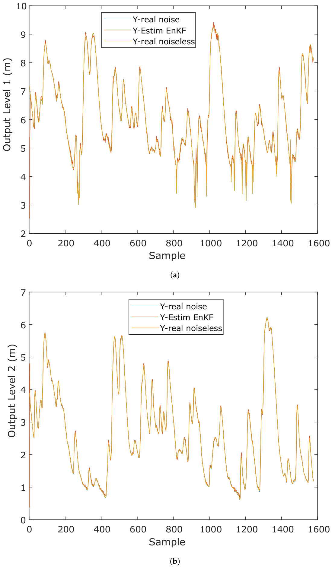
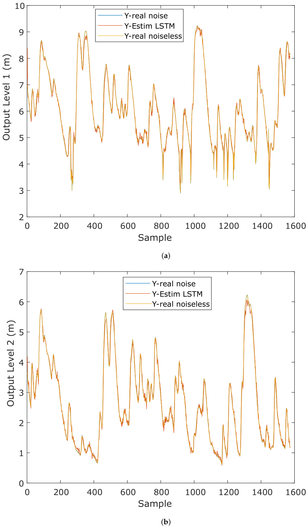
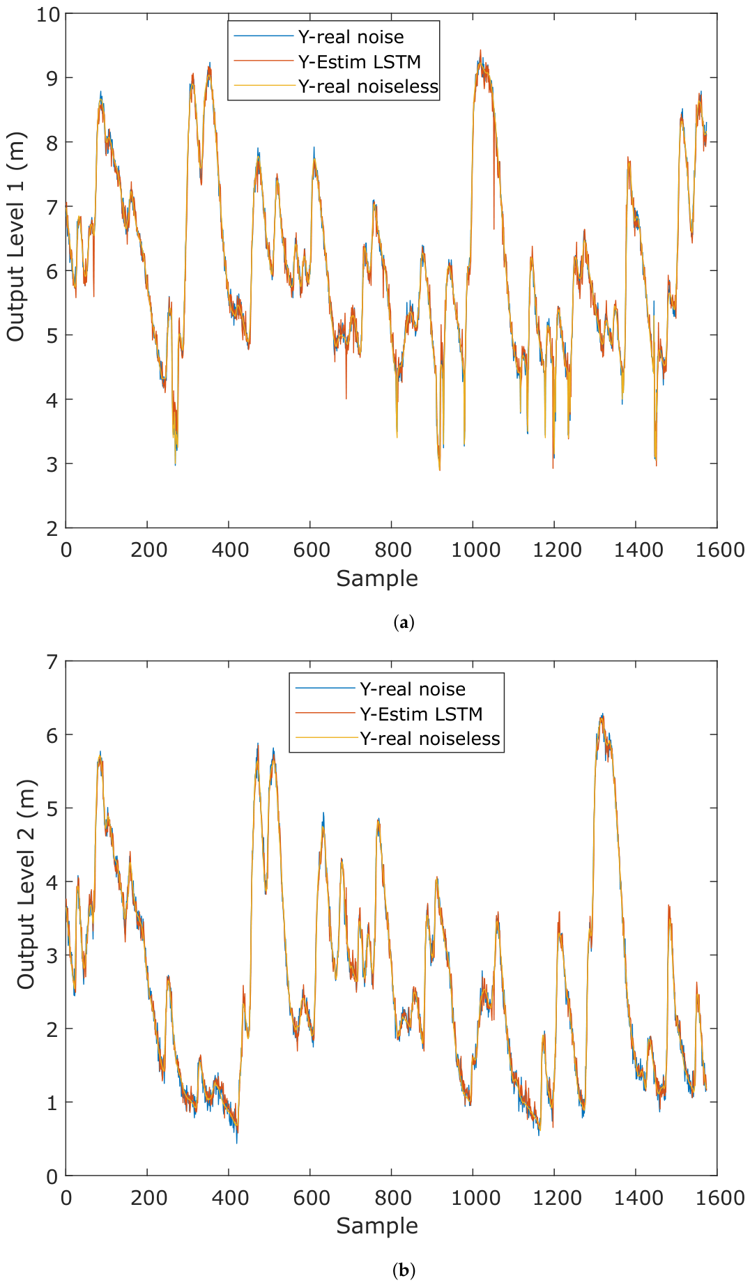
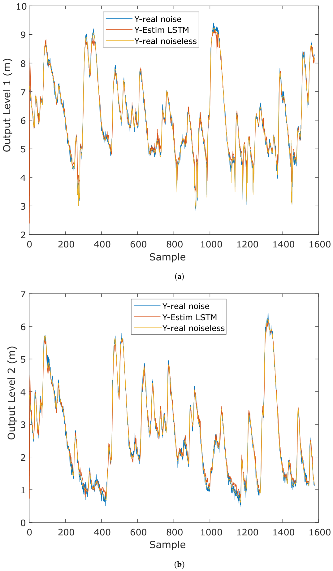
In this subsection are presented the forecasting results of the two methods considered: the multivariate LSTM approach coupled to an EnKF filter and the multivariate LSTM, where we obtain the responses of the real signal with noise in the images described as Y-real noise, the signal estimated with the LSTM-EnKF model, where it is described as Y-Estim EnKF, and the signal without noise.

Figure 3 and Figure 4 present the estimation results of the LSTM method coupled with the multivariate nonlinear recursive EnKF filter for two water level outputs. It uses 40 nodes in the LSTM hidden layer with white noise variance parameters of 0.01, 0.1, and 0.2, according to the results of the referenced tables. Figure 3 and Figure 4 the subfigures (a) and (b) show the estimation of the first and second water level outputs of hydrological stations, respectively. It is worth noting that Figure 3 and Figure 4 shows a comparison by using a fourth-order system of the measured real signal with noise, the estimated signal, and the real signal without noise.

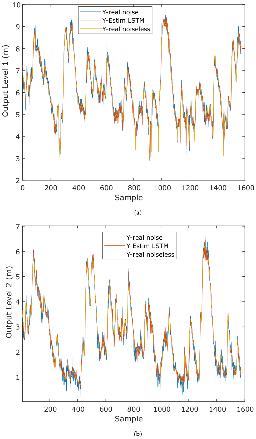
In Figure 5, Figure 6 and Figure 7 are shown the results of the estimation carried out using a multivariate LSTM neural network model, excluding the recursive nonlinear EnKF filter, for two water level outputs. The model comprises 40 nodes in the hidden layer and utilizes noise variance parameters set at 0.01, 0.1, and 0.2. In Figure 5, Figure 6 and Figure 7 the subfigures (a) and (b) are shown the estimations of the first and second water level outputs from hydrological station, respectively, considering a fourth-order system. The comparison includes the real signal with noise, the estimated signal, and the real signal without noise.

In addition,

Table 4. Root mean square estimation (RMSE) with Gaussian noise for LSTM neural network coupled with EnKF and without EnKF.

LSTM coupled with EnKF
Variance parameter	RMSE Output 1 (m)	RMSE Output 2 (m)	Total (m)
0.001	0.0533	0.0476	0.1009
0.05	0.0654	0.0533	0.1187
0.1	0.0823	0.0615	0.1438
0.2	0.1028	0.0901	0.1929
LSTM without EnKF
0.001	0.0970	0.0770	0.1740
0.05	0.0988	0.0871	0.1859
0.1	0.1124	0.0923	0.2047
0.2	0.1233	0.1123	0.2356

shows the RMSE estimates of the LSTM model without the EnKF filter and with the EnKF filter for the two outputs corresponding to the level of the hydrological variables for the two stations already described. It is worth mentioning that the EnKF implements the Bayesian Monte Carlo update problem: it updates the probability density function of the modeled system state.

In Table 4, a metric regression analysis of the data for the root mean square error (RMSE) estimates of an LSTM neural network with noise coupled to an EnKF and with decoupled noise without an EnKF is shown.

From Table 4, it is observed that the total estimation error of the Feedforward LSTM neural network is greater than the estimation error of the LSTM neural network coupled to the nonlinear recursive filter EnKF. It can be observed that the estimation of the two-station hydrological model used in this research presents an estimation of the model outputs. This can be observed in the calculated estimation error, which is quite low and well below 1. Also, the total estimation error of the recurrent neural network is observed to be larger than that of the LSTM neural network decoupled to the EnKF nonlinear recursive filter. It can be observed that the estimation of the two-station hydrological model used in this research presents an estimation. However, it can be observed that it does not have an optimal response as the LSTM neural network coupled to the EnKF.

A metric regression data analysis is shown for the Nash-Sutcliffe model efficiency coefficient (NSE) and Mean Absolute Error (MAE) for the LSTM neural network with noise coupled and decoupled to the EnKF filter.

A highlight of the results obtained in this study is the analysis of the Nash-Sutcliffe efficiency coefficient (NSE), a key indicator for assessing the quality of the predictions. A value of NSE close to 1 suggests that the predictions are optimal and that the model adequately describes the variability of the observed data. In the study, the performance of the LSTM model coupled and decoupled to the nonlinear recursive EnKF filter is analyzed by observing the impact of noise in the variance parameter on the NSE coefficient.

For the LSTM model without the EnKF filter, the NSE coefficient tends to move away from 1 as the noise in the variance parameter increases, indicating that the estimation quality decreases.

Table 5. Nash-Sutcliffe model efficiency coefficient (NSE) and Mean Absolute Error (MAE) with Gaussian noise for the LSTM neural network coupled with EnKF and decoupled without EnKF.

LSTM coupled with EnKF
Variance parameter	NSE Output 1 (m)	NSE Output 2 (m)	MAE Output 1	MAE Output 2
0.001	0.9916	0.9955	0.1042	0.1010
0.05	0.9917	0.9992	0.1190	0.1070
0.1	0.9866	0.9910	0.1233	0.1180
0.2	0.9760	0.9799	0.1322	0.1244
LSTM without EnKF
0.001	0.9683	0.9776	0.2380	0.2300
0.05	0.9432	0.9562	0.2475	0.2412
0.1	0.9301	0.9427	0.2667	0.2511
0.2	0.9200	0.9325	0.2863	0.2612

shows that for a noise in the variance parameter of 0.2, the NSE value is 0.9325 for output 2 of the LSTM model, suggesting that the prediction accuracy is lower with additional noise.

In contrast, for the LSTM model coupled to the EnKF filter, the NSE coefficient remains close to 1, even with noise in the variance parameter. In the same Table, for a variance noise of 0.2, the NSE value is 0.9799, indicating that the combination of LSTM and EnKF provides more reliable predictions. These results demonstrate the effectiveness of the EnKF filter in improving the stability and accuracy of LSTM model predictions, especially in noisy environments.

Another outstanding result is the mean absolute error (MAE), which shows that the LSTM recurrent neural network coupled to the EnKF filter shows an estimation error percentage of $10\%$ compared to the LSTM neural network without the EnKF filter, which shows an error percentage of approximately $20\%$ according to the MAE data obtained, this means that the EnKF filter coupled to the LSTM shows a decrease of $10\%$ of the percentage of error.

The LSTM (Long Short-Term Memory) model is an efficient recurrent neural network for handling long-term dependencies, which makes it suitable for river water level prediction. Configured with four inputs (precipitation, flow, upstream water level, and two outputs (water levels at two stations on the Atrato River), the LSTM offers some robustness to noise. However, its accuracy may decrease when faced with significant external disturbances.

The LSTM-ENKF model combines LSTM with the Ensemble Kalman Filter (ENKF), improving prediction capability and robustness to noise. ENKF adjusts LSTM predictions using new observations, which mitigates the impact of noise and results in more accurate estimates. This approach, although more accurate, involves greater complexity and demand for computational resources and processing time. In addition, the LSTM-ENKF is ideal when high accuracy is needed and sufficient resources are available due to its superior performance in the face of noise. However, in resource-constrained situations or where a simpler solution is required, pure LSTM may be sufficient, albeit with a possible reduction in accuracy under noisy conditions. The choice between the two models will depend on specific project objectives and operational constraints.

4. Discussion

The results show that coupling the LSTM network with the EnKF improves two-day-ahead water-level forecasting under all evaluated Gaussian white-noise conditions. The LSTM–EnKF achieved total RMSE values ranging from 0.1009 to 0.1929 m, compared with 0.1740 to 0.2356 m for the standalone LSTM, corresponding to reductions of approximately 18.1–42%. The hybrid model also produced higher NSE values (0.9760–0.9992) and reduced the MAE by approximately 51.9–56.2% across both outputs. These results indicate that assimilating observations through the EnKF reduces the forecasting errors generated by the standalone LSTM.

The improvement can be explained by the complementary functions of the two components. The LSTM learns nonlinear temporal dependencies and cross-variable relationships among water level, flow, and precipitation, whereas the EnKF updates the predicted states as observations become available. This sequential correction limits the propagation of errors caused by measurement disturbances. However, the RMSE reduction decreased from approximately $42\%$ at a noise variance of $0.001$ to $18.1\%$ at a variance of $0.20$. Thus, although the EnKF mitigates the effect of observational uncertainty, it does not completely eliminate the influence of increasingly noisy observations.

These findings are consistent with previous multivariate LSTM studies that demonstrated the ability of recurrent architectures to represent temporal and cross-station hydrological relationships [2,3]. The present study extends this line of research by incorporating sequential data assimilation and evaluating the coupled model under controlled noise conditions. It also builds on the previous NARX–EnKF framework [20] by replacing the predefined lag structure of NARX with the internal memory mechanism of the LSTM. Nevertheless, direct numerical comparisons should be interpreted cautiously because the datasets, prediction horizons, model configurations, and experimental conditions used in these studies may differ.

The two-day prediction horizon may provide useful information for flood preparedness and water-resources management along the Atrato River. However, the present findings represent an experimental evaluation rather than the validation of a complete operational early-warning system. Practical deployment would require real-time data transmission, automated data-quality control, operational warning thresholds, communication protocols, and validation during extreme hydrological events.

Methodological Uncertainties and Main Sources of Error

The results are subject to several sources of uncertainty. The hydrological records may contain measurement errors, missing observations, outliers, or inconsistencies associated with sensor operation, calibration, and data transmission. These errors can affect both the LSTM input sequences and the observations assimilated by the EnKF, thereby influencing the estimated states and the resulting forecasts.

The additive Gaussian white noise used in the experiments provides a controlled representation of measurement uncertainty and enables the models to be compared under reproducible disturbance levels. However, this assumption may not fully represent errors observed in operational hydrological monitoring systems. Real disturbances may be biased, temporally correlated, heteroscedastic, nonstationary, or associated with sensor malfunction and communication failures. Therefore, the reported robustness should be interpreted in relation to the specific noise assumptions evaluated in this study.

Model performance is also influenced by the LSTM architecture, hyperparameter configuration, training procedure, and random initialization. Variations in sequence length, number of hidden units, learning rate, number of epochs, and training-data composition may produce different forecasting results. Similarly, the EnKF is sensitive to the ensemble size, initial ensemble distribution, and specification of the process- and observation-error covariance matrices. Inadequate parameter or covariance selection may underestimate forecast uncertainty, reduce the effectiveness of state updates, or allow errors to propagate across the two-day forecasting horizon.

Finally, the analysis is limited to 789 days of observations from the Atrato River. This observational period may not fully represent interannual variability, seasonal transitions, or rare extreme-flood events. Consequently, the generalizability of the framework to other river basins, climatic periods, monitoring configurations, and hydrological conditions remains to be established. Further validation should therefore consider longer records, independent basins, additional monitoring locations, extreme-event data, and more realistic disturbance scenarios.

5. Conclusions

This study developed and evaluated a hybrid LSTM–EnKF framework for two-day-ahead multivariate water-level forecasting along the Atrato River. Combining the temporal-learning capability of the LSTM with the observation-assimilation mechanism of the EnKF improved forecasting performance relative to the standalone LSTM under all four Gaussian white-noise variance levels evaluated.

The LSTM–EnKF achieved total RMSE values ranging from 0.1009 to 0.1929 m, representing reductions of approximately 18.1–42% relative to the standalone LSTM. It also produced NSE values ranging from 0.9760 to 0.9992 and reduced the MAE by approximately 51.9–56.2% across both outputs. These results support the research hypothesis that sequential EnKF assimilation can reduce forecasting errors and maintain higher model efficiency under noisy observational conditions.

The principal methodological contribution is the integration of an LSTM network, which represents nonlinear temporal and cross-variable relationships, with an EnKF that recursively updates the estimated states using available observations. In this respect, the framework extends the previous NARX–EnKF formulation by replacing the predefined lag structure of NARX with the memory-based sequential representation provided by the LSTM.

Although the framework provides promising support for flood-risk management and early-warning applications, the conclusions are limited to the observational period, noise assumptions, hydrological setting, and model configuration evaluated in this study. Future research should validate the approach using longer records, independent river basins, additional monitoring locations, temporally correlated and non-Gaussian disturbances, and a broader representation of extreme-flood events. Further studies should also examine ensemble-size sensitivity, covariance specification, hyperparameter uncertainty, computational requirements, and operational implementation using real-time hydrological observations.