


Abstract
Cut-cell and ghost-cell finite-volume methods require an accurate boundary distance field, available in closed form only for simple shapes and otherwise obtained through costly nearest-neighbor search. Prior work embeds learned distance fields as an auxiliary component inside a larger neural architecture; this study instead tests the numerical consequences of substituting the distance function alone within an otherwise unmodified classical discretization. We propose a compact trained neural network as a drop-in surrogate for this field, evaluated against exact and classical alternatives, including a KD-tree baseline, on four problems of increasing difficulty ending with a three-dimensional mechanical flange. A truncation analysis bounds the surrogate’s intercept error and identifies the training accuracy needed to preserve the scheme’s formal order. The surrogate matches second-order accuracy in every example, with fitted orders of 2.0 to 2.1 in two dimensions and, in three dimensions, a wider but still order-consistent 1.9 to 2.5, the extra width traced to identified, shared mesh- and timestep-resolution effects rather than to the surrogate itself. Query cost overtakes the KD-tree beyond roughly one hundred thousand points, with speedups up to 26.1 times, and gradient fields are substantially smoother than nearest-point construction throughout, tracking geometric severity in two dimensions and feature scale in three.
1. Introduction
Many problems in computational physics and engineering require solving partial differential equations on domains whose boundaries do not align with a simple structured grid. Embedded-boundary approaches address this mismatch by keeping the underlying computational grid Cartesian and modifying the discretization near the interface, avoiding the cost and fragility of repeated body-fitted remeshing. The earliest and most influential example is the immersed boundary method, introduced by Peskin [1,2] to simulate blood flow around heart valves and later formalized and reviewed at length [3,4]. Sharper and more local treatments of the interface followed by embedded-boundary finite-volume discretizations of the Poisson equation were presented in [5], the ghost-fluid method for multimaterial and multiphase flows was introduced by [6], and the second-order-accurate symmetric cut-cell and ghost-cell schemes for irregular domains on which the present work builds directly, proposed mainly by [7]. A closely related family of methods represents the interface itself as the zero level set of an auxiliary function evolved on the background grid [8,9,10,11], which again requires an accurate distance or implicit field defined throughout a neighborhood of the boundary.
Every method in this family shares a common numerical requirement, which is an accurate signed or unsigned distance field indicating how far a given point lies from the boundary and in which direction the boundary lies. When the domain is described by a closed-form expression, this distance field is available exactly, and the resulting solver achieves whatever accuracy the underlying stencil affords. However, real engineering and scientific geometry is rarely available in closed form. A digitized airfoil cross-section, a triangulated CAD part, or a laser-scanned physical object is described only by a discrete set of points or a polygon mesh, and the distance to such a set must be constructed algorithmically rather than evaluated analytically. The naive approach, brute-force search over every boundary point, scales linearly with the number of points and quickly dominates solver cost as geometric resolution increases. Spatial indexing structures, most notably the KD-tree [12,13], substantially reduce this cost through a one-time build followed by logarithmic-time queries, and this is the classical baseline a fair comparison must use rather than brute force alone. For raw scan data specifically, computer graphics has developed dedicated pipelines for turning unorganized point clouds into usable surface and distance representations, including volumetric range-image fusion into a cumulative signed distance field [14] and Poisson-equation-based surface reconstruction from oriented points [15]. All of these discrete constructions, spatial index or reconstructed mesh alike, inherit a property of the underlying point set that is often overlooked in this context, since the nearest-point direction is piecewise constant and changes discontinuously wherever the identity of the closest boundary point switches. The resulting distance field is continuous, but its gradient, which is defined as the outward normal direction used throughout an embedded-boundary stencil, is not.
This paper investigates the use of a compact trained neural network as a smooth, fixed-cost surrogate for the boundary distance function within an otherwise standard cut-cell finite-volume solver. The surrogate is evaluated against exact and classical discrete distance representations using three complementary criteria relevant to numerical discretization rather than shape reconstruction or operator learning. First, verification establishes whether replacing the exact or point-cloud-based distance function with the neural surrogate preserves the formal order of accuracy of the underlying finite-volume scheme. Second, computational cost scaling quantifies the efficiency of the surrogate relative to an optimized KD-tree nearest-neighbor search, the strongest classical baseline available for this task, identifying the problem sizes at which its constant per-query evaluation becomes computationally advantageous; because a trained network and a spatial search are different computational primitives—a fixed-cost forward pass set against a repeated, logarithmic-cost query—rather than two implementations of the same operation; the resulting crossover points are best read as a conservative bound specific to this search-based comparison, with the larger gains a trained surrogate typically offers realized instead against costlier direct calculations it might replace, such as a full field solve. Third, gradient smoothness assesses whether the differentiable neural representation provides a smoother normal-direction field than conventional nearest-point constructions and examines how this benefit varies with local boundary geometry.
These performance criteria are examined using four benchmark problems selected to represent progressively increasing geometric complexity and practical relevance. The first benchmark is a smooth five-lobed closed curve with an analytical signed-distance function, providing a fully controlled environment for verification. The second is a multiply connected domain containing two circular holes and a narrow reentrant slit, enabling a systematic assessment of gradient smoothness under varying levels of local geometric complexity. The third benchmark employs the digitized Selig S1223 airfoil cross-section, originally reported in a low-speed wind-tunnel study [16] and obtained directly from the UIUC Airfoil Coordinates Database [17]. In this case, no analytical geometry is available, and all reference distances are computed directly from the boundary point cloud, thereby evaluating the surrogate under realistic engineering conditions. The final benchmark is a three-dimensional mechanical mounting flange consisting of a circular plate with a central bore and six bolt holes, representing a practical engineering component. This example extends the investigation to a genuine three-dimensional cut-cell finite-volume problem, allowing verification, computational cost scaling, and gradient smoothness to be assessed beyond two dimensions while examining the robustness of the proposed surrogate in the presence of complex internal geometric features.
Throughout the study, all results are reported comprehensively, including scenarios in which the proposed neural surrogate does not outperform established methods. In particular, the KD-tree nearest-neighbor search remains computationally more efficient for small boundary point sets, and the corresponding crossover points are identified quantitatively rather than omitted. When the neural surrogate provides improved gradient smoothness, the magnitude of this benefit is shown to increase with local geometric complexity in the two-dimensional benchmarks. The three-dimensional study reveals a more nuanced behavior, where the improvement correlates more strongly with geometric feature scale than with concavity, thereby highlighting dimensional differences in the underlying mechanisms. Furthermore, the reported smoothness characteristics are demonstrated to be insensitive to the selected standoff distance, while the consistency of the neural surrogate is established through repeated training using multiple random initialization seeds rather than a single realization.
The remainder of the paper is organized as follows. Section 2 reviews the relevant literature and identifies the research gap addressed in this work. Section 3 presents the cut-cell finite-volume formulation, the five boundary closure schemes together with their truncation-error analysis, the origin of gradient non-smoothness in discrete nearest-point representations, and the proposed neural distance surrogate, including an analytical bound on the resulting intercept error. Section 4 describes the benchmark problems and evaluation methodology, Section 5 presents and discusses the numerical results, and Section 6 summarizes the main findings and conclusions.
2. Related Work
Neural representations of signed distance functions (SDFs) have become a well-established paradigm in computer graphics and geometric modeling. DeepSDF presented in [18] demonstrated that compact multilayer perceptrons can represent complex geometries through the zero level set of a learned continuous function, while Occupancy Networks introduced a closely related implicit occupancy representation for three-dimensional shape reconstruction in [19]. Subsequent developments in coordinate-based neural fields, including neural radiance fields (NeRFs), further established the effectiveness of continuous neural representations for geometric modeling and highlighted the spectral bias of standard coordinate networks toward low-frequency functions, motivating Fourier feature encodings and periodic activation functions to improve geometric fidelity [20,21,22,23]. Despite their success, these approaches have been developed primarily for geometry representation, compression, reconstruction, and rendering rather than as numerical components within classical PDE discretizations.
The integration of neural networks into numerical PDE solution methods has a much longer history, beginning with early feedforward-network approximations of ODE and PDE solutions [24,25] and evolving into physics-informed neural networks (PINNs), which incorporate the governing equations directly into the training objective [26]. Recent research has increasingly incorporated signed distance functions into this framework. Sukumar and Srivastava in [27] employed approximate distance functions to enforce Dirichlet boundary conditions exactly within PINNs. PhyGeoNet introduced a geometry-aware physics-informed architecture based on coordinate transformations rather than learned distance fields [28], while Oldenburg et al. combined variational autoencoder shape embeddings with PINNs to construct geometry-aware surrogates for Navier–Stokes flow over complex domains in [29]. More recently, geometry-informed neural operators have incorporated signed-distance representations to learn solution operators across families of geometries [30]; DeepONet-based approaches in [31] have integrated signed-distance and derivative-based constraints to improve boundary accuracy, and latent shape encodings based on signed distance functions have enabled mesh-free surrogate models for irregular domains in [32].
Beyond the coordinate-based multilayer perceptrons discussed above, other function-approximation paradigms have recently emerged for learning a smooth field from scattered samples. Kolmogorov–Arnold Networks replace the fixed node activations of a standard perceptron with learnable edge functions [33], and have been extended to a wavelet-based variant, Wav-KAN [34]; separately, higher-order Haar wavelet discretizations have been developed and applied to boundary value problems in structural mechanics, achieving high accuracy at reduced computational cost relative to the classical, first-order Haar wavelet method [35].
Collectively, these studies demonstrate that learned distance representations provide an effective mechanism for incorporating geometric information into neural PDE solvers and operator-learning frameworks. However, the learned distance field is consistently treated as an auxiliary component of a larger neural architecture rather than as an independent replacement for the geometric information required by a conventional numerical solver. Consequently, the numerical implications of substituting the distance function alone within an otherwise unchanged finite-volume discretization have not been systematically investigated. In particular, previous studies have not examined whether such a substitution preserves the formal accuracy of the underlying discretization, how its computational cost compares with optimized classical spatial-search structures such as KD-trees, or whether the resulting continuous representation provides measurably smoother normal-direction fields than discrete nearest-point constructions. Addressing these three aspects constitutes the primary contribution of the present work.
3. Mathematical Formulation and Numerical Framework
This section establishes the mathematical and numerical foundations of the proposed framework. It begins by formulating the continuous problem (Section 3.1) and defining the properties of the signed distance function required by the solver (Section 3.2). The cut-cell finite-volume discretization is then presented, together with the five boundary closure treatments and their local truncation error analysis (Section 3.3 and Section 3.4). The discussion subsequently reviews classical discrete signed-distance constructions and analyzes the structural non-smoothness of their gradients (Section 3.5). The section concludes by introducing the neural surrogate, characterizing the error it induces in the boundary closure, and detailing the training procedure and reproducibility protocol (Section 3.6).
3.1. Continuous Problem
Let ( or 3) be an open, bounded domain with piecewise-smooth boundary , embedded in a rectangular computational box . We consider the linear advection–diffusion initial–boundary-value problem: find satisfying the governing equation
subject to the Dirichlet boundary condition
and the initial condition
with constant velocity in two dimensions, in three, and diffusivity throughout. Verification follows the method of manufactured solutions [36,37], and the source term is constructed so that a prescribed smooth field satisfies Equation (1) exactly, with the boundary and initial data of Equations (2) and (3) taken as the corresponding traces of that field (so that Equations (2) and (3) hold by construction rather than by cancellation). In two dimensions the manufactured field is
and substituting Equation (4) into Equation (1) gives, in closed form,
In three dimensions (Example 4), the manufactured field is the direct extension
with the corresponding source term
the diffusive coefficient changes from to because the Laplacian gains a third second-derivative term. In both cases, the Dirichlet and initial data are the traces and . Because , the discretization error is measurable pointwise and the convergence rates reported in Section 5 are accurate and free of reference-solution ambiguity.
3.2. The Signed Distance Function
The signed distance function of is defined as
The function is Lipschitz continuous with constant 1, satisfies the eikonal equation wherever it is differentiable, and in a tubular neighborhood of a boundary () is itself , with restricted to equal to the outward unit normal under the sign convention of Equation (8), which takes negative inside ; some computer-graphics implementations adopt the opposite convention, which simply reverses the sign of and hence of the normal, and every quantity used downstream in this work—the intercept , the closure formulas of Section 3.4, and the smoothness metric of Section 3.5—depends only on the zero level set and on , not on which sign is chosen. The interested reader is directed to [38] for a detailed review of level set methods. Two consequences drive everything that follows. First, the zero level set locates the boundary implicitly, so any sufficiently accurate approximation of near locates the boundary to the same accuracy. Second, the normal field a sharp embedded-boundary method uses is exactly evaluated near the interface, so the smoothness of an approximation to —not merely its accuracy—is inherited directly by the normal field the solver consumes.
3.3. Cut-Cell Finite-Volume Discretization
The box B is discretized by a uniform Cartesian grid of cell centers with spacing h ( centers in two dimensions; in three, with set by the box aspect ratio), and the active index set collects the multi-indices of the cell centers lying in ; only active cells carry unknowns. Away from the boundary, the diffusion operator is the standard five-point (two-dimensional) or seven-point (three-dimensional) Laplacian with truncation error , and the advective derivative is approximated by centered differences.
Time integration uses an implicit–explicit (IMEX) splitting presented in [39,40] where the stiff diffusive term is advanced by backward Euler, which is unconditionally stable, while the non-stiff advective term is advanced by the classical fourth-order Runge–Kutta scheme with boundary-adjacent stencil values supplied by ghost values interpolated from the Dirichlet data. Each step solves one sparse linear system
where is modified near as described in Section 3.4, with , , and the grid ranges of Section 4. The advective Courant number remains below on every grid of every example. On the two-dimensional grids, the temporal error of the splitting is far below the spatial error, so the measured convergence rates there isolate the spatial error and, more specifically, the boundary-treatment error. On the finest three-dimensional grids of Example 4 this margin narrows—the backward-Euler diffusion step is only first-order in time, and at the finest grid and are of comparable magnitude—a point returned to when interpreting that example’s convergence data (Example 4).
3.4. Boundary Closures
Let be an active cell center with a neighbor (grid direction ) lying outside , so that the link crosses . The boundary intercept fraction is the unique root
Assuming a single transversal intersection of each grid link with the immersed boundary, an assumption satisfied for all meshes considered once the geometry is adequately resolved, each boundary closure is constructed independently on a one-dimensional cut link. Consequently, the formulation is identical in two and three spatial dimensions, differing only in the number of coordinate directions associated with each control volume. Figure 1 illustrates the three fundamental closure families considered in this work: the naive boundary-aligned closure, the linear-intercept (Shortley–Weller) closure, and the quadratic ghost-cell closure. The five boundary treatments investigated in this paper are obtained from these families by varying the source of the boundary intercept or the interpolation order, as detailed below.
Figure 1.
The three families of boundary closures along one cut grid link. (a) Naive: the Dirichlet value g is imposed at the exterior cell center, displacing the boundary by ; this is the negative control. (b) Linear intercept: the boundary crossing at fraction of the link defines a ghost value by linear extrapolation, Equation (11). (c) Quadratic ghost cell: the second interior neighbor enters with the Lagrange weights of Equation (15).
- 1.
- Naive (). The Dirichlet value is imposed at the exterior cell center itself, i.e., the boundary is snapped to the grid. The interface is thereby displaced by an distance that does not vanish relative to the stencil, producing an relative error in the boundary condition placement; no convergence beyond order zero should be expected. This closure is retained purely as a negative control.
- 2.
- Exact-SDF (linear intercept). The classical Shortley–Weller-type dimension-by-dimension closure presented in [7,41] where a linear interpolant through and defines the ghost value at ,which, substituted into the standard second difference, yields the modified rowwith the interior neighbor opposite the cut. Taylor expansion about shows the local truncation error of Equation (12) is at cut cells, but since these form a codimension-one set, global second-order accuracy in the discrete norm is retained [7]; the convergence studies of Section 5 confirm this. Here is computed from the exact geometry (analytically or by bisection on the inside/outside predicate).
- 3.
- Neural-SDF. Identical to closure 2, except that is obtained from the trained surrogate by linear inversion of the predicted level set along the link,where the lower clip excludes the ill-conditioned limit (the standard remedy in ghost-cell methods, where vanishing makes the row coefficient unbounded [7]). Equation (13) is the only point at which the network enters the solver; everything downstream is unchanged classical numerics (illustrated schematically in Section 3.6 below). The error this substitution introduces is quantified in Proposition 1 below.
- 4.
- Cut-cell (conservative). Closure 2 combined with a finite-volume weighting of the temporal term by the cell volume fraction , estimated by subcell sampling of the inside/outside predicate, so that the update approximates rather than the pointwise derivative; this is the standard conservation-oriented cut-cell variant. Interested reader is referred to [5,42,43,44] for a detailed construction mechanism.
- 5.
- Ghost-cell quadratic. The quadratic extrapolation of Gibou et al. [7], in which the ghost value is the quadratic Lagrange interpolant through , , , evaluated at ,with weightssatisfying and, at , as required, giving an local truncation error at cut cells. Wherever the second interior neighbor is unavailable—e.g., in thin regions of the domain—the scheme falls back to Equation (11).
Each closure plays a distinct role in the study. The naive closure establishes that the test problems are genuinely sensitive to boundary accuracy; the exact-SDF closure establishes the attainable ceiling of the linear intercept family and the remaining three probe whether that ceiling is reached by, respectively, a learned , a conservative variant, and a formally higher-order completion. The accuracy cost of replacing by admits a sharp elementary bound.
Proposition 1 (Intercept error of the neural closure).
Let in a neighborhood of the cut link , and suppose the crossing is transversal in the sense that for all on the link and some (the interface is not tangent to the grid direction ). Suppose further . Then the intercept of Equation (13) (before clipping and neglecting the fixed regularization , which is negligible whenever ) satisfies
where denotes the supremum on the link of the second directional derivative of ϕ along , and consequently the boundary-placement error in the Dirichlet data obeys
Proof.
Write for , so . By the chain rule, , so the transversality hypothesis gives for every ; in particular is strictly monotonic on ; so is its unique root, and by the mean value theorem for some .
Let be the linear interpolant of the exact values , and let be its root. Standard linear-interpolation theory gives , so . By the mean value theorem applied between and , together with ,
Now let be the linear model built from the surrogate’s endpoint values, whose root (before clipping) is . For every ,
since and each term is bounded by . Because L is linear with , and has magnitude at most by Equation (19) while ,
Remark 1.
Equation (17) establishes the accuracy requirement that the neural surrogate must satisfy to preserve the second-order convergence of the corrected solver. Specifically, it is sufficient that the signed-distance approximation error obeys in the vicinity of the immersed boundary as the mesh is refined. In the present framework, the surrogate is retrained independently on each grid using cell-center samples from that grid. Consequently, the density of the near-boundary training data increases naturally with mesh refinement, allowing the attainable approximation error to decrease consistently with h. Whether this asymptotic scaling is achieved is verified numerically in Section 5.1. The observed global convergence rates of approximately –, together with their narrow confidence intervals, confirm that the required accuracy is attained across all resolutions considered. Under this condition, the induced intercept error in the neural boundary closure is , matching the truncation error already tolerated by the exact-SDF cut-cell discretization (Section 3.4). Consequently, the surrogate is required only to resolve the geometry at the accuracy dictated by the mesh, rather than to achieve uniform accuracy throughout the computational domain. The clip at in Equation (13) lies outside the scope of the bound in Equation (16), which is stated for the unclipped root of the linear model; it engages only when that root would otherwise fall below , which by the same bound requires itself to lie within of the clip boundary, since the neural and exact roots cannot differ by more than this amount. Such near-boundary links form a shrinking, codimension-one subset of the cut cells as —the same class already responsible for the local truncation error tolerated by the exact-SDF closure without affecting its global second-order rate—so the clip is expected, and observed (Section 5.1), to leave the global convergence rate unaffected.
3.5. Classical Discrete Distance Constructions and Their Gradient
When is known only through a finite sample , the computable object is the point-set distance
Two exact algorithms for Equation (21) serve as classical baselines. Brute-force search costs per query with no setup. The KD-tree [12,13], whose practical performance and modern variants continue to be benchmarked and revisited [45,46], costs to build once and expected time per query thereafter, and is the appropriate classical baseline for any comparison that accounts for the setup-versus-query overhead asymmetry. Both algorithms compute the same function , and has a structural property independent of the search algorithm. Let denote the Voronoi cells of P [47]. In the interior of each ,
a unit vector pointing along the line to the single nearest sample; itself is Lipschitz and continuous everywhere, but Equation (22) shows its gradient is piecewise constant in direction along any query path within one Voronoi cell and jumps discontinuously across every Voronoi face, where the identity of the nearest sample switches, exactly as seen in the direction arrows of Figure 2a, each pointing to a different sample once the query crosses a dotted bisector. At a point on the face between and at distance from two consecutive samples spaced s apart, the jump angle is , i.e., ; the resulting discontinuities are the step jumps in the nearest-point angle trace of Figure 2b, plotted against the smooth surrogate-gradient curve it oscillates about. Refining the sample (smaller s) shrinks each individual jump but proportionally multiplies their number, while querying closer to the boundary (smaller ) makes every jump larger.
Figure 2.
Structural non-smoothness of the discrete nearest-point normal. (a) The gradient of the point-set distance , Equation (22); arrows show its direction, which points toward whichever sample is currently nearest, so the direction is constant within each Voronoi cell (dotted lines mark the Voronoi cell boundaries) and jumps by across each face. (b) Direction angle along an offset query path, where the nearest-point field is a staircase and a smooth surrogate gradient follows the continuous normal. Where the underlying angle is monotone, the two have equal total variation; excess variation, Equation (29), appears where concave geometry makes the staircase non-monotone.
Remark 2.
The total-variation metric of Section 4.4 does not automatically favor a smooth field. If the direction angle of the true normal is monotone along the query path—as it is outside a convex boundary component at small offset—the nearest-point staircase and the smooth field accumulate the same total variation, and the ratio between them approaches one. Excess variation arises precisely where concave or reentrant geometry makes the nearest-sample identity oscillate between distinct boundary sub-arcs, each reversal contributing jumps that the smooth field does not make. The theory, therefore, predicts a smoothness ratio near unity on convex components and growing with local concavity—a prediction tested, and confirmed, by the per-component measurements of Section 5.3.
3.6. Neural Distance Surrogate
The surrogate is a fully connected multilayer perceptron ,
where , , and are the weight matrices of the first hidden layer, the second hidden layer, and the linear output layer; and are the corresponding bias vectors; is the scalar output bias and are the hidden-layer widths (30 or 40, per example, Table 1). Because every network in this study uses exactly two hidden layers, Equation (23) is written directly in terms of these three weight matrices, mapping raw coordinates to a scalar distance, as shown in Figure 3a. Such networks are dense in the continuous functions on compact sets [48,49,50], so the representation itself imposes no accuracy floor; the practical floor is set by optimization and by the well-documented spectral bias of coordinate networks toward low-frequency functions [21,22,23]. Deliberately, no Fourier feature encoding, periodic activation, or other specialized machinery is used, since part of the purpose of the study is to establish what an off-the-shelf regression network achieves in this role, in preference to architectures such as radial-basis-function networks or, more recently, Kolmogorov–Arnold Networks and their wavelet variant Wav-KAN [33,34], whose basis- or edge-function counts typically scale with the size of the training set; this would be an unwelcome property here, since the surrogate is retrained from scratch, on training sets spanning three orders of magnitude, at every grid level and in both two and three dimensions. A systematic comparison against such alternatives is left to future work (Section 6).
Figure 3.
The neural distance surrogate and its single point of entry into the solver. (a) Architecture for the two-dimensional examples: raw coordinates in, scalar distance out, Equation (23); no positional encoding. (b) Schematic level sets of a signed-distance field for the Example-1 geometry, colored by the value of (level-set contours), illustrating the construction the trained surrogate is meant to reproduce; on a cut grid link (interior center filled, exterior open), the two field values determine the intercept of Equation (13) (star), the only quantity the network supplies to the otherwise classical scheme. The star lies on the straight segment between the two nodes rather than on the curved boundary itself, illustrating the small intercept error quantified in Proposition 1.
Training minimizes the mean-squared error
over sample–target pairs . For the two-dimensional examples the network has two hidden layers of 30 units (Examples 1 and 3) or 40 units (Example 2, whose multiply-connected boundary requires more capacity), the width in each case set by a preliminary sweep over 15–60 units per layer at the finest grid, retaining the smallest width beyond which doubling it reduced the training-set signed-distance error by less than ten percent, a pragmatic capacity-selection procedure consistent with that adopted in other recent design-optimization studies using compact feedforward networks [51]. Training runs for 100 epochs by the Levenberg–Marquardt method [52,53,54], whose update solves
with J the Jacobian of the residual vector and the damping parameter adjusted adaptively at every step—decreased by a factor of ten after an epoch that reduces the loss, increased by the same factor, with the step recomputed, otherwise, from an initial up to a ceiling of beyond which training would be judged to have diverged, though no run in this study approaches that ceiling—the method of choice for small dense least-squares networks of this size. The training set is the set of cell centers of the current grid, with signed-distance targets computed exactly from a dense polyline representation of the boundary; consistent with standard practice for this training routine, the sample set is further partitioned at random into 70% training, 15% validation, and 15% test subsets, and training is halted early should the validation error fail to improve over six consecutive epochs, the only regularization applied beyond the network’s modest capacity, since the deterministic, noise-free geometric targets leave comparatively little for a validation split to guard against beyond monitoring convergence itself; at the finest grid of every example, the held-out validation error exceeds the training error by a factor of only –, with the test error tracking the validation error just as closely, confirming that this split finds no meaningful generalization gap to guard against. The network is retrained from scratch at every grid level (cf. Remark 1), so no network is ever reused across resolutions and training cost is charged at every level.
The three-dimensional example (Example 4) follows the same recipe, with two hidden layers of 40 units, again the width set by the capacity sweep described above and required here by the bore-and-bolt-hole geometry, grid-center training data, and signed-distance targets computed from a dense surface point cloud together with the domain’s exact containment predicate. The only change is the optimizer at the two finest grids, since Levenberg–Marquardt’s Jacobian-based update of Equation (25) scales with the product of training-set size and parameter count, and at these grids’ 69,360 and 134,064 training points it becomes the dominant cost, so those two networks are trained for 1000 epochs by scaled conjugate gradient [55], which avoids forming ; every coarser grid retains the 100-epoch Levenberg–Marquardt setup used in two dimensions.
Three reproducibility safeguards apply to every experiment. First, all training runs are seeded, with a distinct documented seed per grid level, making every reported number exactly regenerable. Second, because one random initialization yields one draw of the trained network, the finest-grid configuration of each PDE example is retrained five times from independent seeds and the spread of both the final solution error and the training time is reported as an explicit uncertainty; across every example this spread is two to three orders of magnitude smaller than the error itself, indicating that the trained result does not hinge on a favorable initialization—a conclusion reinforced wherever the network is queried away from its own training locations elsewhere in the study, whether by the smoothness and cost-scaling benchmarks of Section 4.4 and Section 4.3, which sample points off the training grid, or by the solver itself, whose boundary intercept of Equation (13) coincides with a training point only in the non-generic case , so that the second-order convergence of Section 5.1 is itself measured off the training set. This repeated-seed check is deliberately concentrated at the finest grid of each example, where the accuracy floor required by Remark 1 is tightest and any seed sensitivity would be most exposed; it establishes that the finest-grid result is not a favorable draw, but it does not by itself characterize how the seed-to-seed spread scales with h, since every coarser grid in the convergence study is trained from a single documented seed rather than repeated. Third, one-time costs are accounted symmetrically, with the network’s training time always reported alongside the KD-tree’s build time as the analogous setup investment, so the fixed-query-cost advantage claimed for the surrogate is never obtained by silently amortizing its training away.
4. Test Problems and Evaluation Protocol
4.1. Test Problems
The numerical assessment comprises four benchmark problems spanning a broad range of geometric complexity, from smooth analytical geometries to raw digitized data, and from two- to three-dimensional domains. The examples are arranged in increasing geometric and practical complexity, beginning with a smooth analytical benchmark that admits an exact reference solution and progressing toward realistic engineering geometries.
Example 1 (flower).
The boundary is the smooth closed curve , producing five shallow concave lobes. A dense polyline of 1500 vertices represents the boundary for the distance targets and all point-cloud baselines, while the analytical description provides the exact intercepts of Equation (10). The convergence study employs ten grids, .
Example 2 (multiply-connected domain).
The domain consists of a mildly irregular disk, , containing two circular holes and a narrow reentrant slit extending inward to , thereby introducing two sharp reentrant corners. This geometry combines smooth and non-smooth boundary components within a single controlled benchmark, enabling the component-wise assessment discussed in Remark 2. The grid sequence and PDE configuration are identical to those of Example 1, with exact intercepts computed by bisection on the analytical inside/outside predicate.
Example 3 (digitized airfoil).
The Selig S1223 airfoil cross-section [16], obtained directly from the UIUC Airfoil Coordinates Database [17], consists of 81 digitized points at unit chord. Since no analytical representation is available, the reference geometry is defined by a fine spline interpolant through the raw data, parameterized by cumulative arc length. Owing to the thin airfoil profile, the convergence study employs , with formal convergence measured only on sufficiently resolved grids (Section 4.2). The cut-cell and quadratic ghost-cell closures are omitted here because their extra machinery—respectively, subcell sampling of an inside/outside predicate for the volume fraction, and a reliable second interior neighbor near a thin, curved boundary—is a separate implementation burden from the one this study is built to isolate. The comparison this paper is designed around, exact geometry against the trained surrogate on an otherwise identical closure, is the linear-intercept pair (closures 2 and 3) and is present in every example, including this one; only the cut-cell and quadratic completions are narrowed to the examples with an available exact predicate, where they were already exercised in Examples 1 and 2. Only the naive, exact (point-cloud), and neural-SDF closures are compared.
Example 4 (mechanical mounting flange).
The final benchmark is a three-dimensional mechanical mounting flange consisting of a circular plate with a central bore and six equally spaced bolt holes (a three-dimensional rendering appears later in Section 5, Figure 13). Unlike Example 3, the geometry is defined analytically through constructive solid geometry, permitting an exact inside/outside predicate, exact boundary intercepts, and a manufactured-solution verification in three dimensions. As in Example 3, only the naive, exact, and neural-SDF closures are compared, so that the same three-way comparison is reported uniformly across all four benchmarks; extending the cut-cell and quadratic completions to three dimensions is a nontrivial implementation exercise in its own right and is left outside the present scope. The convergence study uses the grid sequence , with formal convergence evaluated on the four finest grids to ensure adequate resolution of the bore and bolt holes.
Table 1 summarizes the configuration of all four benchmark problems.
Table 1.
Configuration summary. All examples share the settings of Equation (1): , , , , (Example 4 additionally has a third velocity component ). LM = Levenberg–Marquardt; SCG = scaled conjugate gradient.
4.2. Verification Metrics
For each grid and closure, the discrete error norms against the manufactured solution (Equation (4) in two dimensions, Equation (6) in three) are recorded at over the active set, indexed by the multi-index ( in two dimensions, in three),
The order of accuracy p is estimated by ordinary least squares on the model
across the grid sequence, reported as with the regression standard error and the Student-t quantile at degrees of freedom. Reporting the interval rather than a bare slope matters particularly for Examples 3 and 4, where limited feature resolution (the airfoil’s thin trailing edge; the flange’s bore and bolt-hole diameters in three dimensions) restricts the usable asymptotic range to the finest grids and the intervals are correspondingly wider. The naive closure is carried through every fit as a negative control, since a test problem insensitive to boundary accuracy would let even the naive closure converge, so its stalled order near zero confirms that the comparisons are meaningful.
4.3. Cost-Scaling Protocol
Query cost is measured by evaluating a fixed batch of query points against boundary point sets of increasing size—for Example 1, densified samplings of the closed-form curve with vertices and 500 query points; Examples 2–4 follow the same protocol on their own geometries, resampling the surface (in three dimensions for Example 4) rather than being capped at any native point count. Three approaches are timed at every density—brute-force search; KD-tree build and batched query, timed separately and batched evaluation of the trained network, whose cost is independent of by construction. All timings follow one discipline. An untimed warm-up call absorbs first-call and just-in-time compilation overhead; every measurement is repeated times, and the median together with the observed range is reported, so single-run scheduling noise can neither manufacture nor mask a crossover. One-time costs (KD-tree build, network training) are reported side by side as discussed in Section 3.6.
4.4. Gradient-Smoothness Metric
The smoothness comparison targets the quantity an embedded-boundary stencil actually consumes: the boundary-normal direction near the interface. Query points are placed on an offset curve a fixed standoff distance outside the boundary (for Example 1, with 720 samples around the circumference; the other examples use analogous offsets and sample counts scaled to their geometry). Two direction fields are compared at identical query points, the normalized gradient of , computed by central differences with step , and the unit vector toward the nearest sample of the discrete boundary cloud, Equation (22), which is what any exact nearest-point algorithm—brute force or KD-tree alike—reports. Smoothness is quantified by the total angular variation of the direction angle along the path,
with wrap the principal-value angle difference; lower is smoother, and the ratio / is reported as the smoothness advantage. Per Remark 2, this ratio is expected near unity on convex components and above unity near concave ones. Because a fixed standoff could in principle favor either field, every smoothness result is accompanied by a sensitivity sweep repeating the measurement at , , and the nominal , and Examples 2 and 4 additionally report the metric per boundary component—for Example 2, holes, outer rim, slit tip, and slit flanks; for Example 4, outer wall, bore wall, and each of six bolt holes—so the advantage can be read as a function of local geometric severity. For Example 4’s ring-shaped features (outer wall, bore, bolt holes) this is not an approximation but the exact same one-dimensional construction applied to the cross-section of a surface of revolution at fixed height; its two flat annular faces have no single natural parameter, so smoothness there is instead quantified by the mean angular difference between the neural and nearest-point normal directions at nearest in-plane neighbors, evaluated at the same sensitivity-swept offsets. This metric quantifies smoothness, the absence of discontinuous jumps in the reported direction, rather than accuracy against the true normal; a smooth field could in principle be smoothly wrong. Where the boundary is known analytically (Examples 1, 2, and 4), the true normal is available in closed form, so a direct check of the neural field’s angular error against it is a natural companion measurement not pursued here, complementary to the intercept-error bound of Proposition 1, which already controls how far can drift from in terms of the surrogate’s error but does not itself report a per-point angular accuracy number.
5. Results and Discussion
The proposed neural-SDF correction is evaluated using the four benchmark problems introduced in Section 4.1. Across all examples, including the three-dimensional mounting flange of Example 4, the assessment is structured around three complementary questions: (i) verification —whether the neural-corrected solver preserves the formal order of accuracy of the underlying discretization; (ii) cost scaling—whether the fixed-cost neural evaluation outperforms the strongest classical baseline based on spatial indexing as the boundary representation becomes increasingly dense and (iii) gradient smoothness—whether the neural surrogate provides a smoother, differentiable normal field than discrete nearest-point constructions. Rather than presenting each benchmark independently, the results are organized according to these three themes, allowing common trends across geometries and spatial dimensions to be identified directly.
5.1. Verification
For each example, the relevant boundary closures of Section 3.4 (all five for Examples 1 and 2; naive, exact, and neural-SDF only for Examples 3 and 4) are compared inside an otherwise identical cut-cell solver for the manufactured problem of Equations (1)–(5) (extended to three velocity components and three spatial dimensions for Example 4). The order of accuracy is estimated by the regression of Equation (28) with 95% confidence intervals on the fitted slope. Example 1 (flower). Ten grid levels were tested ( to 80, down to ). Figure 4 shows the pointwise error magnitude of all five boundary closures on the finest grid. The naive closure produces an error that does not shrink with refinement, visible directly in Figure 5 as an error that grows over the time integration rather than settling near zero. The regression-based order of accuracy (Table 2) confirms this quantitatively, with the naive closure fitting to order (95% CI , ), a clean negative control confirming that the manufactured problem is genuinely sensitive to boundary accuracy. All four geometry-aware closures recover second order, with exact-SDF at (95% CI ), neural-SDF at (95% CI ), cut-cell at (95% CI ), and quadratic ghost-cell at (95% CI ), all with . The neural-SDF confidence interval overlaps the exact-SDF interval almost entirely, so the trained surrogate is statistically indistinguishable from the closed-form distance function in achieved order.
Figure 4.
Example 1: pointwise absolute error, finest grid (). The naive error is ; the four geometry-aware closures are .
Figure 5.
Example 1: error evolution over the simulated time window at . The naive error grows without bound; all four geometry-aware closures remain visually indistinguishable from zero on this scale. Examples 2 and 3 exhibit the same qualitative behavior.
Table 2.
Example 1: regression-based order of accuracy ( vs. , 10 grid levels, –80).
As a direct check on the surrogate itself, not only its downstream effect on the PDE solve, Figure 6 compares the analytic signed-distance surface against the trained neural-SDF surface over the same domain; the comparison is visual, meant to convey the surrogate’s overall shape fidelity, rather than a substitute for a quantitative accuracy measurement, which is instead established by the intercept-error bound of Proposition 1 and by the pointwise solution-error maps and convergence rates already reported in Figure 4 and Table 2. The two surfaces agree closely away from the sharp concave notches between lobes, where the analytic field’s corners are mildly smoothed by the network, consistent with the gradient-smoothness result of Section 5.3. Repeating neural training at the finest grid over five random seeds gives (mean ± std), so run-to-run variability of the trained surrogate is roughly two orders of magnitude smaller than the error itself and the neural result in Table 2 does not depend on a favorable seed.
Figure 6.
Example 1: analytic signed-distance surface (left) vs. the trained neural-SDF surrogate (right), same domain.
Example 2 (multiply-connected domain). Ten grid levels were tested ( to 80). Because the reentrant slit is only 1–2 cells wide until , the regression-based order of accuracy is computed using only the seven grid levels with ; coarser levels are retained in Table 3 for completeness but excluded from the fit. Figure 7 shows the error maps on the finest grid, where the largest errors for every geometry-aware closure concentrate along the slit and hole boundaries.
Table 3.
Example 2: full grid-convergence data, all 10 levels (geometry-aware closures only; per-step orders shown in parentheses). The naive closure does not converge at any level (order throughout, per Table 4) and is omitted here for brevity. The regression fit of Table 4 uses only . Here and in Table 5 and Table 8, “–” marks the coarsest grid level, where no preceding level exists from which to compute a per-step order.
Figure 7.
Example 2: pointwise absolute error, finest grid (); error concentrates along the hole rims and slit for every geometry-aware closure.
As in Example 1, the naive closure again fails to converge, at order (95% CI , ). All four geometry-aware closures recover order – (Table 4), with exact-SDF at (95% CI ), neural-SDF at (95% CI ), cut-cell at (95% CI ), and quadratic ghost-cell at (95% CI ). The confidence intervals are visibly wider than in Example 1, with the cut-cell interval the widest; this reflects the added difficulty of resolving the slit’s two sharp reentrant corners on coarse-to-moderate grids rather than any specific weakness of the neural correction, whose interval again overlaps the exact-SDF interval almost entirely. Figure 8 shows the domain boundary alongside the trained neural-SDF surface; the surrogate correctly learns the sign change and shape around both holes and the slit, including the two reentrant corners. Repeating neural training at the finest grid over five seeds gives , again roughly two orders of magnitude tighter than the error itself.
Table 4.
Example 2: regression-based order of accuracy ( vs. , only, grid levels).
Figure 8.
Example 2: domain boundary (outer rim, two holes, reentrant slit) and the corresponding trained neural-SDF surface.
Example 3 (digitized airfoil). The raw geometry is the 81 digitized Selig S1223 points (unit chord, UIUC database); Figure 9 shows the raw points together with the fine spline reference curve used as the point-cloud-based exact distance throughout this example. Eight grid levels were tested, from a coarse grid () to a fine grid (). Formal order of accuracy is meaningful only once the grid adequately resolves the airfoil’s thin cross-section in the thickness direction, so the regression fit uses only the four finest levels (; full data in Table 5).
Figure 9.
Example 3: raw digitized Selig S1223 airfoil coordinates (81 points, UIUC database) and the fine spline reference curve used as the point-cloud-based exact distance function throughout this example.
The naive closure is again a negative control, as in Examples 1 and 2, at order (95% CI , ), with the error rising sharply and plateauing near without approaching zero. The exact (point-cloud) and neural-SDF closures both recover second-order accuracy, with exact at (95% CI , ) and neural at (95% CI , ); see Table 6. These intervals are wider than in Examples 1 and 2, a direct consequence of the regression using only points (the thin trailing edge caps how coarse a usable grid can be), not a weakness specific to the neural surrogate, whose fitted order and interval track the point-cloud-based exact reference closely at every level tested. Figure 10 shows the error maps, largest near the thin trailing edge for every closure, exact and neural alike.
Table 6.
Example 3: regression-based order of accuracy ( vs. , only, grid levels).
Figure 10.
Example 3: pointwise absolute error, finest grid (); largest for every closure near the thin trailing edge.
Repeating neural training at the finest grid over five seeds gives , roughly three orders of magnitude tighter than the error itself. At this finest grid, neural-SDF training takes s, against solve-loop costs of , , and s (600 steps) for the naive, exact, and neural closures, respectively, so per-step cost is essentially identical across all three and the training time is the entire one-time premium paid for the surrogate.
Example 4 (mechanical flange). Seven grid levels were tested ( to 84, down to ), each roughly an order of magnitude fewer active cells than the two-dimensional examples’ finest grids because active-cell count grows as . Figure 11 shows a cross-section of the manufactured solution and all three closures on the finest grid, and Figure 12 shows the corresponding pointwise error. As in every other example, the naive closure is a clean negative control, at order (95% CI , ). The exact-CSG and neural-SDF closures both fit close to second order, with exact at (95% CI , ) and neural at (95% CI , ); see Table 7.
These intervals are visibly wider than any two-dimensional examples’, and the full per-grid data (Table 8) shows why. Critically, both identified causes below affect the exact-CSG closure—the classical, non-neural gold standard—as much as the neural-SDF closure: their fitted orders (exact , neural ) and interval widths are comparable, and both fits exceed . The width is, therefore, a property of this test problem’s grid and timestep resolution, not a weakness specific to the trained surrogate; at no grid tested does neural-SDF underperform exact-CSG by a meaningful margin. The exact and neural errors both rise between and before resuming their decrease, most plausibly because the bolt holes (diameter ) are only – cells across at these coarser grids, a genuinely different discretization of that feature between successive grids rather than a smooth refinement of it: when a curved feature’s diameter spans only a handful of cells, successive grids can differ not merely in the accuracy of the intercepts assigned near that feature but in the topology of the cut-cell mask itself—how many cells the hole’s boundary intersects, and in what pattern—so refinement locally re-discretizes the feature rather than shrinking h around a fixed discrete representation of it. The bump subsides once the bolt holes are resolved by roughly three or more cells, which is reached at (); this is why the regression fit of Table 7 restricts to , beyond which the expected monotone decrease resumes. A second, distinct effect appears at the two finest grids, where the exact closure’s error changes little from to ( to , per-step order ). Unlike the mid-sequence bump, this is not obviously a geometry-resolution artifact, since the bolt holes are comparatively well resolved by . A more likely explanation is temporal error catching up with spatial error, since the diffusion term is advanced by backward Euler, which is only first-order in time, at a fixed inherited unchanged from the two-dimensional examples: the ratio rises from approximately at to at and at , growing by roughly the factor of – expected of a fixed against a shrinking at every step, but only at these two finest grids does the ratio approach order unity, indicating that no longer shrinks fast enough relative to for the temporal truncation error to remain subdominant to the shrinking spatial error there; the condition the two-dimensional grids were explicitly checked to satisfy (Section 3.3) but that this finer, three-dimensional grid range was not re-verified against. This is reported rather than smoothed over. The regression fit, including this plateau, still gives an order consistent with two within a wide interval, but the interval’s width is attributable to specific, checkable mechanisms shared by both closures rather than unexplained noise or a surrogate-specific weakness.
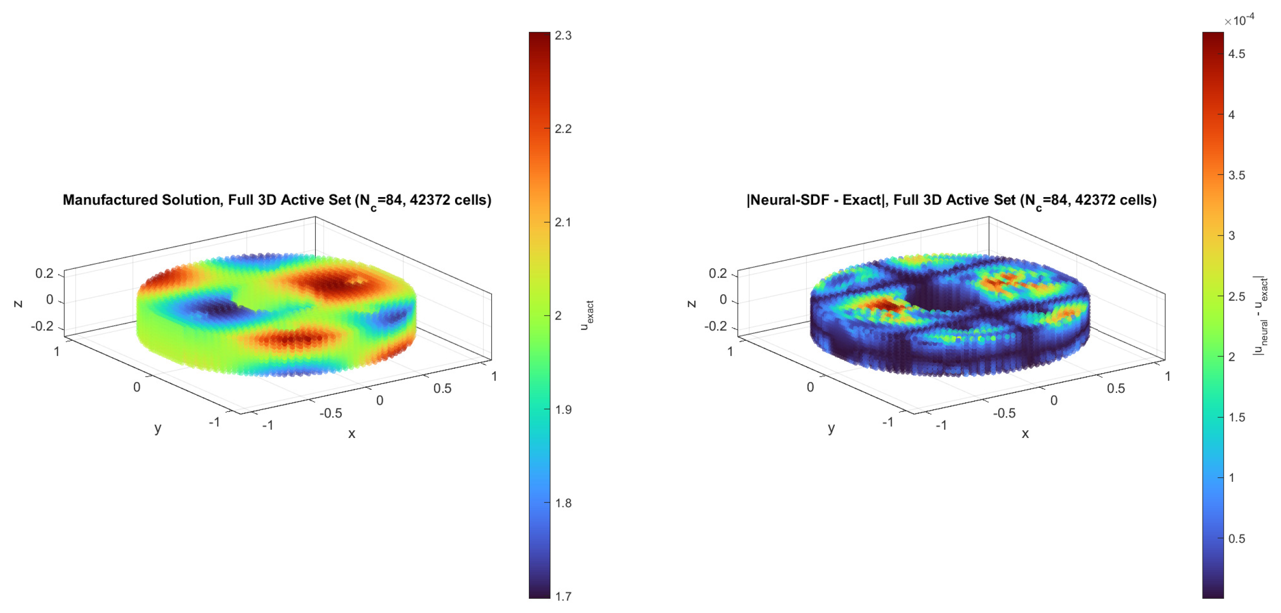
Figure 13 shows the finest-grid discretized domain as a three-dimensional cut-away solid, and Figure 14 shows the corresponding manufactured solution and the neural-SDF pointwise error over the complete three-dimensional active-cell set, rather than a single cross-sectional slice. Repeating neural training at the finest grid over five seeds gives , so run-to-run variability is roughly two orders of magnitude smaller than the error itself, so, exactly as in every two-dimensional example, the neural result does not depend on a favorable seed.
Table 7.
Example 4: regression-based order of accuracy ( vs. , only, grid levels).
Figure 11.
Example 4: manufactured solution and the naive/exact (CSG) / neural-SDF closures on the finest grid (), shown on the cross-section.
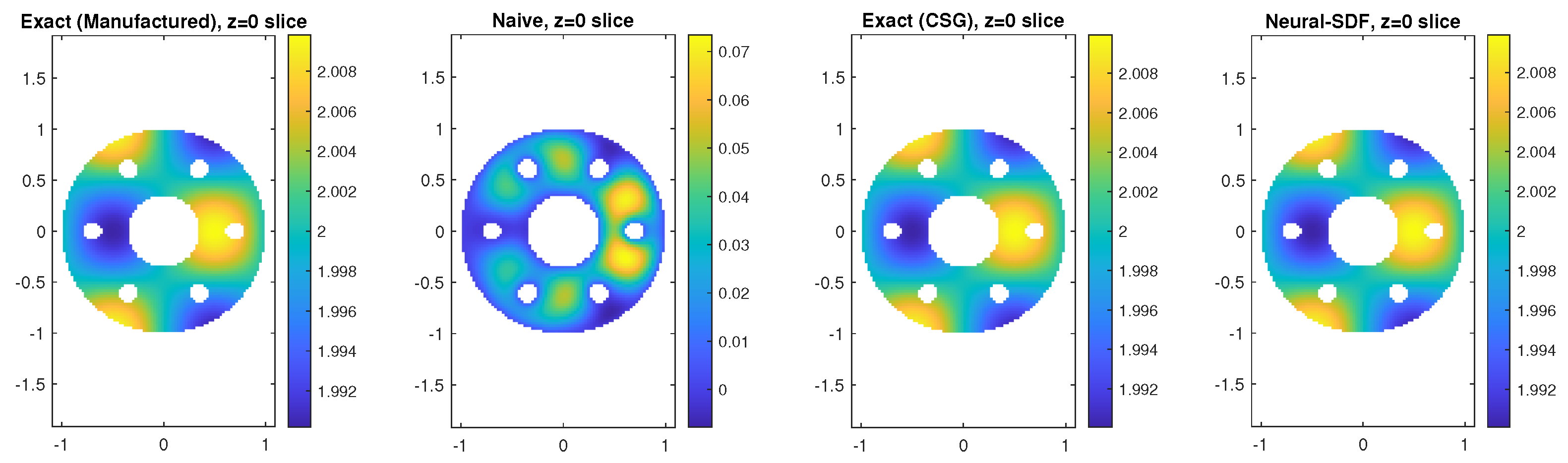
Figure 12.
Example 4: pointwise absolute error, finest grid, cross-section.
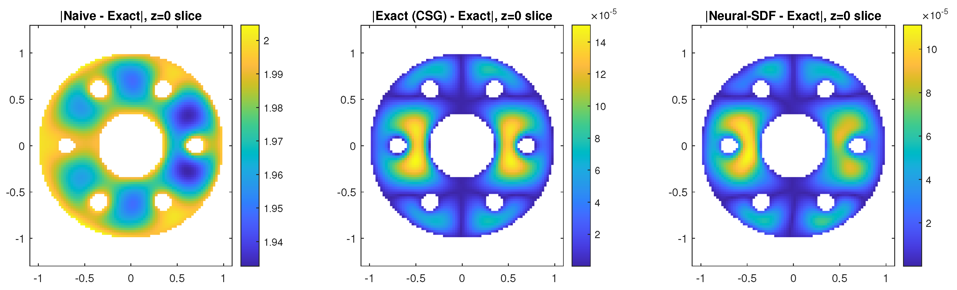
Figure 13.
Example 4: three-dimensional cut-away solid rendering of the mechanical flange domain at the finest grid (), built directly from the solver’s own inside/outside mask rather than a separate idealized drawing. The domain is cut along so the central bore and the near-side bolt holes are visible simultaneously; a faint translucent surface shows the complete, uncut outer envelope for context.
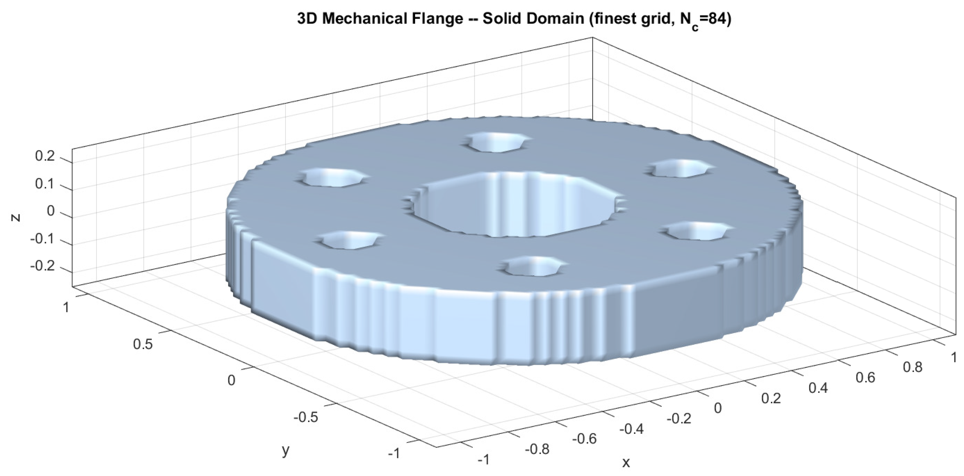
Figure 14.
Example 4: finest-grid () numerical solution rendered over the full three-dimensional active-cell set, not a single cross-sectional slice. Left: the manufactured/exact solution . Right: the pointwise error. Points are drawn with partial transparency so interior structure—the bore and the six bolt holes—remains visible through the outer wall.
5.2. Cost-Scaling
Distance queries against N discrete boundary points are compared across three methods—brute-force linear search ( per query), a KD-tree spatial index ( one-time build, per query), and the trained neural surrogate (fixed network size, per query, independent of N). KD-tree build time is reported as the classical analogue of one-time neural training cost, and KD-tree query time as the analogue of amortized neural query cost; both sides of the ledger are reported, including the regimes where the network does not prevail, and, as elsewhere in this comparison, the resulting crossover points bound the surrogate’s advantage for this specific search-based task rather than for the larger class of costlier calculations it might replace.
Example 1 (flower). Boundary point counts from to were tested (7 repeats per count). At the largest count, brute-force query cost is s/query, KD-tree query (after a one-time s build) is s/query, and the trained network’s batched query cost is s/query, independent of N by construction. The network is thus faster than the KD-tree query and faster than brute force at (Figure 15). The crossover at which the network overtakes the KD-tree query falls in the – point range, visible directly where the constant neural line crosses the KD-tree curve in Figure 15.
Figure 15.
Example 1: query cost vs. boundary point count; brute force vs. KD-tree vs. trained network (fixed cost).
The one-time costs are reported side by side (Figure 16). At the finest grid (), neural-SDF training takes s, versus effectively zero setup cost for the other four closures; per-timestep solve cost is nearly identical across all five (– s/step, 600 steps), so the network’s total cost of s at this problem size is dominated entirely by the one-time training cost. This one-time cost is directly analogous to a KD-tree build and is amortized over however many boundary queries the surrogate subsequently serves, which is precisely why the crossover in Figure 15 favors the network only once N is high enough that this fixed cost is worth paying.
Figure 16.
Example 1: CPU cost breakdown at the finest grid (, 600 timesteps). Per-step solve cost is nearly identical across all five boundary closures; only the neural closure carries a one-time training cost.
Example 2 (multiply-connected domain). Boundary density was scaled by a multiplier from ( points across the outer rim, two holes, and slit) up to ( points), with 7 repeats per density. At maximum density, brute-force query cost is s/query, KD-tree query (after a one-time s build) is s/query, and the network’s batched query cost is s/query, independent of density. The network is thus faster than the KD-tree query and faster than brute force at maximum density (Figure 17). The larger margin relative to Example 1 reflects the larger effective point count needed to resolve six separate boundary components (outer rim, two holes, two slit flanks, slit tip) at comparable per-component resolution. On the one-time side, neural-SDF training at the finest grid takes s (more than Example 1’s training time, consistent with the added geometric complexity), against near-identical per-step solve costs across all five closures (– s/step, 600 steps), giving a total neural cost of s at this problem size.
Figure 17.
Example 2: query cost vs. boundary point count (outer rim, holes, and slit combined); brute force vs. KD-tree vs. trained network.
Example 3 (digitized airfoil). Point-cloud density (resampled from the digitized data) was scaled from to , with 7 repeats per count. At , brute-force query cost is s/query, KD-tree query (after a one-time s build) is s/query, and the network’s batched query cost is s/query, independent of N. The network is thus faster than the KD-tree query and faster than brute force at (Figure 18), consistent with the crossover behavior of Example 1; the constant neural line again crosses the KD-tree curve near – points.
Figure 18.
Example 3: query cost vs. point-cloud density (resampled from the digitized airfoil data); brute force vs. KD-tree vs. trained network.
Example 4 (mechanical flange). Point-cloud density was scaled by resampling the flange’s surface (Section 4.1) from to points (7 repeats per count, as in every other example). At , brute-force query cost is s/query, KD-tree query (after a one-time s build) is s/query, and the network’s batched query cost is s/query, independent of N. The network is thus faster than brute force and faster than the KD-tree query at this density (Figure 19). The crossover at which the network overtakes the KD-tree query falls between , where the KD-tree remains faster ( vs. s/query), and , where the two are already comparable ( s/query)—a somewhat later crossover than the two-dimensional examples’, consistent with three-dimensional KD-tree queries themselves remaining cheap up to higher point counts before the network’s fixed cost wins out.
Figure 19.
Example 4: query cost vs. resampled three-dimensional surface point count; brute force vs. KD-tree vs. trained network.
5.3. Gradient Smoothness
For each example, the outward normal-direction field obtained by finite-differencing the trained neural distance surrogate is compared against the direction to the discrete nearest boundary point (the natural output of a brute-force or KD-tree query), using the total-angular-variation metric of Equation (29) on offset query paths, with the // standoff sensitivity sweep of Section 4.4.
Example 1 (flower). At the base offset, the total angular variation of the normal-direction field is rad for the neural surrogate versus rad for the nearest-point construction, so the nearest-point field carries the variation. This is visible directly in Figure 20, where the neural field’s arrows rotate smoothly along the boundary while the nearest-point field’s arrows flip abruptly near the concave notches between lobes. The ratio is offset-stable, at at the base offset, at , and at —as expected, since moving farther from a fixed set of discrete boundary points reduces how often the nearest-point identity switches, while the neural field remains smooth throughout the entire range tested.
Figure 20.
Example 1: normal-direction field just outside the boundary; neural SDF (left, smooth) vs. nearest-point construction (right, discontinuous near concave notches).
Example 2 (multiply-connected domain). Table 9 breaks the total angular variation down per boundary component. The two smooth circular holes show almost no advantage (–), the outer rim a moderate advantage (), and the reentrant slit the largest advantage among this domain’s boundary components (flanks –; tip ), giving a clean monotone ordering by local geometric severity within a single controlled domain, exactly as predicted by Remark 2. The combined total is ( rad neural vs. rad nearest-point). Figure 21 shows this directly, with the neural normal field rotating smoothly around both holes and along the slit flanks while the nearest-point field is visibly discontinuous entering and exiting the slit. The total ratio is offset-stable, at at the base offset, at , and at .
Table 9.
Example 2: total angular variation (TV) of the normal-direction field, per boundary component, at base offset.
Figure 21.
Example 2: normal-direction field around the multiply-connected boundary; neural SDF (left) vs. nearest-point construction (right, discontinuous at the slit).
Example 3 (digitized airfoil). Total angular variation at the base offset is rad for the neural surrogate versus rad for the nearest-point construction, a ratio—between Example 2’s smooth-hole (≈1×) and reentrant-slit (≈5–) extremes, consistent with a domain that is mostly convex, with no sharp reentrant features but a thin, sharply-curved trailing edge. Figure 22 shows the neural normal field rotating smoothly along the whole airfoil surface, while the nearest-point field flips abruptly near the trailing edge (arc length ), where the identity of the nearest digitized point switches rapidly. The ratio is offset-stable, at at the base offset, at , and at .
Figure 22.
Example 3: normal-direction field along the airfoil surface; neural SDF (left, smooth) vs. nearest-point construction (right, discontinuous near the trailing edge).
Example 4 (mechanical flange). The bore and each bolt hole are surfaces of revolution, so the same one-dimensional angle-unwrap TV construction used in Examples 1 and 2 applies directly at fixed height (Section 4.4); the two flat annular faces use the neighbor mean-angular-difference construction instead. Table 10 breaks the total angular variation down per feature. The outer wall shows the largest advantage of any single feature in this paper (), the bore a substantial one (), and all six bolt holes a smaller, mutually consistent one (–)—and the top face falls in between (). Figure 23 shows this directly for the outer wall and bore, where the neural normal field rotates smoothly while the nearest-point field is visibly discontinuous. The combined ring total is ( rad neural vs. rad nearest-point). The ratio is offset-stable in the same decreasing-with-standoff direction as Examples 1 and 2, with the ring total at at the base offset, at , and at ; the top face likewise falls from to to (the sweep’s face value differs slightly from Table 10’s because the face sample points are drawn independently at random for each measurement).
Table 10.
Example 4: total angular variation (TV) of the normal-direction field, per boundary feature, at base offset. Ring features (outer wall, bore, bolt holes) use the angle-unwrap TV construction; the top face uses the mean neighbor-angular-difference construction (units rad, not directly comparable in scale to the TV rows).
Figure 23.
Example 4: normal-direction field on the outer wall ring; neural SDF (left, smooth) vs. nearest-point construction (right, discontinuous).
This ordering is worth stating plainly, because it does not match Example 2’s pattern. There, smoothness advantage tracked concavity, and the smooth round holes showed almost no advantage (–) and the sharp reentrant slit showed the most (5–). Here, the bore—a smooth round hole, geometrically the same kind of feature as Example 2’s holes—shows a much larger advantage () than the bolt holes (–), which are the tightest-curvature, most concave features on this part. The ordering instead tracks feature radius, with the outer wall () showing the largest ratio, the bore () an intermediate one, and the bolt holes (, the smallest) the smallest and most mutually consistent ratios, as summarized directly by the per-feature smoothness ratios of Figure 24. The most likely explanation is a point-cloud-density effect rather than a concavity effect, since the reference cloud used throughout this example is allocated in proportion to patch area, giving every ring the same areal point density regardless of radius, but a fixed areal density still yields more absolute points, and finer angular resolution at a fixed offset, on a larger ring than a smaller one. A clean separation of the concavity effect documented in Example 2 from this radius/density effect would require matching linear (arc-length) rather than areal point density across features of different size, which this experiment did not control for and is left as an open question rather than folded into a single explanation. It does not change the paper’s central smoothness claim—the neural field is smoother than the nearest-point construction at every feature and every offset tested, here as in every other example—only the specific claim that the advantage is driven by concavity alone. Formalizing this distinction–isolating the sampling-density contribution from the concavity contribution to the smoothness ratio, and establishing whether an arc-length-proportional point allocation removes the radius dependence observed here–constitutes a natural open question for future gradient-smoothness studies of this kind, distinct from the concavity mechanism established analytically in Remark 2 and confirmed in two dimensions.
Figure 24.
Example 4: smoothness ratio (nearest-point TV/neural TV) by feature, showing the ordering by radius (outer wall > bore > bolt holes) rather than by concavity.
6. Conclusions
This work investigated whether a compact neural network can serve as an accurate and efficient surrogate for the signed distance function within an otherwise unchanged cut-cell finite-volume framework, a question distinct from the growing literature on learned distance fields as an auxiliary component of a larger neural architecture (Section 2): here the distance function alone is substituted into a conventional, unmodified solver, and the numerical consequences of that substitution—rather than end-to-end model accuracy—are what is assessed. The proposed approach was evaluated on four benchmark problems spanning analytical and digitized geometries in both two and three spatial dimensions, with the assessment structured around three complementary questions: numerical accuracy, computational cost, and gradient smoothness.
The verification studies demonstrate that replacing the exact signed distance function with the neural surrogate preserves the formal second-order accuracy of the underlying discretization. Across all benchmark problems, the measured convergence rates are statistically consistent with the theoretical prediction established in Proposition 1, confirming that the surrogate satisfies the near-boundary accuracy requirement identified in Remark 1. The wider confidence interval observed for the three-dimensional benchmark is explained by mesh-resolution and temporal discretization effects that influence both the exact and neural closures, rather than by limitations of the surrogate itself.
From a computational perspective, the neural surrogate exhibits the expected constant-cost evaluation independent of boundary complexity. While classical KD-tree searches remain more efficient for modest point-cloud sizes, the surrogate becomes increasingly advantageous as the geometric representation is refined, ultimately providing substantial speedups for large-scale boundary datasets. These results indicate that the proposed approach is most beneficial in applications where highly resolved or repeatedly queried geometries make distance evaluation a significant computational bottleneck.
The study also demonstrates a consistent qualitative advantage of the neural representation over discrete nearest-point constructions. In every benchmark, the learned signed distance field produces a smoother and continuously differentiable gradient field, yielding more regular boundary normals without compromising numerical accuracy. Although the magnitude of this advantage depends on local geometric characteristics, the improvement is observed consistently across all geometries and spatial dimensions considered.
Overall, the results show that a compact, grid-specific neural signed distance surrogate can replace exact geometric distance evaluations in cut-cell finite-volume discretizations without sacrificing accuracy, while offering improved gradient smoothness and favorable computational scaling for sufficiently complex geometries. More broadly, the work demonstrates that learning the geometric representation, rather than modifying the numerical discretization itself, provides an effective pathway for integrating machine learning into established PDE solvers while preserving their theoretical properties.
Several directions remain for future work. These include extending the three-dimensional verification to scan-derived geometries lacking analytical descriptions, investigating the influence of feature scale and sampling density on gradient smoothness, comparing alternative neural representations such as periodic-activation or encoded networks, KAN and Wav-KAN, or higher-order wavelet-network surrogates [33,34,35] within the same evaluation framework, and applying the approach to nonlinear or moving-boundary problems, where the availability of smooth, differentiable geometric information may be more valuable than reductions in query cost alone, though a genuinely moving boundary raises a difficulty not addressed by the present study: every result reported here retrains the network from scratch at a fixed geometry, amortizing that one-time cost across many subsequent queries, and a moving boundary would need an online or incremental update scheme rather than full retraining at every time step for the approach to remain computationally viable.
Author Contributions
Conceptualization, A.Q. and S.O.; methodology, A.Q. and S.O.; software, A.Q. and S.O.; validation, A.Q. and S.O.; formal analysis, A.Q. and S.O.; investigation, A.Q. and S.O.; resources, A.Q. and S.O.; data curation, A.Q. and S.O.; writing—original draft preparation, A.Q. and S.O.; writing—review and editing, A.Q. and S.O.; visualization, A.Q. and S.O. All authors have read and agreed to the published version of the manuscript.
Funding
This research received no external funding.
Data Availability Statement
The raw data supporting the conclusions of this article will be made available by the authors on request.
Acknowledgments
The authors gratefully acknowledge the support and valuable discussions provided by the members of the Engineering Model and Design (E-MoDe) Research Group (RG-BU008) and the Engineering Computation and Intelligence (ECI) Research Group (RG-BU006), both supported by the Deanship of Graduate Studies and Scientific Research at Bethlehem University. During the preparation of this manuscript, the authors used Claude (Anthropic) for the purposes of improving the language, wording, and clarity of the manuscript. The authors have reviewed and edited the output and take full responsibility for the content of this publication.
Conflicts of Interest
The authors declare no conflicts of interest.
References
- Peskin, C.S. Flow patterns around heart valves: A numerical method. J. Comput. Phys. 1972, 10, 252–271. [Google Scholar] [CrossRef] [Scilit]
- Peskin, C.S. Numerical analysis of blood flow in the heart. J. Comput. Phys. 1977, 25, 220–252. [Google Scholar] [CrossRef] [Scilit]
- Peskin, C.S. The immersed boundary method. Acta Numer. 2002, 11, 479–517. [Google Scholar] [CrossRef] [Scilit]
- Mittal, R.; Iaccarino, G. Immersed boundary methods. Annu. Rev. Fluid Mech. 2005, 37, 239–261. [Google Scholar] [CrossRef] [Scilit]
- Johansen, H.; Colella, P. A Cartesian grid embedded boundary method for Poisson’s equation on irregular domains. J. Comput. Phys. 1998, 147, 60–85. [Google Scholar] [CrossRef] [Scilit]
- Fedkiw, R.P.; Aslam, T.; Merriman, B.; Osher, S. A non-oscillatory Eulerian approach to interfaces in multimaterial flows (the ghost fluid method). J. Comput. Phys. 1999, 152, 457–492. [Google Scholar] [CrossRef] [Scilit]
- Gibou, F.; Fedkiw, R.P.; Cheng, L.T.; Kang, M. A second-order-accurate symmetric discretization of the Poisson equation on irregular domains. J. Comput. Phys. 2002, 176, 205–227. [Google Scholar] [CrossRef] [Scilit]
- Yang, T.; Qarariyah, A.; Deng, J. Spline R-function and applications in FEM. Numer. Math. Theory Methods Appl. 2020, 13, 150–175. [Google Scholar] [CrossRef] [Scilit]
- Qarariyah, A.; Yang, T.; Deng, F. A Solution-Structure B-Spline-Based Framework for Hybrid Boundary Problems on Implicit Domains. Mathematics 2024, 12, 3973. [Google Scholar] [CrossRef] [Scilit]
- Sethian, J.A. Level Set Methods and Fast Marching Methods: Evolving Interfaces in Computational Geometry, Fluid Mechanics, Computer Vision, and Materials Science; Cambridge University Press: Cambridge, UK, 1999. [Google Scholar]
- Belyaev, A.G.; Fayolle, P.A. On variational and PDE-based distance function approximations. Proc. Comput. Graph. Forum 2015, 34, 104–118. [Google Scholar] [CrossRef] [Scilit]
- Bentley, J.L. Multidimensional binary search trees used for associative searching. Commun. ACM 1975, 18, 509–517. [Google Scholar] [CrossRef] [Scilit]
- Friedman, J.H.; Bentley, J.L.; Finkel, R.A. An algorithm for finding best matches in logarithmic expected time. ACM Trans. Math. Softw. 1977, 3, 209–226. [Google Scholar] [CrossRef] [Scilit]
- Curless, B.; Levoy, M. A volumetric method for building complex models from range images. In Proceedings of the 23rd Annual Conference on Computer Graphics and Interactive Techniques (SIGGRAPH), New Orleans, LA, USA, 4–9 August 1996; pp. 303–312. [Google Scholar]
- Kazhdan, M.; Bolitho, M.; Hoppe, H. Poisson surface reconstruction. In Proceedings of the Fourth Eurographics Symposium on Geometry Processing, Cagliari, Sardinia, Italy, 26–28 June 2006; pp. 61–70. [Google Scholar]
- Selig, M.S.; Guglielmo, J.J.; Broeren, A.P.; Giguère, P. Summary of Low-Speed Airfoil Data; SoarTech Publications: Virginia Beach, VA, USA, 1995; Volume 1. [Google Scholar]
- Selig, M.S. UIUC Airfoil Coordinates Database. 1996. Available online: https://m-selig.ae.illinois.edu/ads/coord_database.html (accessed on 19 August 2026).
- Park, J.J.; Florence, P.; Straub, J.; Newcombe, R.; Lovegrove, S. DeepSDF: Learning continuous signed distance functions for shape representation. In Proceedings of the IEEE/CVF Conference on Computer Vision and Pattern Recognition (CVPR), Long Beach, CA, USA, 16–19 June 2019; pp. 165–174. [Google Scholar]
- Mescheder, L.; Oechsle, M.; Niemeyer, M.; Nowozin, S.; Geiger, A. Occupancy networks: Learning 3D reconstruction in function space. In Proceedings of the IEEE/CVF Conference on Computer Vision and Pattern Recognition (CVPR), Long Beach, CA, USA, 16–19 June 2019; pp. 4460–4470. [Google Scholar]
- Mildenhall, B.; Srinivasan, P.P.; Tancik, M.; Barron, J.T.; Ramamoorthi, R.; Ng, R. NeRF: Representing scenes as neural radiance fields for view synthesis. In Proceedings of the European Conference on Computer Vision (ECCV), Glasgow, UK, 23–28 August 2020; pp. 405–421. [Google Scholar]
- Rahaman, N.; Baratin, A.; Arpit, D.; Draxler, F.; Lin, M.; Hamprecht, F.; Bengio, Y.; Courville, A. On the spectral bias of neural networks. In Proceedings of the 36th International Conference on Machine Learning, Long Beach, CA, USA, 9–15 June 2019; Volume 97, pp. 5301–5310, Proceedings of Machine Learning Research. [Google Scholar]
- Tancik, M.; Srinivasan, P.; Mildenhall, B.; Fridovich-Keil, S.; Raghavan, N.; Singhal, U.; Ramamoorthi, R.; Barron, J.; Ng, R. Fourier features let networks learn high frequency functions in low dimensional domains. Proc. Adv. Neural Inf. Process. Syst. 2020, 33, 7537–7547. [Google Scholar]
- Sitzmann, V.; Martel, J.; Bergman, A.; Lindell, D.; Wetzstein, G. Implicit neural representations with periodic activation functions. Proc. Adv. Neural Inf. Process. Syst. 2020, 33, 7462–7473. [Google Scholar]
- Lagaris, I.E.; Likas, A.; Fotiadis, D.I. Artificial neural networks for solving ordinary and partial differential equations. IEEE Trans. Neural Netw. 1998, 9, 987–1000. [Google Scholar] [CrossRef] [Scilit]
- Qarariyah, A.; Yang, T.; Deng, F. An Intelligent SPH Framework Based on Machine-Learned Residual Correction for Elliptic PDEs. Algorithms 2025, 18, 803. [Google Scholar] [CrossRef] [Scilit]
- Raissi, M.; Perdikaris, P.; Karniadakis, G.E. Physics-informed neural networks: A deep learning framework for solving forward and inverse problems involving nonlinear partial differential equations. J. Comput. Phys. 2019, 378, 686–707. [Google Scholar] [CrossRef] [Scilit]
- Sukumar, N.; Srivastava, A. Exact imposition of boundary conditions with distance functions in physics-informed deep neural networks. Comput. Methods Appl. Mech. Eng. 2022, 389, 114333. [Google Scholar] [CrossRef] [Scilit]
- Gao, H.; Sun, L.; Wang, J.X. PhyGeoNet: Physics-informed geometry-adaptive convolutional neural networks for solving parameterized steady-state PDEs on irregular domain. J. Comput. Phys. 2021, 428, 110079. [Google Scholar] [CrossRef] [Scilit]
- Oldenburg, J.; Borowski, F.; Öner, A.; Schmitz, K.P.; Stiehm, M. Geometry aware physics informed neural network surrogate for solving Navier–Stokes equation (GAPINN). Adv. Model. Simul. Eng. Sci. 2022, 9, 8. [Google Scholar] [CrossRef] [Scilit]
- Li, Z.; Kovachki, N.B.; Choy, C.; Li, B.; Kossaifi, J.; Otta, S.P.; Nabian, M.A.; Stadler, M.; Hundt, C.; Azizzadenesheli, K.; et al. Geometry-informed neural operator for large-scale 3D PDEs. Proc. Adv. Neural Inf. Process. Syst. 2023, 36, 35836–35854. [Google Scholar] [CrossRef] [Scilit]
- Rabeh, A.; Krishnamurthy, A.; Ganapathysubramanian, B. 3D neural operator-based flow surrogates around 3D geometries: Signed distance functions and derivative constraints. arXiv 2025, arXiv:2503.17289. [Google Scholar]
- Zhang, L.; Pagani, S.; Zhang, J.; Regazzoni, F. Shape-informed surrogate models based on signed distance function domain encoding. J. Comput. Phys. 2025, 538, 114178. [Google Scholar] [CrossRef] [Scilit]
- Liu, Z.; Wang, Y.; Vaidya, S.; Ruehle, F.; Halverson, J.; Soljačić, M.; Hou, T.Y.; Tegmark, M. KAN: Kolmogorov–Arnold Networks. arXiv 2024, arXiv:2404.19756. [Google Scholar]
- Bozorgasl, Z.; Chen, H. Wav-KAN: Wavelet Kolmogorov–Arnold Networks. arXiv 2024, arXiv:2405.12832. [Google Scholar]
- Majak, J.; Pohlak, M.; Karjust, K.; Eerme, M.; Kurnitski, J.; Shvartsman, B. New Higher Order Haar Wavelet Method: Application to FGM Structures. Compos. Struct. 2018, 201, 72–78. [Google Scholar] [CrossRef] [Scilit]
- Roache, P.J. Code verification by the method of manufactured solutions. J. Fluids Eng. 2002, 124, 4–10. [Google Scholar] [CrossRef] [Scilit]
- Aycock, K.I.; Rebelo, N.; Craven, B.A. Method of Manufactured Solutions Code Verification of Elastostatic Solid Mechanics Problems in a Commercial Finite Element Solver. Comput. Math. Appl. 2021, 93, 178–198. [Google Scholar]
- Gibou, F.; Fedkiw, R.; Osher, S. A review of level-set methods and some recent applications. J. Comput. Phys. 2018, 353, 82–109. [Google Scholar] [CrossRef] [Scilit]
- Ascher, U.M.; Ruuth, S.J.; Wetton, B.T.R. Implicit-explicit methods for time-dependent partial differential equations. SIAM J. Numer. Anal. 1995, 32, 797–823. [Google Scholar] [CrossRef] [Scilit]
- Hu, J.; Shu, R. Uniform Accuracy of Implicit-Explicit Runge–Kutta (IMEX-RK) Schemes for Hyperbolic Systems with Relaxation. Math. Comput. 2024, 94, 209–240. [Google Scholar] [CrossRef] [Scilit]
- Shortley, G.H.; Weller, R. The numerical solution of Laplace’s equation. J. Appl. Phys. 1938, 9, 334–348. [Google Scholar] [CrossRef] [Scilit]
- Berger, M. Cut cells: Meshes and solvers. In Handbook of Numerical Methods for Hyperbolic Problems; Handbook of Numerical Analysis; Elsevier: Amsterdam, The Netherlands, 2017; Volume 18, pp. 1–22. [Google Scholar]
- Gulizzi, V.; Almgren, A.S.; Bell, J.B. A Coupled Discontinuous Galerkin-Finite Volume Framework for Solving Gas Dynamics over Embedded Geometries. J. Comput. Phys. 2022, 450, 110861. [Google Scholar] [CrossRef] [Scilit]
- Berger, M.; Giuliani, A. A State Redistribution Algorithm for Finite Volume Schemes on Cut Cell Meshes. J. Comput. Phys. 2021, 428, 109820. [Google Scholar] [CrossRef] [Scilit]
- Ram, P.; Sinha, K. Revisiting kd-tree for Nearest Neighbor Search. In Proceedings of the 25th ACM SIGKDD International Conference on Knowledge Discovery & Data Mining (KDD), Anchorage, AK, USA, 4–8 August 2019; pp. 1378–1388. [Google Scholar]
- Aumüller, M.; Ceccarello, M. Recent Approaches and Trends in Approximate Nearest Neighbor Search, with Remarks on Benchmarking. IEEE Data Eng. Bull. 2023, 46, 89–105. [Google Scholar]
- Aurenhammer, F. Voronoi diagrams—A survey of a fundamental geometric data structure. ACM Comput. Surv. 1991, 23, 345–405. [Google Scholar] [CrossRef] [Scilit]
- Cybenko, G. Approximation by superpositions of a sigmoidal function. Math. Control Signals Syst. 1989, 2, 303–314. [Google Scholar] [CrossRef] [Scilit]
- Hornik, K. Approximation capabilities of multilayer feedforward networks. Neural Netw. 1991, 4, 251–257. [Google Scholar] [CrossRef] [Scilit]
- Augustine, M.T. A Survey on Universal Approximation Theorems. arXiv 2024, arXiv:2407.12895. [Google Scholar]
- Worth, K.; Plamus, T.; Majak, J. Design optimization of nonwovens made from mechanically recycled textile fibres. Compos. Struct. 2026, 387, 120330. [Google Scholar] [CrossRef] [Scilit]
- Levenberg, K. A method for the solution of certain non-linear problems in least squares. Q. Appl. Math. 1944, 2, 164–168. [Google Scholar] [CrossRef] [Scilit]
- Marquardt, D.W. An algorithm for least-squares estimation of nonlinear parameters. J. Soc. Ind. Appl. Math. 1963, 11, 431–441. [Google Scholar] [CrossRef] [Scilit]
- Hagan, M.T.; Menhaj, M.B. Training feedforward networks with the Marquardt algorithm. IEEE Trans. Neural Netw. 1994, 5, 989–993. [Google Scholar] [CrossRef] [Scilit]
- Møller, M.F. A scaled conjugate gradient algorithm for fast supervised learning. Neural Netw. 1993, 6, 525–533. [Google Scholar] [CrossRef] [Scilit]
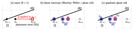
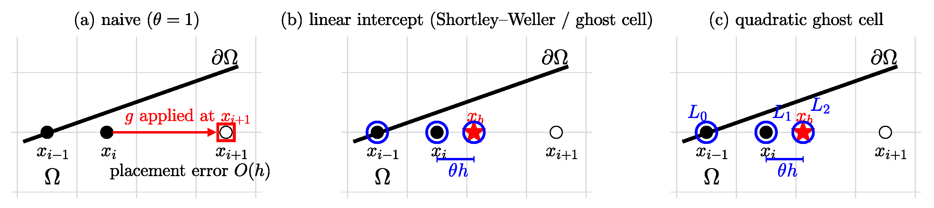
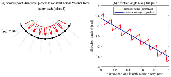
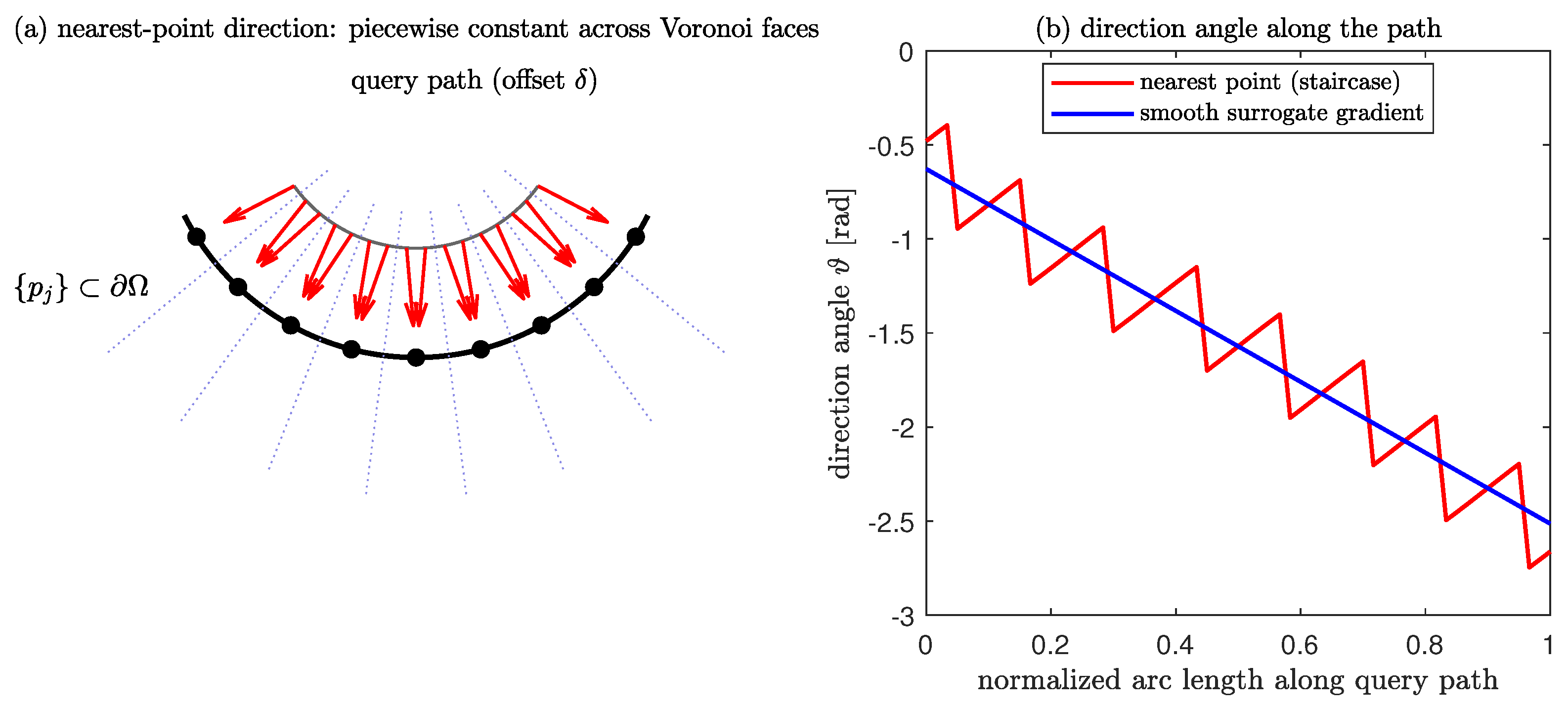
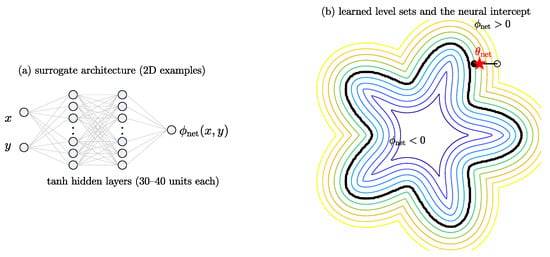
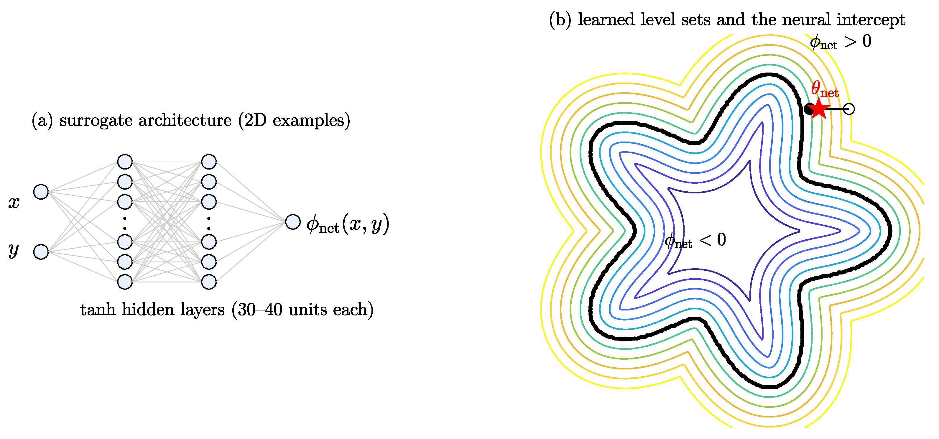
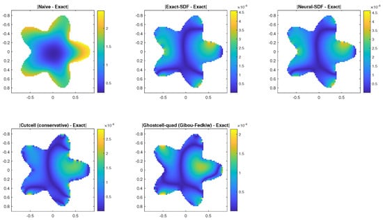
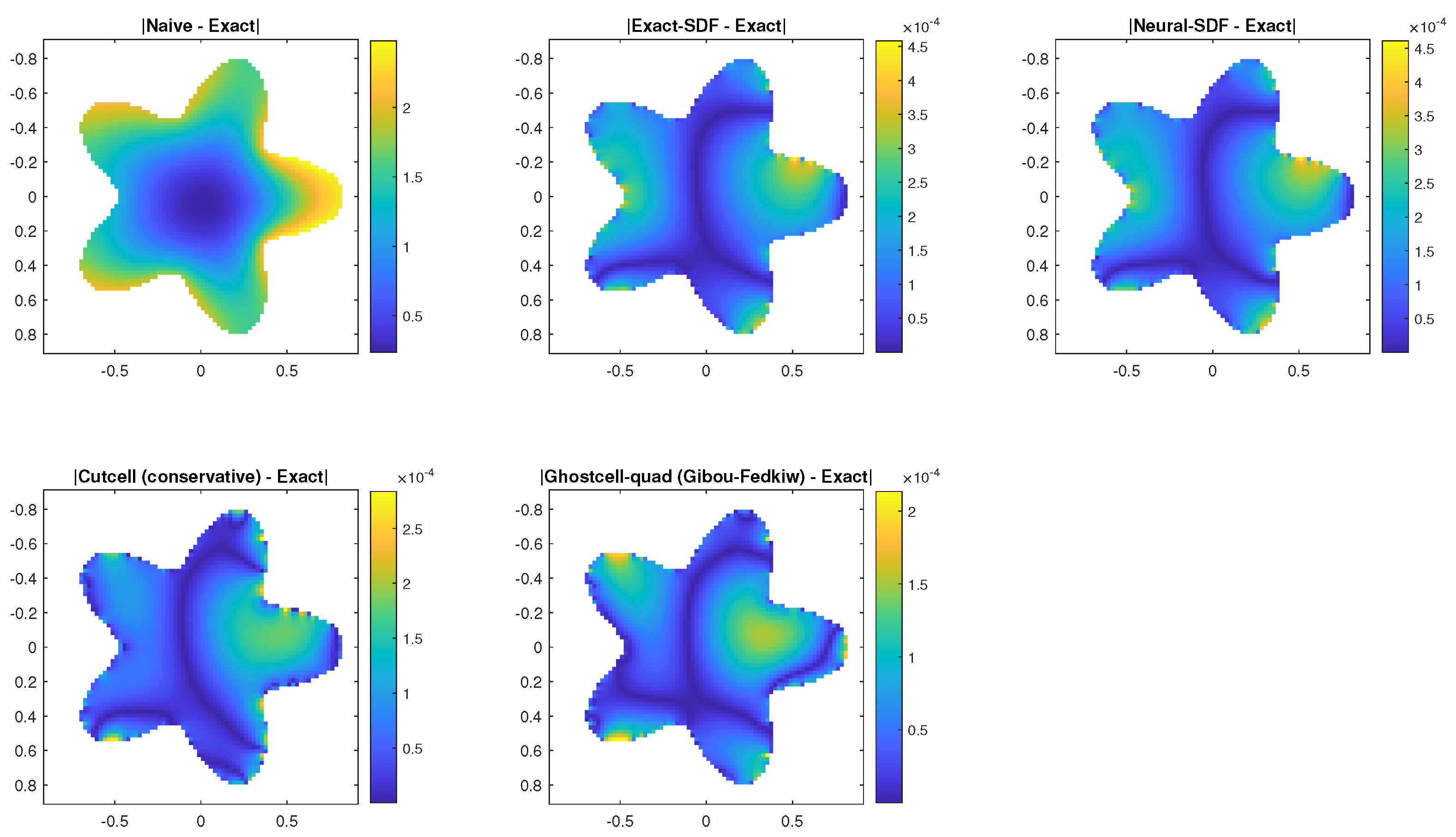
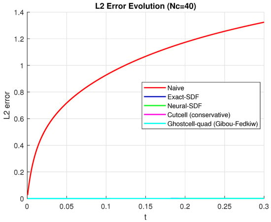
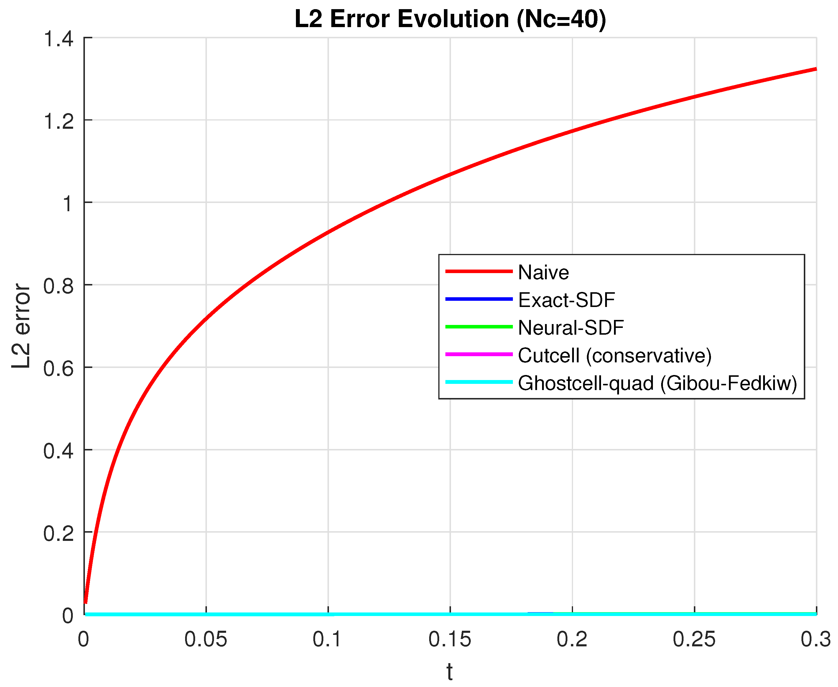
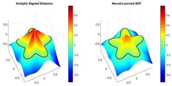
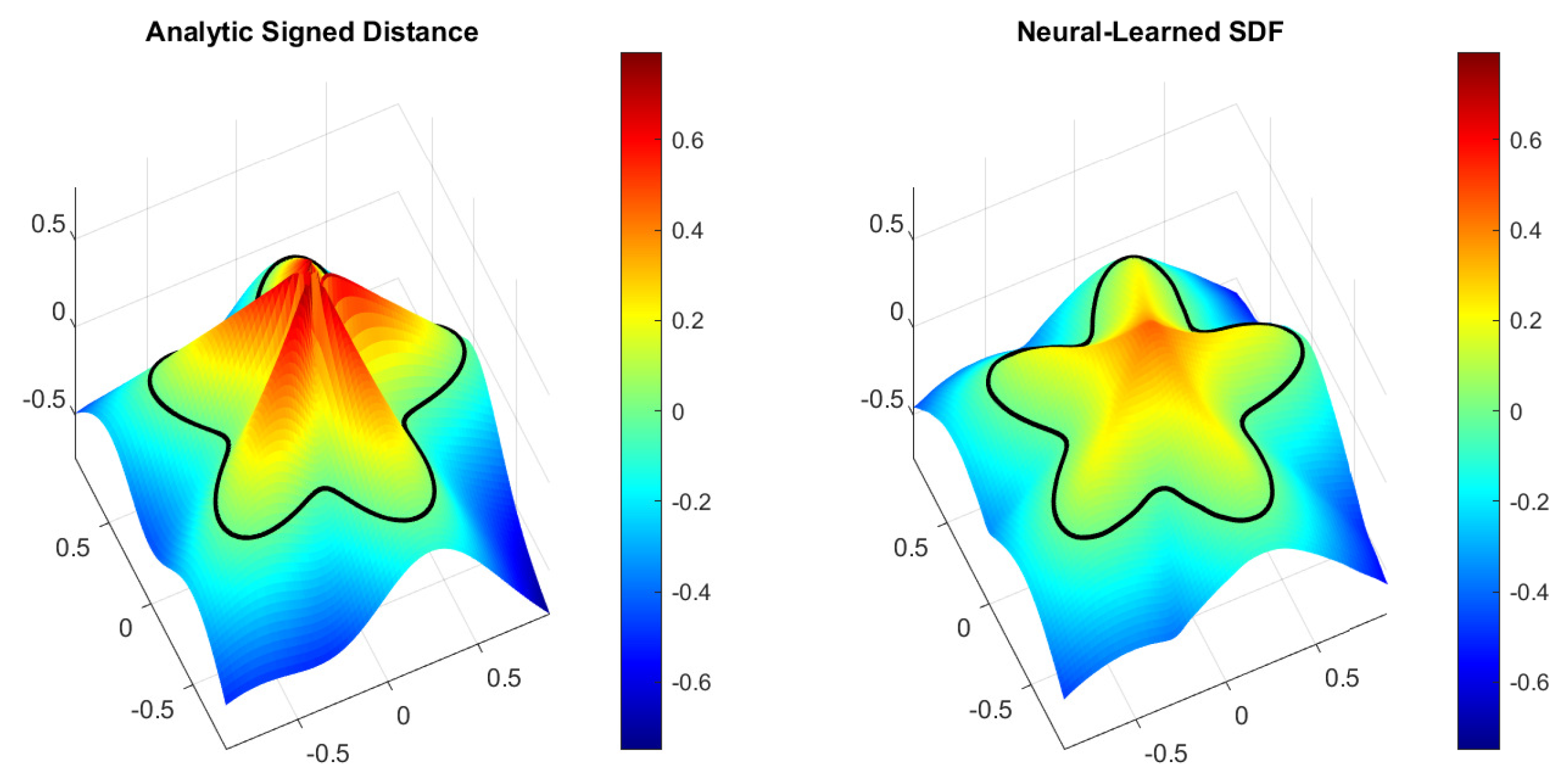
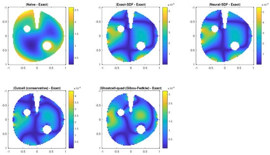
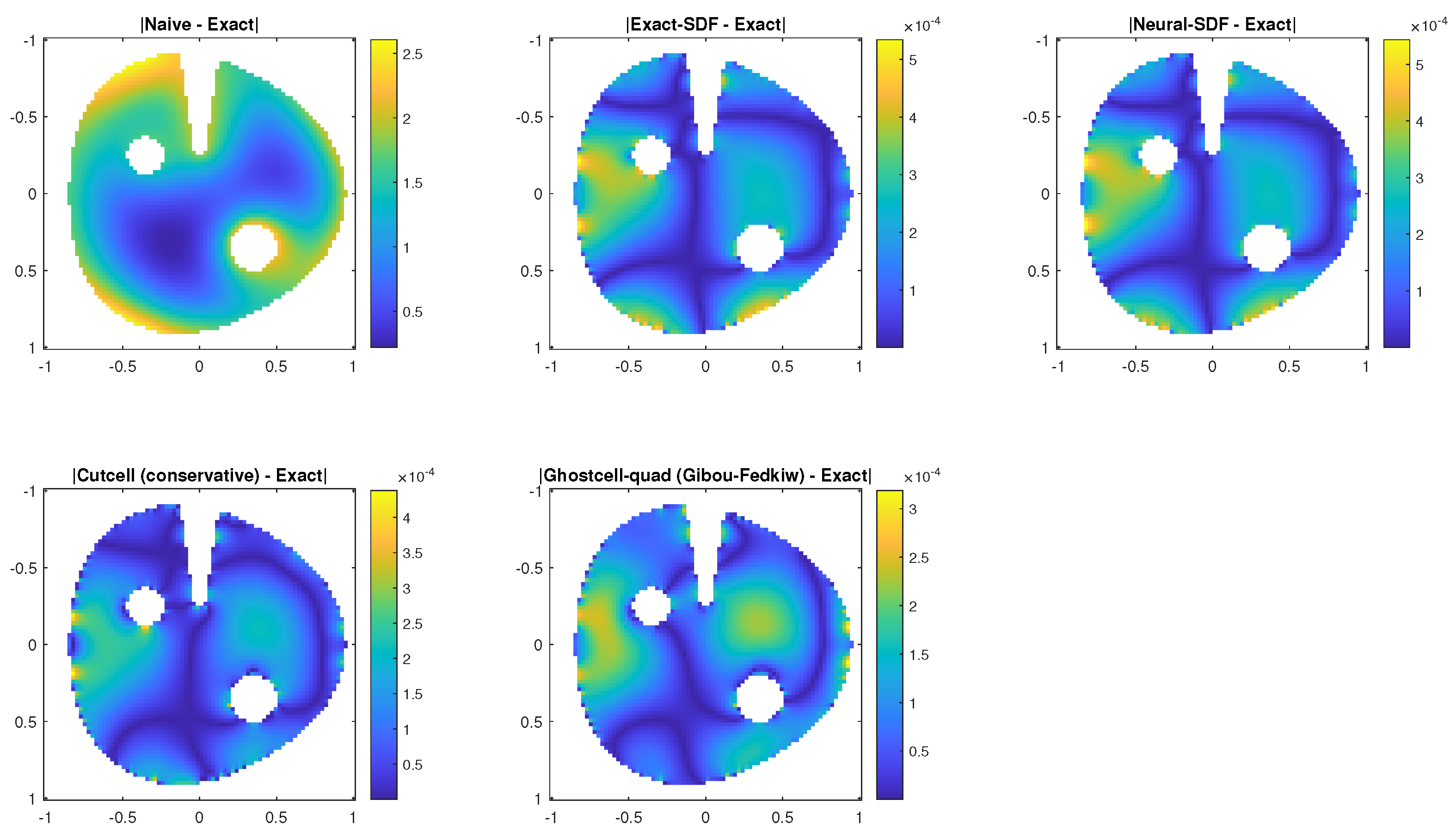
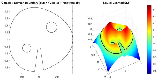
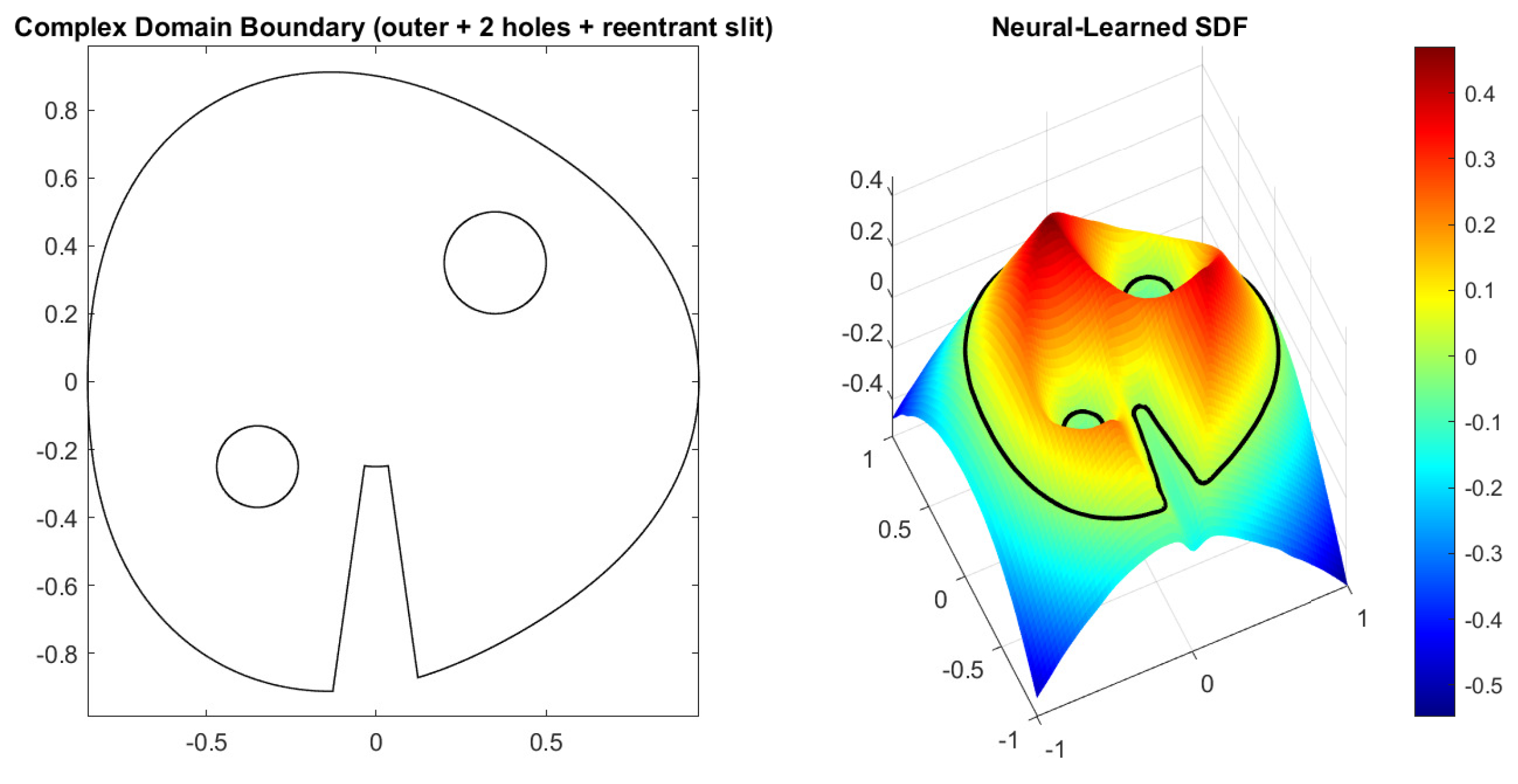
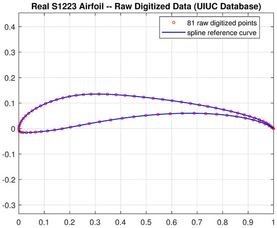
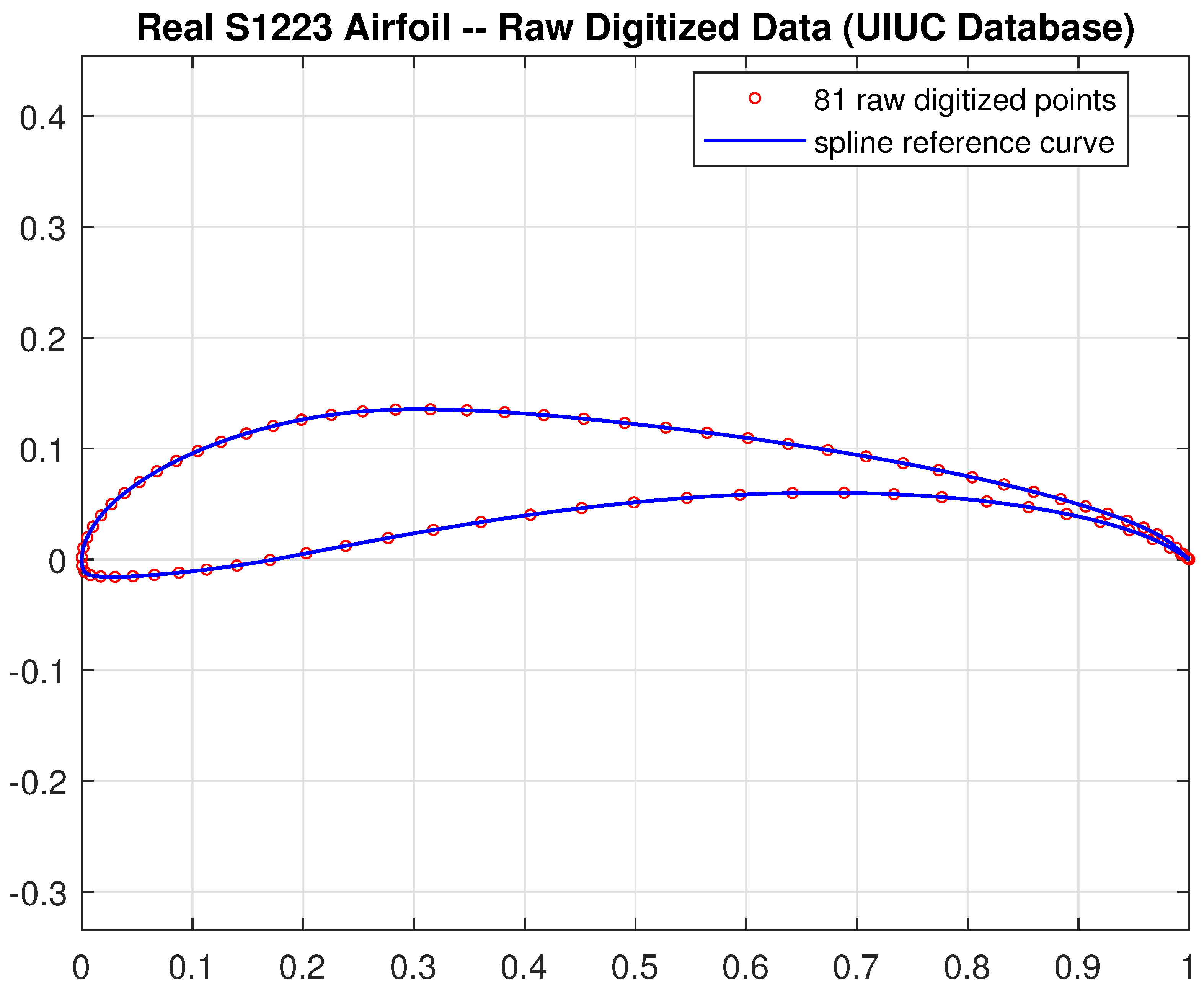
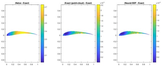
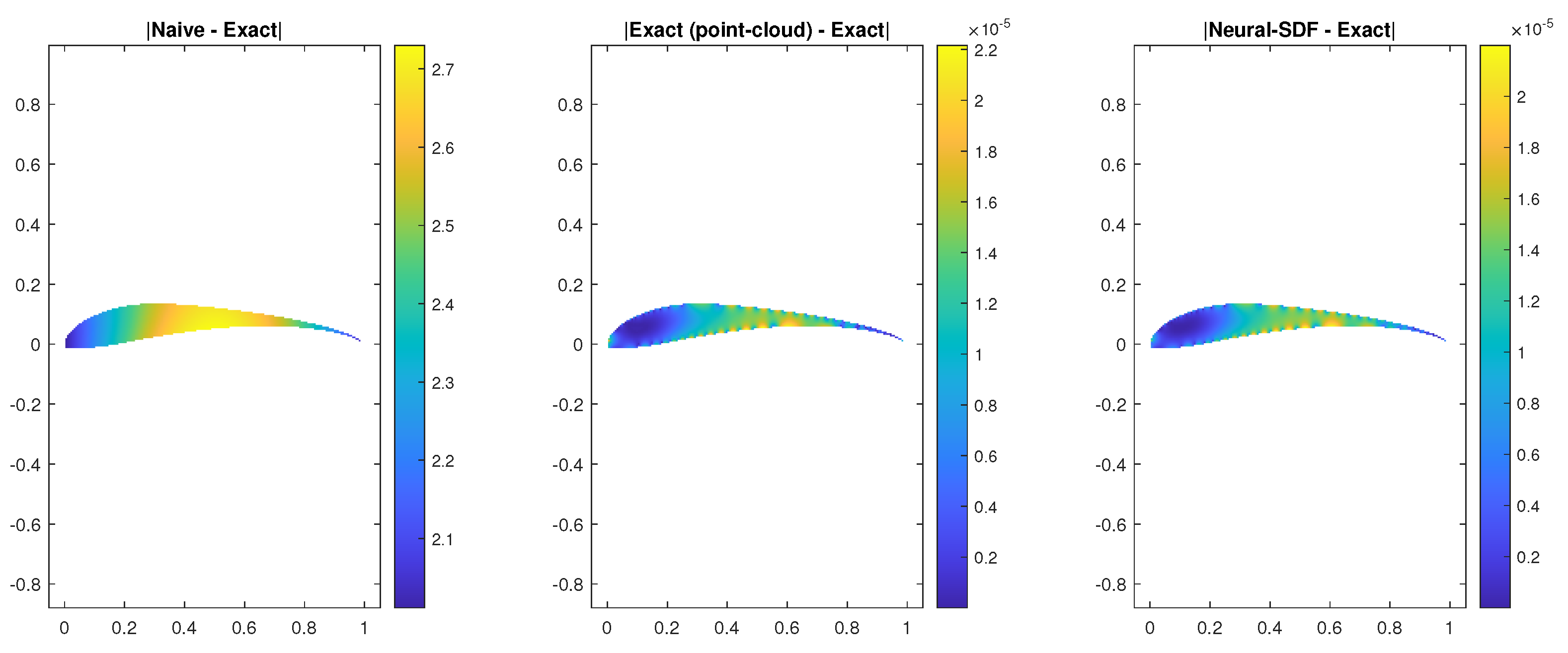
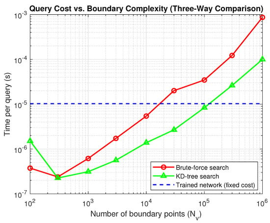
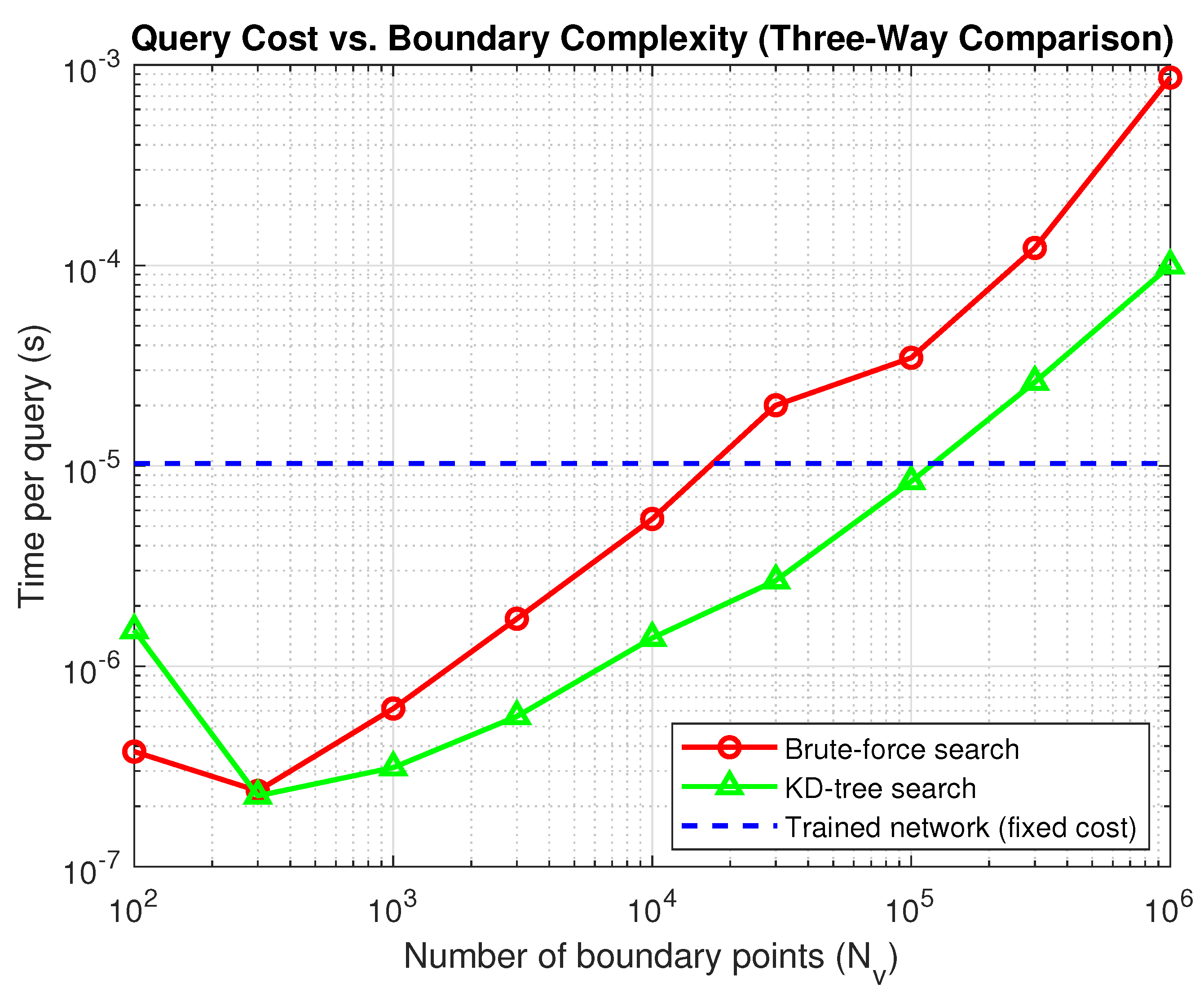
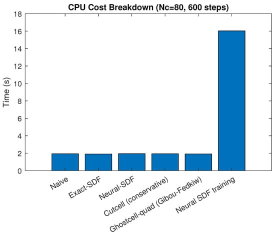
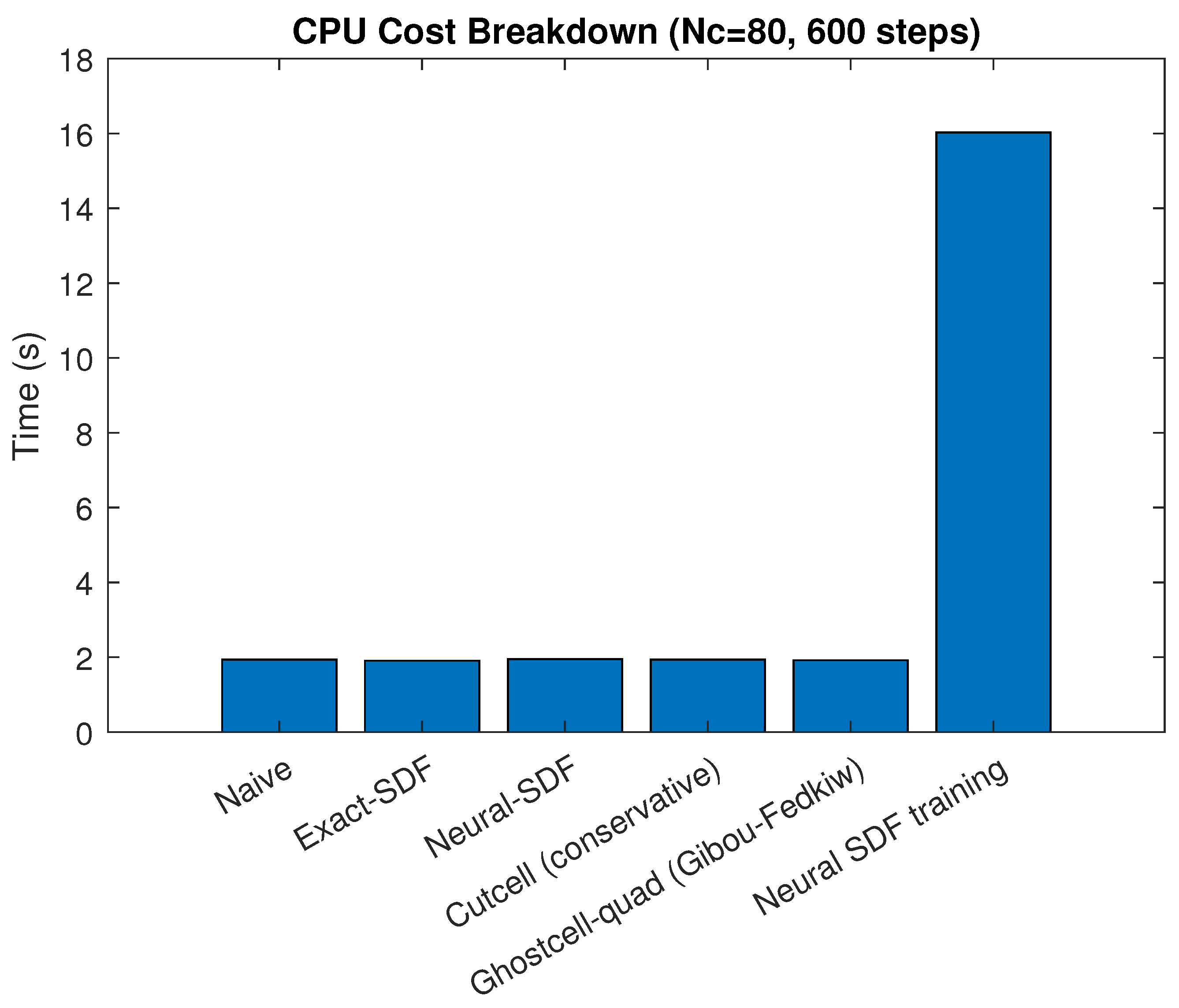
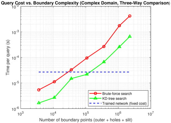
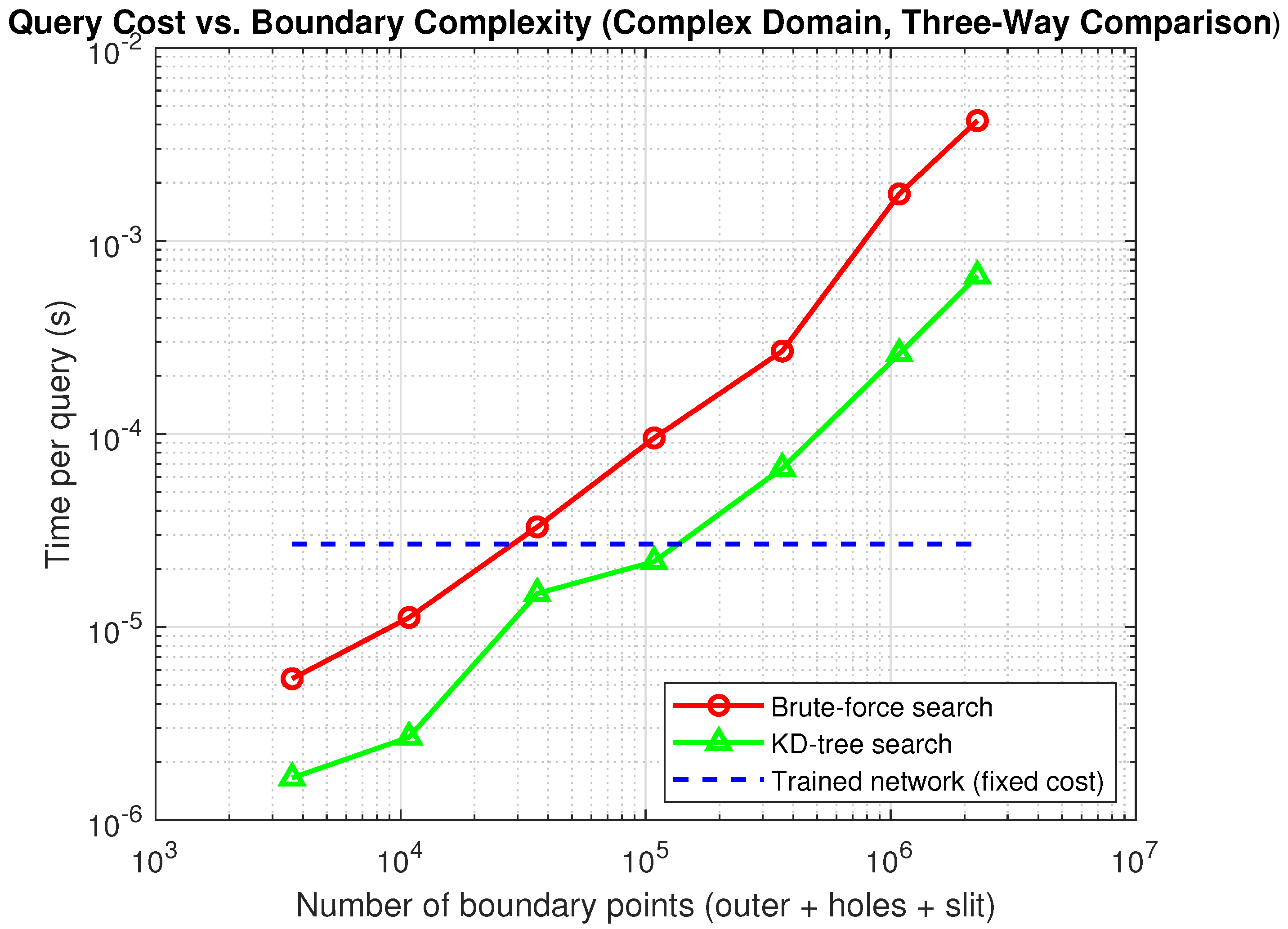
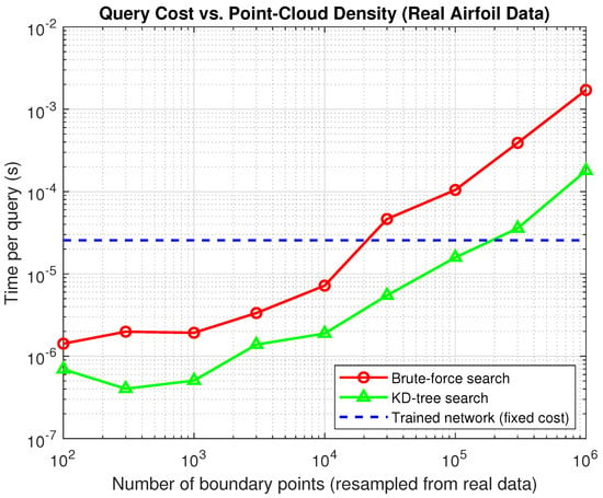
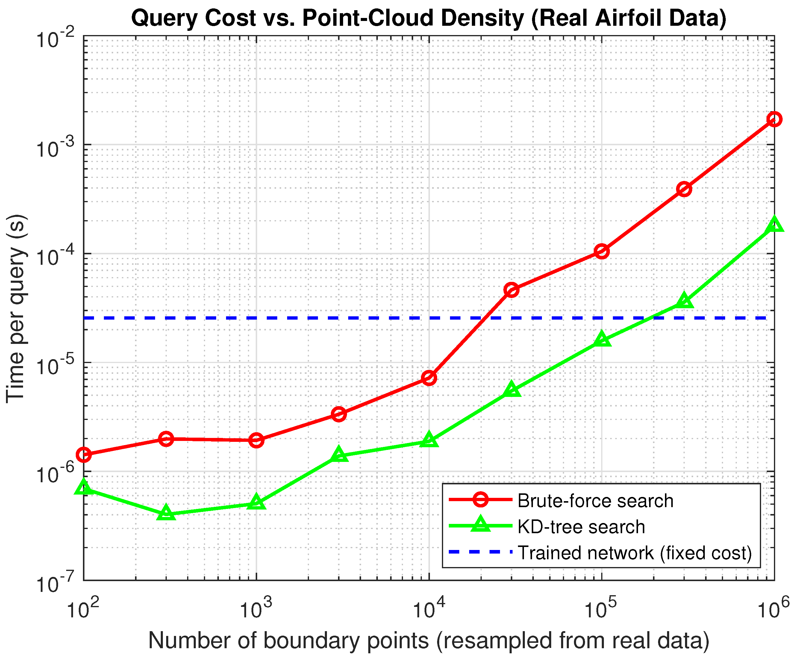
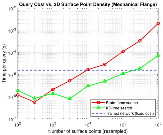
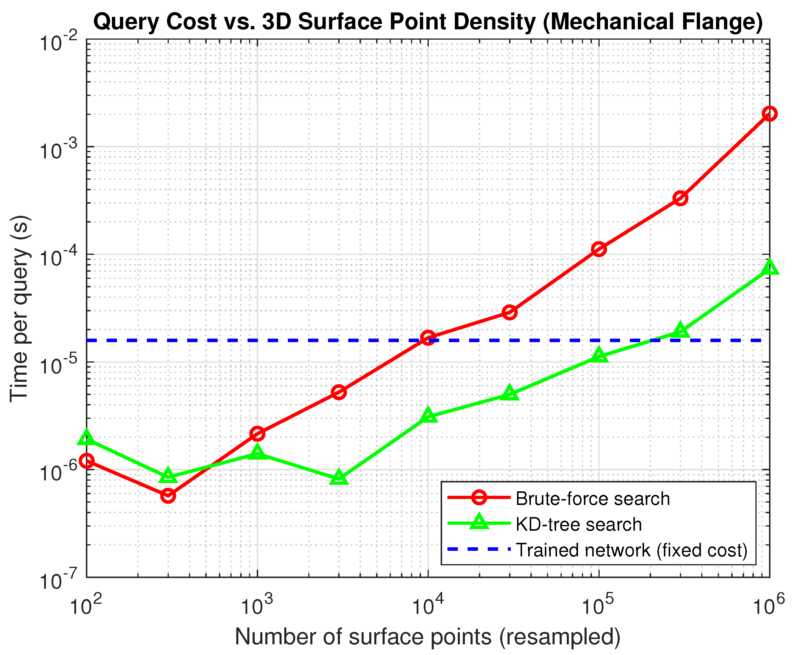
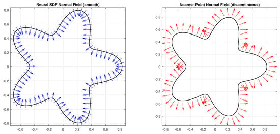
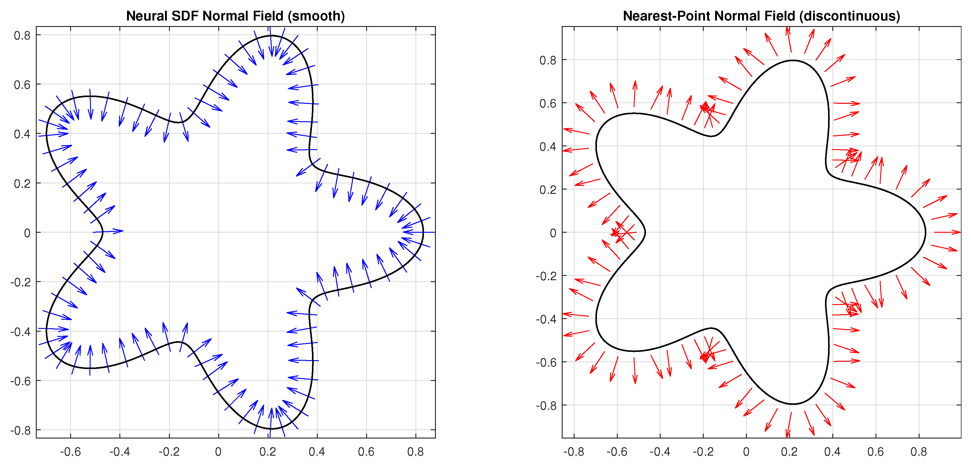
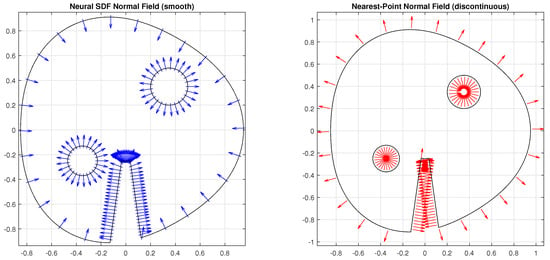
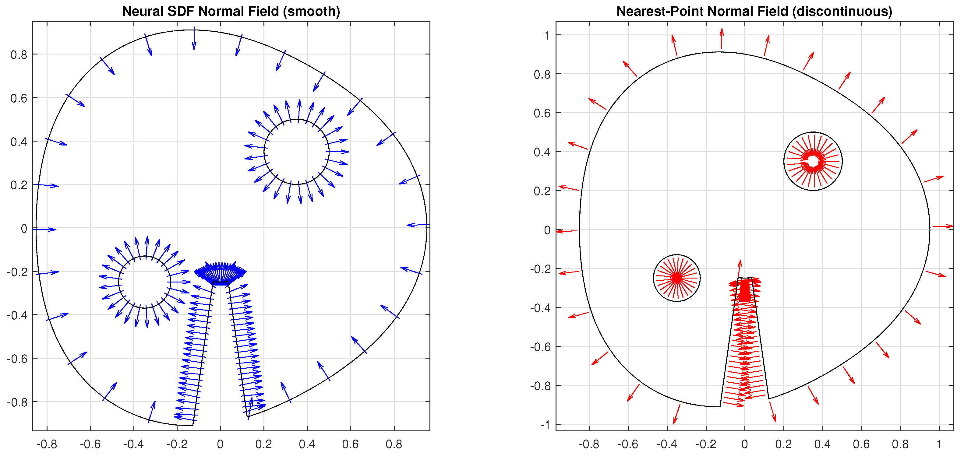
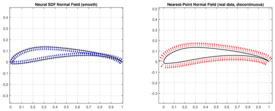
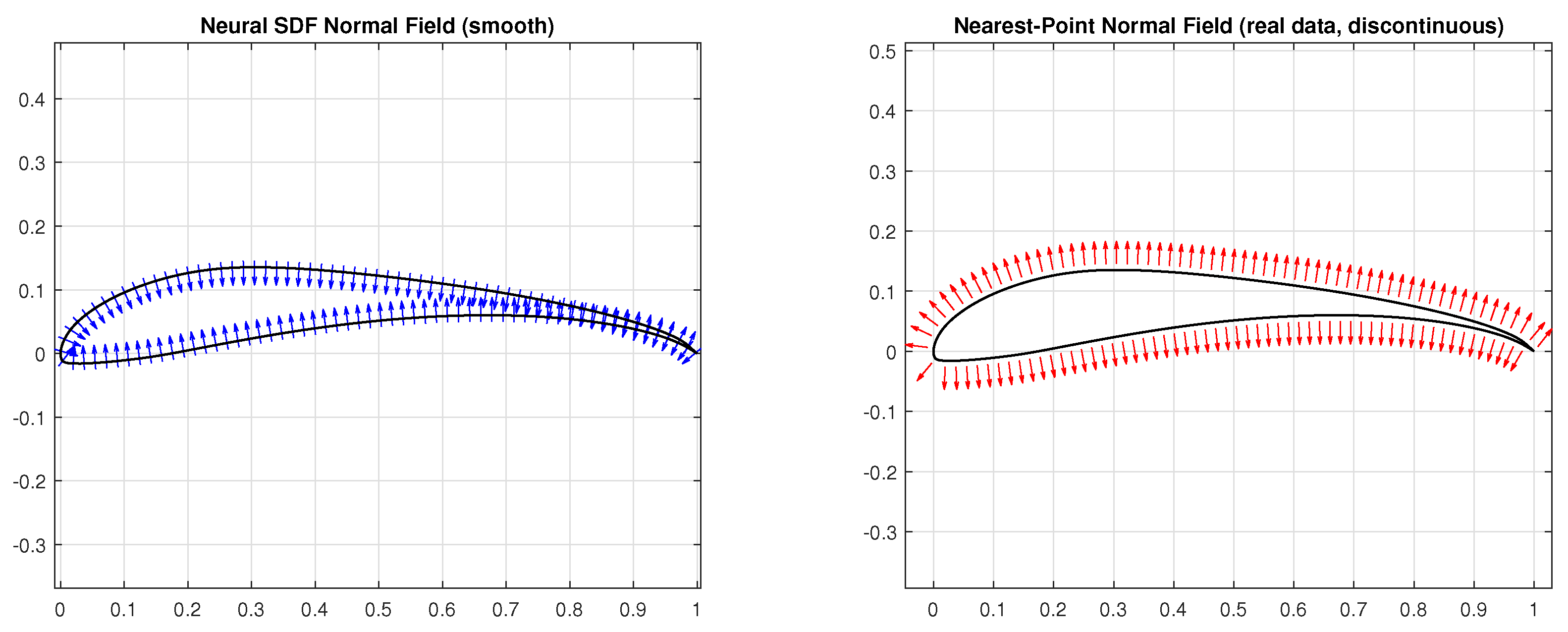
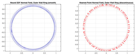
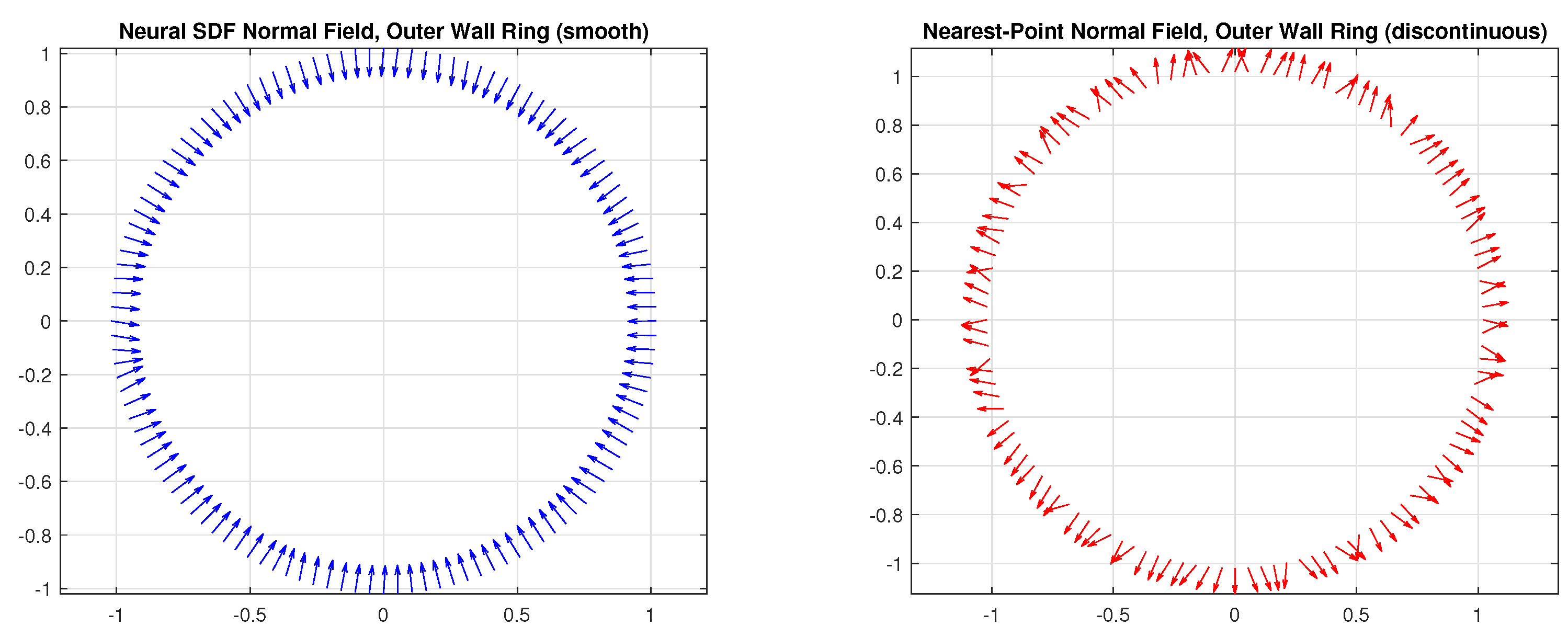
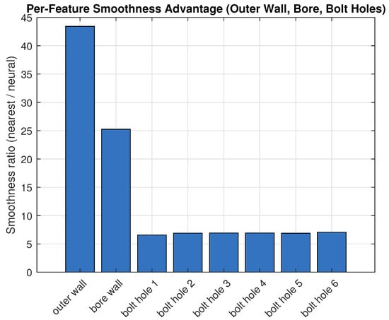
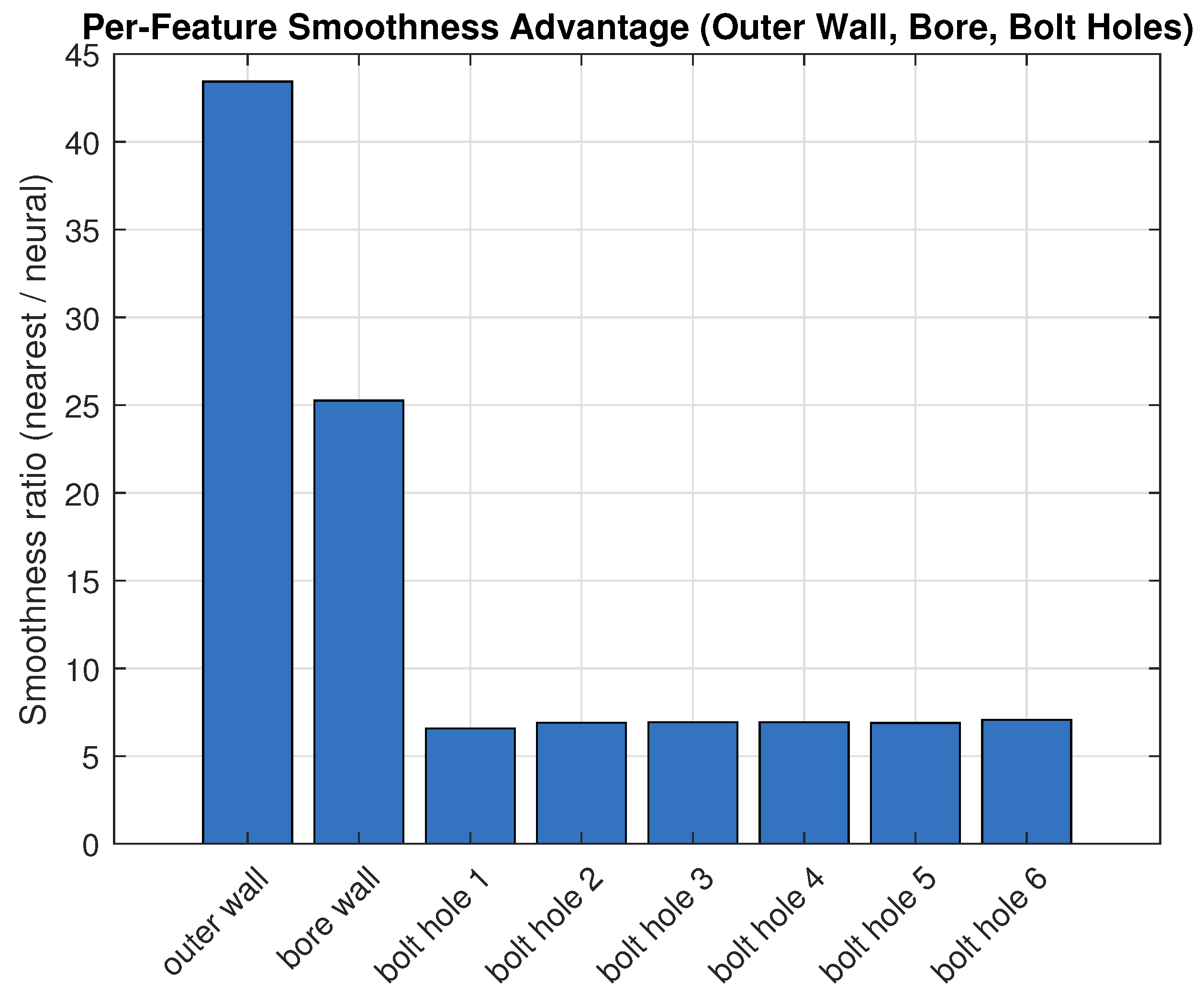

Disclaimer/Publisher’s Note: The statements, opinions and data contained in all publications are solely those of the individual author(s) and contributor(s) and not of MDPI and/or the editor(s). MDPI and/or the editor(s) disclaim responsibility for any injury to people or property resulting from any ideas, methods, instructions or products referred to in the content. |
© 2026 by the authors. Licensee MDPI, Basel, Switzerland. This article is an open access article distributed under the terms and conditions of the Creative Commons Attribution (CC BY) license.