TransformerPIV: An Improved Large-Scale Flow Motion Estimation Method Based on Self-Attention Mechanism

Abstract

Particle image velocimetry (PIV), as a widely used technique for measuring flow velocity fields and characterizing flow behavior, is widely used across various fluid mechanics applications, such as aerodynamics and fluid mechanics. However, the existing PIV methods focus on spatial resolution, i.e., the ability to extract small-scale motions, while ignoring the situation of large-scale flow motion. In this paper, a novel deep learning framework called Transformer is introduced, which is based on the self-attention mechanism and can capture global information. First, in order to enhance the ability to sense location information, convolutional neural network (CNN) is utilized to extract features from original particle images. Second, self-attention mechanism is applied to capture global information based on a set of image features. Third, velocity fields of the particle images are estimated in the encoder-decoder network. Finally, a number of both synthetic and experimental particle images are used to verify the proposed method. The experimental results indicate that the proposed method is superior to cross-correlation and optical flow methods on measurement accuracy. Moreover, it has better performance than traditional deep learning-based PIV methods on large-scale flow motion estimation.

1. Introduction

PIV based on flow visualization not only reveals the physical form of the flow field, but also provides quantitative information of the instantaneous full-field flow, enabling a transition from qualitative to quantitative [1,2,3,4,5,6]. A typical PIV measurement process involves the following steps: the tracer particles are first evenly seeded into the flow field to be measured. Then, a laser beam is reflected by a prism to form a slice of light irradiating the flow field, and the particle images are collected by a CCD camera with successive exposures. Finally, the image processing system analyzes the particle image pairs to obtain the velocity vector distribution of the entire flow field and other quantitative information [7]. This technology has been successfully applied in two-dimensional flow field measurements in both hydrodynamic and aerodynamic experiments, providing an effective means for obtaining detailed velocity distributions and gaining deeper insight into flow structures [8,9]. In addition to conventional planar PIV, three-dimensional PIV techniques, such as stereoscopic and tomographic PIV, have also become well-established tools in experimental fluid mechanics [10,11].

The basic aim of PIV is to extract the corresponding fluid motion velocity field from two consecutive frames of particle images. Traditional PIV processing methods include cross-correlation [12,13,14] and optical flow methods [15,16,17]. The cross-correlation method calculates the mutual correlation by extracting the window of two frames, and it obtains direction by finding the largest correlation function as the displacement vector at the center of that window [18,19]. However, the cross-correlation method calculates the statistical mean displacement within a window, and it is still unable to achieve velocity field estimation with single-pixel level resolution [20,21,22]. As a result, the method cannot satisfy the requirement of small-scale flow motion estimation. Another commonly used PIV method, i.e., the optical flow method, has an advantage in resolution and can calculate the velocity field at the single-pixel level [23,24,25]. However, it is difficult to adjust the hyperparameters of the method. Furthermore, variational optimization in the optical flow method is computationally expensive [26,27].

For the extraction of large-scale coherent structures in complex unsteady flows, post-processing–based modal decomposition methods have been widely applied to the analysis of PIV measurement data [28,29,30], and previous studies have systematically compared the performance of different POD implementations on complex unsteady PIV datasets, providing important guidance for the selection of POD techniques in experimental flow-field post-processing [31]. However, the primary objective of these methods remains focused on the modal decomposition and physical interpretation of already measured flow fields, rather than on directly improving the measurement accuracy of the PIV velocity estimation itself or its capability to cope with large-displacement flows.

In recent years, with the rapid development of artificial intelligence [32], deep learning approaches have been increasingly applied to PIV estimation tasks [26,33,34,35,36]. Rabault et al. [33] demonstrated a proof-of-concept for PIV using artificial neural networks, showing that such models can accelerate and enhance PIV analysis, although their accuracy remains slightly inferior to state-of-the-art cross-correlation methods. Lee [34] developed a convolutional neural network (CNN) framework to improve velocity field estimation and velocity gradient tensor reconstruction, incorporating an outlier detection and replacement strategy. Cai et al. [35] proposed a neural network model capable of generating velocity fields with single-pixel resolution, inspired by PIV-LiteFlowNet-en, an optical flow architecture widely used in computer vision. Zhang et al. [36] introduced an unsupervised optical flow network, UnPWCNet-PIV, which effectively handles particle occlusion and boundary motion, achieving competitive accuracy and robustness on both synthetic and experimental datasets. Despite these advances, existing PIV methods still face challenges in accurately resolving large particle displacements while preserving fine-scale flow structures under practical measurement conditions. Therefore, we apply the Transformer model to the particle image velocimetry to improve the performance of PIV.

In this work, we propose a novel Transformer-based framework for particle image velocimetry (PIV) velocity estimation. The Transformer model, originally introduced by a Google research team [37], is a deep learning architecture based on the self-attention mechanism and was initially developed for natural language processing tasks. Owing to its ability to capture global contextual information and model long-range dependencies, it has recently demonstrated strong performance in various computer vision applications [38,39,40,41,42,43]. The main contribution of this work is the development of a unified PIV velocity estimation framework that integrates convolution-based local feature extraction with attention-based global correlation modeling. Unlike conventional approaches that rely on correlation analysis or incorporate global flow information only in post-processing, the proposed method directly embeds both local particle correspondence and long-range dependencies into the estimation process. This design enables improved accuracy, enhanced robustness, and better preservation of flow structures, particularly in complex flow fields with large particle displacements.

The rest of this paper is organized as follows. Section 2 introduces the overall framework of the proposed Transformer-based deep learning estimator for particle image velocimetry and describes the generation of the synthetic training dataset. Section 3 presents the quantitative evaluations on synthetic flow fields. Section 4 reports the experimental results and comparative analyses on real flow measurements. Section 5 summarizes the main contributions and findings of this study, and Section 6 discusses the limitations of the proposed method and outlines directions for future work.

2. Model Structure

In this section, we introduce the framework of the Transformer for particle image velocimetry and present how to generate the dataset for model training.

2.1. Network Structure and Setting

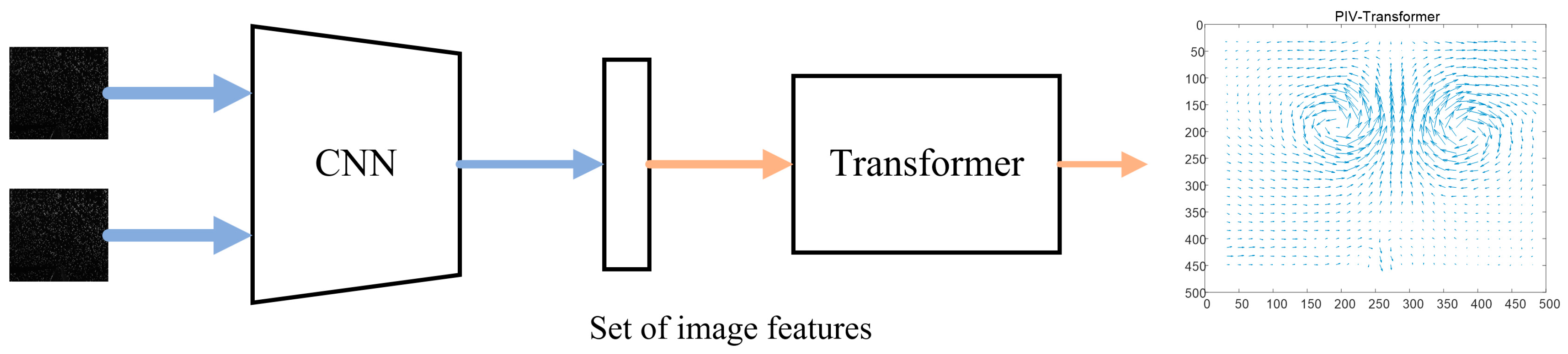
The network structure of the Transformer-based particle image velocimetry method designed in this paper consists of two main components: the CNN backbone network for image features pre-extraction, and the Transformer model for outputting ensemble prediction results (Figure 1).

2.1.1. Encoder and Decoder Stacks

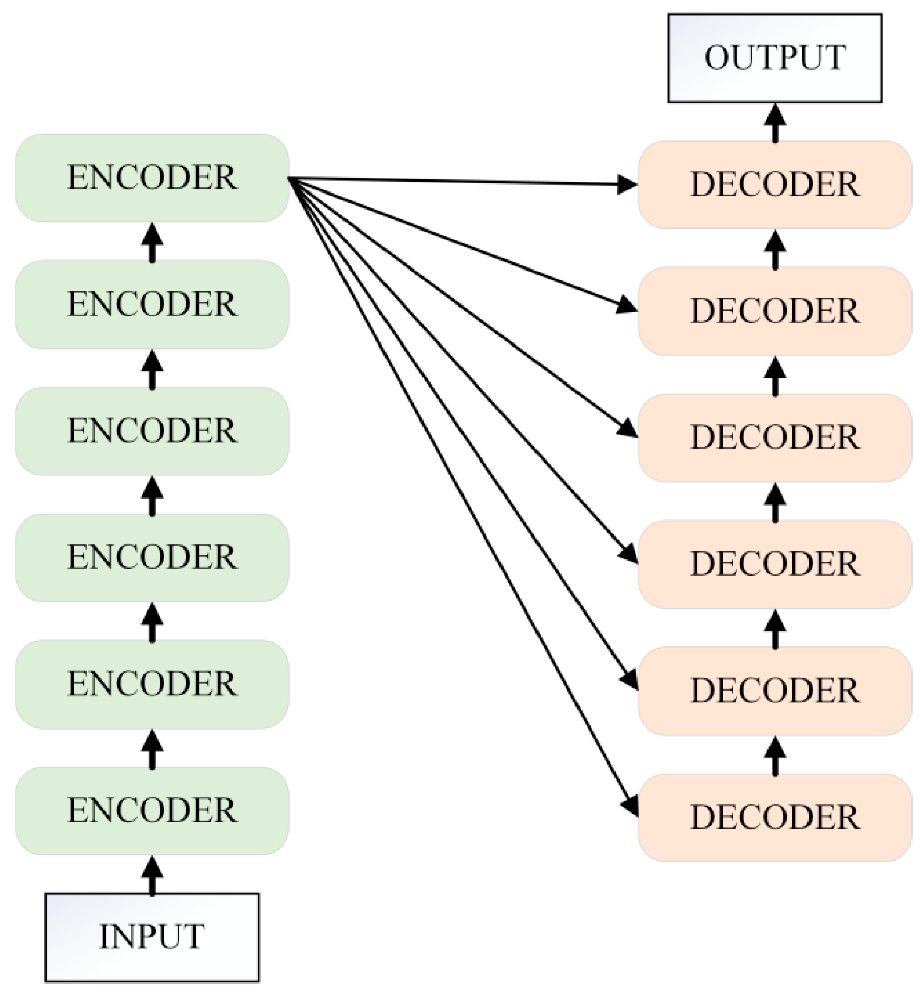
Similar to most sequence models, Transformer is essentially an Encoder-Decoder structure, which constitutes the overall framework of the model by stacking six layers of encoders and decoders (the number of encoders and decoders can be adjusted). This architecture eliminates recurrent connections, which avoids the increase in computational complexity and problems such as gradient vanishing and gradient explosion. As shown in Figure 2, the input of the model passes through all the encoders in order to extract feature representations, and then feeds the processing results into each decoder respectively to get the final output.

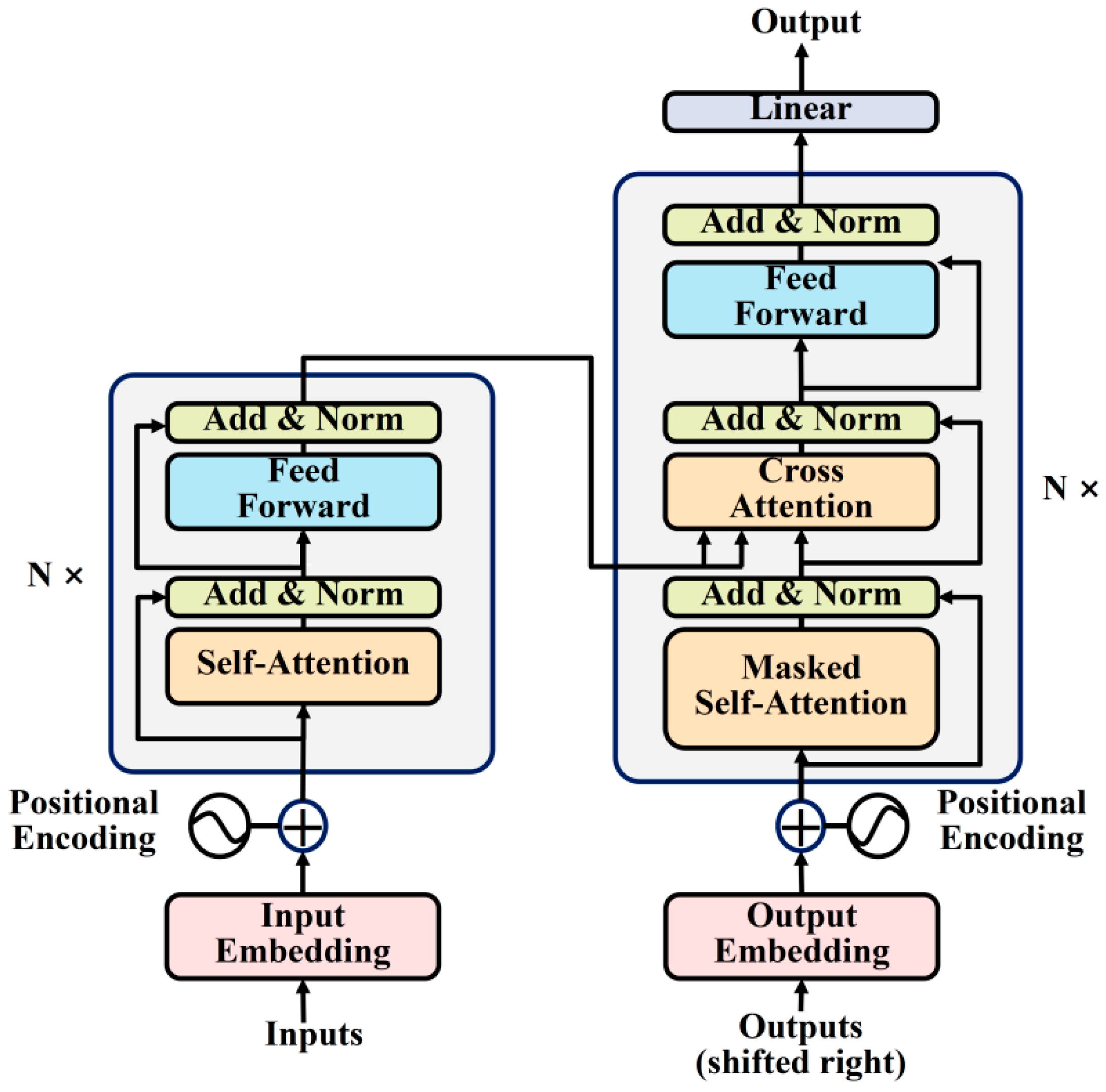
Each of the encoder layers uses the same structure, but they do not have the same parameters and need to be learned separately during the training process. The decoder layers are stacked in the same way. Among them, every encoder layer includes two sub-layers, which are multi-head attention and feed forward; each decoder layer includes three sub-layers, which are masked multi-head attention, multi-head attention, and feed forward. Residual connection is employed around each of the sub-layers, and followed by layer normalization. The overall structure is shown in Figure 3.

2.1.2. Positional Embedding

The input of the Transformer model is different from the traditional cyclic structure such as recursion and convolution. And it inputs all the data into the model in parallel, which lacks the consideration of the relative positional information between the data. Therefore, positional encodings are added to the input embeddings at the bottom of the encoder and decoder stacks. An input vector corresponds to a positional encoding so as to introduce the necessary positional information for each input. What’s more, the positional encodings and the data encoding have the same dimension, so that they can be summed to form the actual input to the model. Positional encodings is performed using the sine-cosine function as shown in the following Equation (1):

$$\begin{array}{l}P{E}_{(pos,2i)}=\sin (pos/{10000}^{2i/d})\\ P{E}_{(pos,2i+1)}=\cos (pos/{10000}^{2i/d})\end{array}$$

(1)

where $pos$ denotes the position of the input data, $i$ denotes the dimension of the position encodings, and each dimension of the position encodings corresponds to a sine-cosine curve. The reason why the sine-cosine function is chosen as the position encodings function is that this function would allow the model to easily learn to attend by relative positions.

Positional encoding effectively addresses the problem of missing relative position information during model input, and the parallel input of the Transformer model greatly improves the computational speed and reduces the storage space compared with the traditional structure.

2.1.3. Feed-Forward Networks

The inputs of the model are passed through a multi-head attention layer into a fully connected feed forward network, which contains two linear transformations with a ReLU activation in between. And the data at each location are processed through this feed forward network separately and identically. Each of the encoder layers and decoders layers uses the same feed forward network, but the parameters are not shared. The complete feed forward network layer can be expressed as follows:

$$FFN(x)=\max (0,x{W}_1+b_1)W_2+b_2$$

(2)

As the encoder and decoder layers are stacked, the depth of the network increases accordingly. To ensure training stability, each sub-layer in both the encoder and decoder is equipped with residual connections and layer normalization. The residual connection adds the input of the preceding layer to its output, which facilitates gradient propagation during backpropagation and alleviates the vanishing gradient problem, thereby improving model performance. Layer normalization operates by normalizing the input across feature dimensions, which stabilizes the learning process and accelerates convergence. The output of each sub-layer can thus be expressed as follows:

$$sub\_layer\_output=LayerNorm(x+SubLayer(x))$$

(3)

2.1.4. Attention Mechanism

The attention mechanism [44] is a key modeling paradigm for sequential data, and its core idea is to assign different weights to different parts of the model, which can be automatically learned and updated by the model. In input sequences, especially long sequences, the attention mechanism allows the model to pay more attention to the parts that are more important for the current output prediction, reducing the time and computational resources of the model to process irrelevant information.

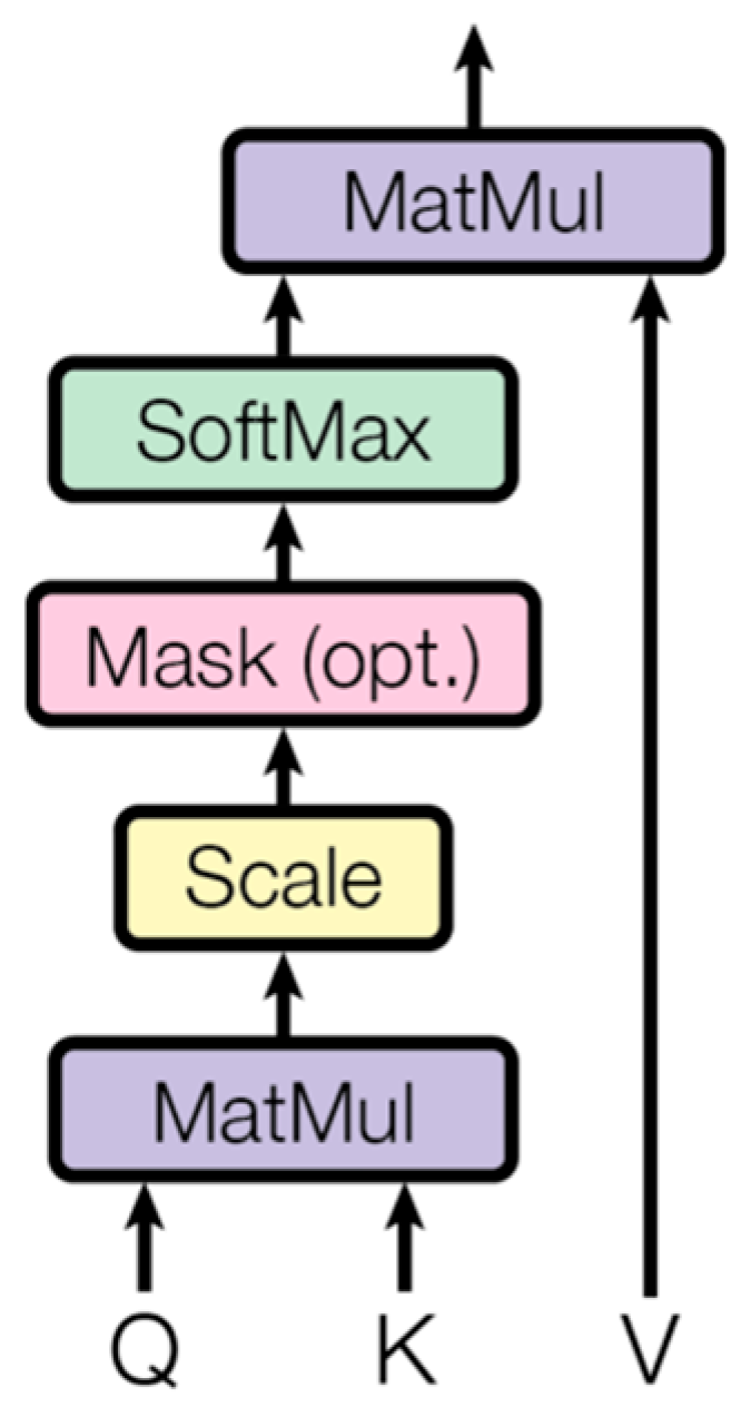
Self-attention mechanism [45] is an improvement of the attention mechanism, which is more adept at capturing correlations within the data or features, and reduces the dependence on external information. Transformer architecture introduces self-attention mechanism that avoids the use of recursion structure in neural networks and relies exclusively on the self-attention mechanism to map the global dependencies between inputs and outputs. The particular attention is called scaled dot-product attention (Figure 4). Compared to general attention, scaled dot-product attention uses dot products for similarity computation, which is faster and more space efficient in practice. The basic structure is shown in Figure 5. The calculation process is shown in the following equation:

$$Attention(Q,K,V)=soft\max ({\displaystyle \frac{Q{K}^T}{\sqrt{d_K}}})V$$

(4)

where $Q,K$, and $V$ matrices represent the Query, Key, and Value, respectively, which are derived by linear transformation of the inputs, and $d_K$ represents the vector dimension.

The steps for calculating the scaled dot-product attention are as follows:

(1)

The inputs of the model are mapped to three different subspaces by linear transformations. Then, we can get the matrices $Q,K$, and $V$ for computation, and the linear transformation matrices are obtained by model training;

(2)

Calculate the dot product of the matrices $Q$ and $K$ to get the attention score, which represents the magnitude of the correlation between the input data at this location and other different locations;

(3)

Divide the obtained attention score by the scaling factor $\sqrt{d_K}$, which makes gradient backpropagation more stable;

(4)

The scaled attention scores are normalized by substituting them into the softmax function, and the attention scores are converted into a probability distribution with a probability sum of 1;

(5)

The matrix $V$ is multiplied with softmax function to expand the difference in attention due to different correlations at different locations;

(6)

Sum the weight vectors to obtain the output of the attention layer at this position.

The above calculation can get the attention scores of the input vectors at a certain position and the input vectors at other positions. The global dependency of the input vectors is obtained by judging the magnitude of their correlation through the attention score.

When processing image data, self-attention layer takes the feature map as input and computes the attention weights between each pair of features to generate an updated feature map where each position has information about any other feature in the same image. These layers can be used directly instead of convolution or in combination with convolutional layers, and they are able to handle a larger sensory field than traditional convolution. Therefore, Transformer is able to capture the dependencies between some long-range spaced features in space.

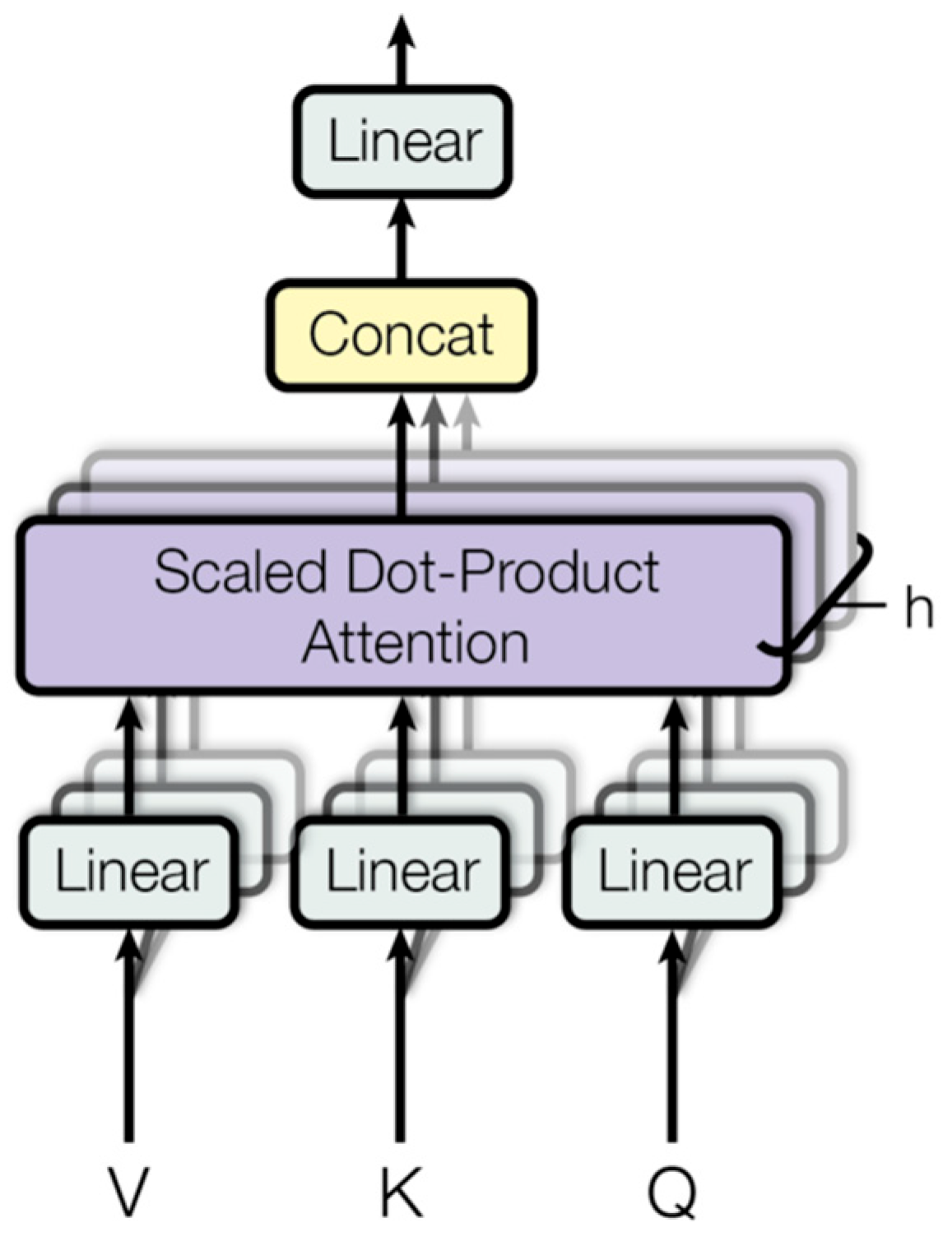
Multi-head attention is a further refinement of the attention layer. Instead of performing a single attention function with $Q,K$, and $V$. Multi-head attention selects several different linear transformation matrices to map $Q,K$, and $V$ to different high-dimensional subspaces, so that the model can pay attention to different parts of the inputs in different subspaces. After a number of parallel computations, the attention information in all subspaces is finally merged. The formula is shown in (5).

$$\begin{array}{c}MultiHead(Q,K,V)=Concat({head}_1,\dots ,{head}_h)W^o\\ {head}_i=Attention(Q{W}_i^Q,K{W}_i^K,V{W}_i^V)\end{array}$$

(5)

where $W^O,W_i^Q,W_i^K,W_i^V$ are linear transformation matrix that can be learned by training.

Since attention is distributed differently in different subspaces, multi-head attention is actually looking for correlations between different perspectives of the input data so that multiple relationships and nuances can be encoded. Its structure is shown in Figure 5. Multi-head attention gives Transformer a powerful structure which allows the model to jointly attend to information from different representation. Thus, more comprehensive and rich features are extracted.

2.1.5. PIV-Transformer

PIV methods need to process the image data to estimate the velocity field, and the information dimension of image data is higher than that of text data. However, the multi-head attention mechanism of the Transformer model will generate a huge computational effort in acquiring global dependencies of the input data, and the computational complexity is quadratic with the resolution of the input image. The two-dimensional images need to be flattened into one-dimensional sequences before they can be fed into Transformer model, and this process does not preserve the relative positional information between the image data. At the same time, subsequent encoder and decoder processing lack the ability to sense location information. These two issues are common to the Transformer model for processing image data.

Convolutional operation makes CNN translation invariant and locally sensitive, so that the relative position information between the input data objects will not be lost in the process of feature extraction. Moreover, it has been demonstrated that the use of Zero Padding in convolutional neural networks preserves the absolute positional information of the input data [46]. Therefore, the input module in Transformer model can be improved by combining CNN, using convolution to obtain local context information, and multi-layer stacking to obtain global relative position relationships. The combination of CNN and Transformer can significantly enhance the location awareness of the model. What’s more, CNN can be regarded as a preprocessing of images, and the features extracted by CNN can be input into the Transformer to reduce the data dimension and the computation of the Transformer model.

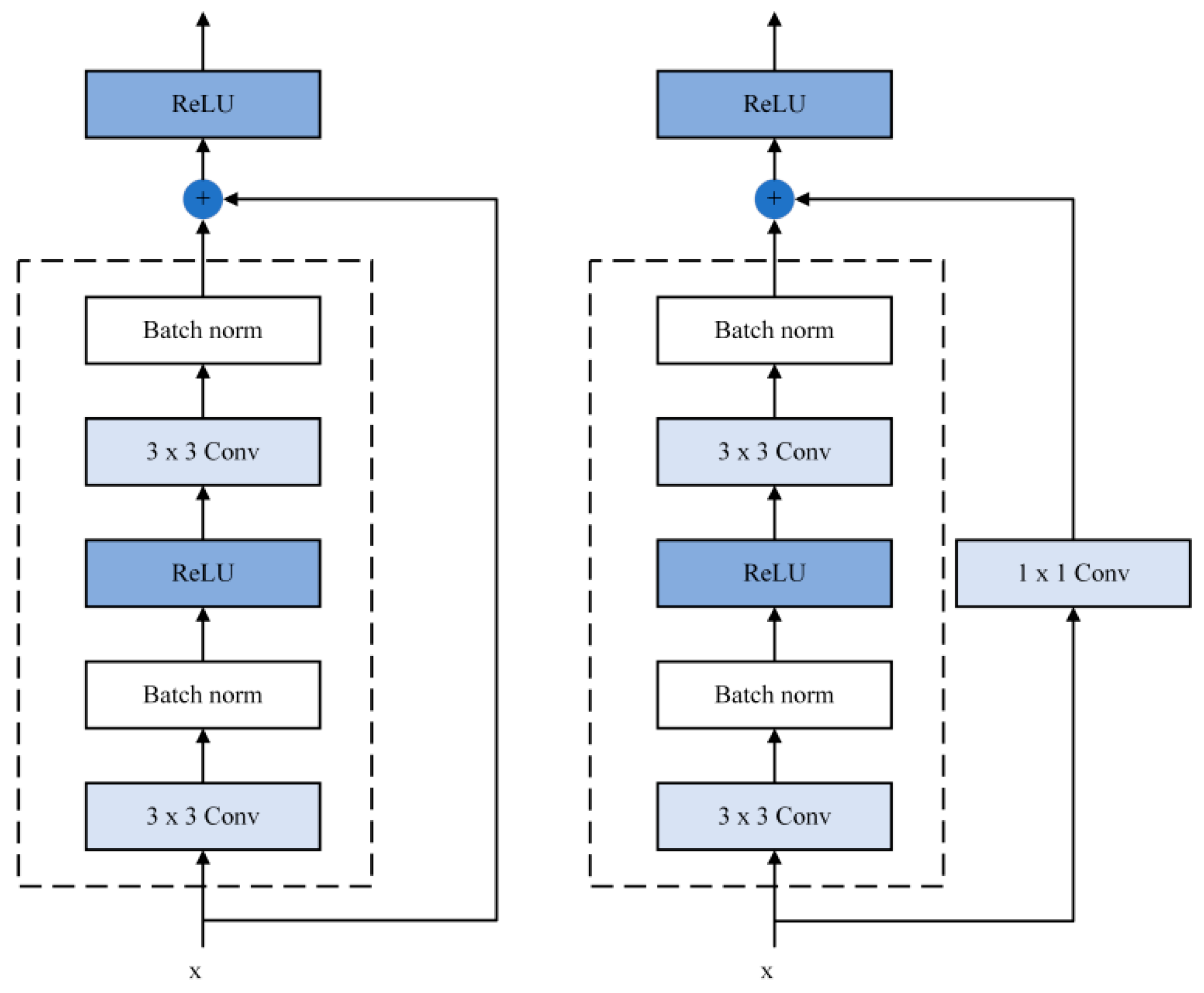
In this paper, we use the first two parts of ResNet18 [47] as the backbone network. The complete ResNet18 network consists of five parts, and each layer of the network has two residual blocks starting with the second part. The residual block structure is shown in Figure 6. The residual structure of the network avoids the problem of gradient vanishing or gradient explosion, thus effectively improving the performance of the model. The number of channels in the residual block can be changed by a 1 × 1 convolution, which ensures that the inputs and outputs have the same channel dimension and can be smoothly summed.

The initial input of the model is $x_{img}\in R^{C_0\times H_0\times W_0}$, where $C_0$ represents the number of particle image pair channels, and $H_0\times W_0$ represents the size of the query window. Since the backbone network uses the first two parts of ResNet18, the input data is downsampled by a factor of 8 to obtain a low-resolution feature map $f\in R^{C\times H\times W}$, where $H,W={\displaystyle \frac{H_0}{8}},{\displaystyle \frac{W_0}{8}}$.

Before inputting the output $f$ of the backbone network to the Transformer encoder, we first use a $1\times 1$ convolution to increase the channels dimension of the map $f$ from $C$ to a higher dimension $d$ to create a new feature map $z_0\in R^{d\times H\times W}$. The encoder requires a one-dimensional sequence as input, so the spatial dimension of $z_0$ needs to be compressed, and the shape of the feature map is transformed to $d\times HW$ At this stage, the feature map is fed into the Transformer encoder, and the encoder output is obtained through positional encoding, multi-head self-attention and feed-forward layers.

The decoder in the proposed network is slightly different from the standard Transformer decoder in that it generates N feature embeddings simultaneously for a given particle image pair, and no masking operation is employed. These embeddings are then projected to velocity vectors through a fully connected regression layer. Here, N denotes the number of output embeddings, and each embedding corresponds to one spatial sampling location in the reconstructed velocity field. Therefore, after the regression layer, N velocity vectors are obtained in one forward pass, and N directly determines the spatial sampling density and hence the spatial resolution of the output velocity field.

2.2. PIV Dataset Generation

The availability and quality of training data play a critical role in neural-network-based PIV, as the performance of the model largely depends on the diversity and quantity of the images used for training. However, the integration of neural networks with PIV is still in its early stages, and existing experimental PIV datasets are insufficient in scale and do not provide pixel-accurate ground-truth displacement fields. For this reason, synthetic datasets are essential: they allow generation of large numbers of particle image pairs with exact ground-truth velocities and enable controlled variation of imaging conditions, such as particle density, noise level, displacement magnitude, and flow deformation. In this study, synthetic data are used to train the model and support systematic evaluation across different flow structures and displacement ranges, while experimental PIV images are employed to further validate the performance and practical applicability of the proposed method under realistic measurement conditions.

Particle Images: Particle image velocimetry technique analyzes the changes of two consecutive frames of particle images to obtain the flow fields information, which is a fundamental requirement for generating simulated particle images. In this paper, we use two methods to generate particle images: the imaging of each particle in the simulated particle motion method is simulated by the point diffusion function, and the motion of the generated particles is simulated by the simulated flow fields; The particle image deformation method needs to refer to the existing particle images, and obtain the relative displacements according to the simulated flow fields. The relative displacements are then applied to the reference image to generate the corresponding particle images, which will be composed of particle image pairs with the original images.

The final step of the simulated particle motion method involves generating particle images from the simulated particle distribution based on an imaging model. In this paper, we use particle image generator [1] which produces artificial particle images with known velocity truth values from manually specified physical simulation parameters. This method is based on the hypothesis that one particle can be described by the 2-D Gaussian function

$$I(x,y)=I_0·\exp \left[-{\displaystyle \frac{{(x-x_0)}^2+{(y-y_0)}^2}{1/8·d_{\tau }^2}}\right]$$

(6)

where the output $I$ denotes the particle brightness at coordinates $(x,y)$ in the image, $I_0$ denotes the peak intensity in the Gaussian center, $(x_0,y_0)$ is the center position of the particle, and $d_r$ denotes the particle imaging diameter. The magnitude of is related to the thickness of the laser sheet.

Flow fields: Both particle image generation algorithms mentioned above are based on simulated flow fields, and in this paper, we use randomly generated simulated flow fields as follows:

$$\begin{array}{cc}\hfill u(x,y)& =P_1+P_{2}y+P_3{y}^2+P_4{y}^3+P_5\sin (P_{6}y+P_7)-P_5\sin (P_7)+P_{15}x+{\displaystyle \frac{1}{2}}{P}_{16}{x}^2+P_{17}xy\hfill \\ & +{\displaystyle \frac{1}{3}}{P}_{18}{x}^3+P_{19}x{y}^2+{\displaystyle \frac{1}{2}}{P}_{20}{x}^{2}y+P_{21}\sin (P_{22}x+P_{23})\cos (P_{24}y+P_{25})-P_{21}\sin (P_{23})\cos (P_{25})\hfill \end{array}$$

(7)

$$\begin{array}{cc}\hfill v(x,y)& =P_8+P_{9}x+P_{10}{x}^2+P_{11}{x}^3+P_{12}\sin (P_{13}x+P_{14})-P_{12}\sin (P_{14})-P_{15}y-P_{16}xy-{\displaystyle \frac{1}{2}}{P}_{17}{y}^2\hfill \\ & -P_{18}{x}^{2}y-P_{19}{y}^3+{\displaystyle \frac{1}{2}}{P}_{20}x{y}^2+P_{21}\cos (P_{22}x+P_{23})\sin (P_{24}y+P_{25})-P_{21}\cos (P_{23})\sin (P_{25})\hfill \end{array}$$

(8)

where u (x, y) and v (x, y) denote the two velocity components of the simulated flow fields at the (x, y) position, $P_1,P_2,\dots P_{25}$ are random data denoting the key parameters constituting the simulated flow fields. It is easy to conclude that when $x=0,y=0$, Equations (7) and (8) can be simplified to $u(x,y)=P_1,v(x,y)=P_8$. Therefore, the velocity vector at the origin of the coordinates of the generated particle image can be controlled by adjusting the parameters $P_1,P_8$. It is also the ground truth needed to construct the dataset.

The synthetic dataset used for training and evaluation consists of particle image pairs generated using the simulated particle motion and image deformation methods. A total of 100 K image pairs are generated, among which 80% are used for training and the remaining 20% are used for testing. It should be emphasized that the proposed network is not trained for any specific flow configuration or flow topology. Before being fed into the network, all particle images are normalized and resized to a fixed resolution. Data augmentation techniques, including translation, rotation, and additive Gaussian noise, are applied during training to improve robustness and generalization. Specifically, translation improves the robustness of the network to spatial misalignment and local displacement variations, rotation enhances the invariance of the model to different flow orientations, and the superimposed Gaussian noise increases robustness against image noise and background contamination. These augmentation operations contribute to more stable training and better generalization under practical PIV imaging conditions.

3. Evaluations on Synthetic Data

In this section, we use image particle generator to generate particle images of the simulated vortex-pair flow field. The vortex-pair flow is selected as a representative benchmark case, because it contains strong velocity gradients and spatially varying displacements, while allowing quantitative error evaluation. Then, our approach is compared with traditional optical flow methods and PIV-DCNN model which is another neural network for PIV estimation.

The performance of the proposed method is evaluated using both quantitative and qualitative metrics. For synthetic datasets with available ground truth, RMSE is used as the primary quantitative metric. For experimental flow data without ground truth, qualitative evaluation is conducted based on velocity field visualization, streamline visualization, and velocity distribution histograms. The RMSE is defined as

$$E_{RMSE}=\sqrt{{\displaystyle \frac{1}{N}}{\displaystyle \sum _{i=1}^N\left[{(u_i^t-u_i^e)}^2+{(v_i^t-v_i^e)}^2\right]}}$$

(9)

where $(u_i^t,v_i^t)$ denote the ground-truth velocity components of the i-th particle, $(u_i^e,v_i^e)$ are the corresponding estimated velocity components, and N is the total number of velocity vectors. As shown in

Table 1. Comparison of RMSE for different PIV methods on the synthetic dataset.

	LK	HS	PIV-DCNN	PIV-Transformer
RMSE	0.039	0.027	0.017	0.015

, the proposed PIV-Transformer yields the smallest RMSE on the synthetic dataset compared with the other methods.

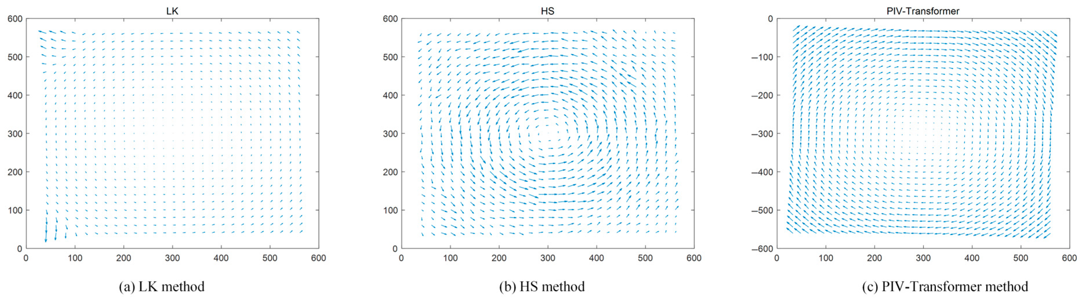
The corresponding velocity-field visualization results obtained by the different methods are shown in Figure 7. The visualization results of both the LK and HS optical flow methods generally reflect the flow direction of the vortex-pair flow field. However, it can also be seen that there is a certain percentage of measurement outliers in the raw results of the LK and HS optical flow methods. And the LK optical flow method has significant deviations in the processing of the upper-left and lower-left corners of the image, which require additional post-processing. Compared to the optical flow methods, the PIV-Transformer method has a higher resolution, exhibits finer structural details and higher measurement accuracy.

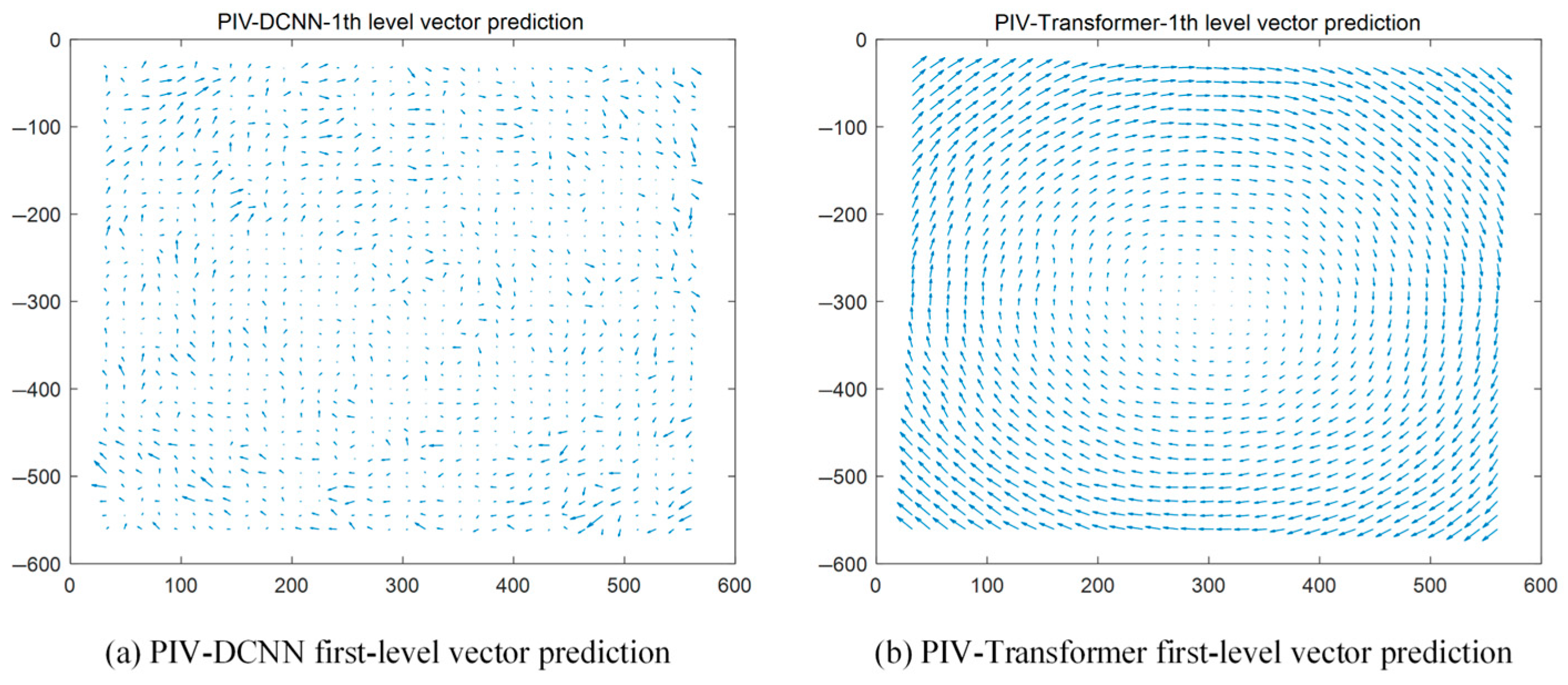
The prediction result of PIV-DCNN model is also satisfactory. But Transformer model single-layer network prediction results do not have significant outliers, the direction of the flow field is clear, and the reliability of the prediction is higher. Take the output of the first-layer network as an example:

From Figure 8 we can see that there are more obvious outliers in the prediction results of PIV-DCNN model, which need to be dealt with the outlier replacement algorithm. However, the outlier replacement algorithm will affect the region where the flow field is correctly predicted at the same time, resulting in the loss of small structure information of the flow field. On the other hand, Transformer model does not need to detect and replace the outliers in the prediction results, which can better preserve the details of the flow field and improve the prediction accuracy.

4. Evaluations on Experimental Data

In order to comprehensively evaluate the model performance, particle images from the PIV particle image library are used for evaluation. And we use standard PIV methods as the comparison methods to compare and analyze with our approach, including the FFTCC method, the WIDIM method [13], and the PIV-DCNN model.

4.1. Test on Vortex Pair Particle Images

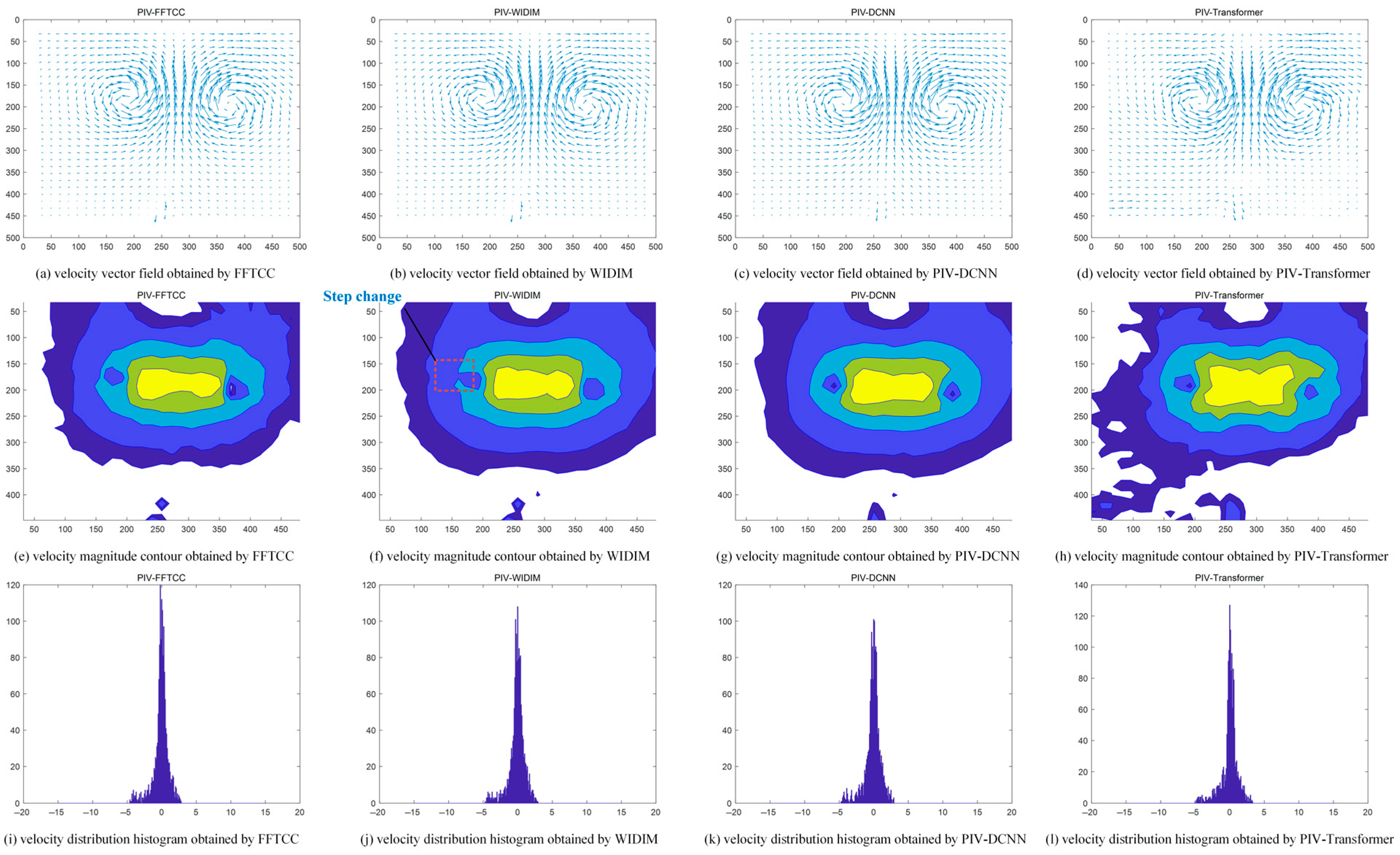
Vortex-pair particle images exhibit little variation in particle diameter, no special particles, moderate particle concentration and uniform distribution, high imaging quality. Although the nozzle position can be observed at the bottom of the image, smooth flow, no flow of very small structures, and a maximum image shift of about 5 pixels, making it well-suited for PIV analysis. The corresponding velocity vector fields, velocity magnitude contours, and velocity distribution histograms are shown in Figure 9.

The measurement results of the four methods are consistent in the visualization, and the difference between the vector field visualization and the velocity distribution histogram is small, which indicates that the prediction results of the four methods are relatively reliable. However, there are some differences in the streamline visualization results. WIDIM method shows an approximate step change, which is different from our theoretical knowledge and belongs to the method error. FFTCC method fails to show the details of the center region of the vortex nucleus very well, and its measurement accuracy is difficult to satisfy the researchers’ needs for the measurements of this flow fields, which is a shortcoming of the method itself.

4.2. Test on Jet Particle Images

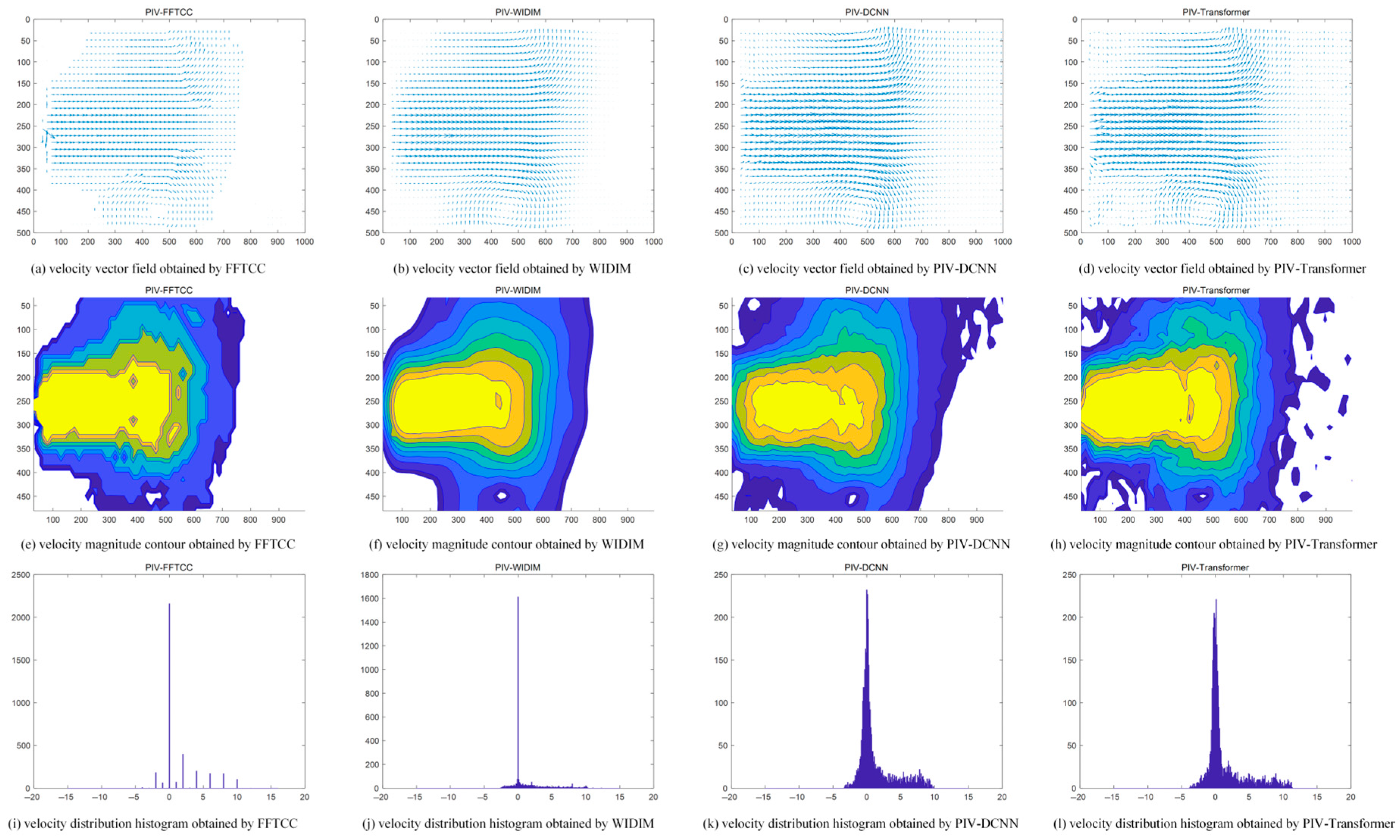
To further evaluate the applicability of the proposed method under practical and challenging experimental conditions, low-quality jet PIV images are also employed. These images exhibit high particle concentration with strongly nonuniform spatial distribution, including regions of clustering and sparseness, together with severe grid-like noise and illumination variation. The particle displacement range is large, reaching nearly 10 pixels near the nozzle and approaching zero farther downstream. In addition, the jet flow itself is highly unsteady, with substantial small-scale fluctuations that further distort particle patterns. These characteristics collectively impose challenges comparable to those encountered in highly turbulent experimental environments, making the jet images a representative and demanding test case for assessing the robustness of the proposed method beyond simplified or canonical flow fields. The corresponding velocity vector fields, velocity magnitude contours, and velocity distribution histograms are shown in Figure 10.

From the vector field visualization, it can be seen that there are certain outliers in the results of FFTCC and WIDIM, and the two methods have absolute zero values in the right region, which is inconsistent with physical observations; From the streamline visualization, it can be seen that the FFTCC method is disturbed by the gridded noise and the measurement results are obviously inconsistent with physical principles. WIDIM method loses the information about the small structure of the flow field, and the prediction result can only roughly reflect the trend of the flow field. PIV-Transformer method preserves more details of the flow field; From the histogram of velocity distribution, it can be seen that FFTCC and WIDIM methods have absolute zero displacement estimation, and FFTCC method has peak locking phenomenon [48]. The histograms of velocity distribution of PIV-DCNN and PIV-Transformer methods are similar. But, PIV-Transformer method has a wider range of velocity measurements and better measures large displacements in the image.

FFTCC and WIDIM are widely recognized as robust and mature PIV techniques, particularly for flows with moderate particle displacements and relatively homogeneous seeding. Although WIDIM improves accuracy through iterative window deformation and multigrid refinement, its performance may degrade in regions with strong velocity gradients and large displacements, and additional post-processing is often required to suppress spurious vectors.

Recent deep-learning-based PIV methods improve robustness and spatial resolution by data-driven feature extraction and end-to-end regression, but most existing PIV-DCNN frameworks rely mainly on convolutional architectures and therefore have limited capability to model long-range particle correlations.

In this study, the proposed Transformer-based method produces velocity fields that are generally consistent with FFTCC, WIDIM and PIV-DCNN, while achieving higher accuracy, improved spatial resolution and fewer outliers, especially in regions with strong displacement gradients and complex flow structures. This improvement is mainly attributed to the self-attention mechanism, which explicitly models global particle correspondences and preserves the spatial coherence of large-scale flow structures without requiring additional post-processing.

5. Conclusions

In this paper, we integrate neural networks with particle image velocimetry and propose a particle image velocimetry method based on Transformer. The PIV particle image dataset is artificially synthesized through the simulated particle motion method and the particle image deformation method, which is used for the supervised learning training of the neural network; finally, we obtain a deep neural network model suitable for the estimation of the fluid motion, achieving higher accuracy compared with the traditional algorithm in the test of the simulated flow field.

In the validation of actual flow field images, the results are compared and analyzed with mainstream methods such as FFTCC and WIDIM through vector field visualization, streamline visualization and velocity distribution histogram. The results demonstrate that the proposed method achieves significantly higher measurement accuracy and spatial resolution than conventional methods, and exhibits improved robustness and reliability under complex flow conditions. This improved performance can be attributed to the ability of the attention mechanism to capture long-range correlations among particle patterns, which helps preserve the spatial coherence of large-scale flow structures, particularly in regions with strong displacement gradients, leading to a more stable and physically consistent reconstruction of the velocity field and a substantial reduction in spurious vectors commonly observed in correlation-based methods. In addition, the proposed Transformer-based PIV approach does not require outlier detection or replacement procedures, thereby avoiding the loss of small-scale flow information and enabling a clearer and more faithful representation of fine flow structures.

These results highlight the methodological contribution of introducing attention-based global correlation modeling into PIV estimation and demonstrate the engineering potential of neural-network-based PIV approaches as a promising data-driven alternative to conventional correlation-based techniques for accurate and reliable flow measurements in complex experimental environments.

6. Limitations and Future Work

Although the proposed Transformer-based PIV method demonstrates improved accuracy and robustness, its current architecture remains computationally more demanding than conventional correlation-based algorithms and typical CNN-based approaches. The relatively large number of model parameters increases memory usage and inference time, which may limit deployment in real-time or resource-constrained measurement systems. In addition, while the method is not tailored to any specific flow topology and is trained on synthetic datasets constructed to cover diverse imaging conditions, its performance may still depend on the breadth and representativeness of the training samples. Expanding the dataset to include more complex and varied flow scenarios will be an important direction for enhancing the generalization capability in future work.

Future work will focus on developing more lightweight network architectures and model compression strategies to reduce computational cost while maintaining or further improving displacement estimation accuracy. In addition, extending the proposed framework to more diverse and complex flow configurations, as well as to three-dimensional PIV measurements, will be investigated to further enhance the general applicability of the proposed method.