Modeling of Biological Neural Networks Based on Neuronal Functions and Connectivity Patterns

Abstract

Despite recent advances in the reconstruction of biological neural networks, the generative principles underlying the structural properties of these networks remain incompletely understood. Neurons in the brain belonging to different functional classes, such as sensory neurons, interneurons, or motor neurons, exhibit distinct connectivity asymmetry patterns. Here, we analyze the differences in connectivity patterns among these types, focusing on the asymmetry between in-degree and out-degree. Our analysis reveals that sensory neurons tend to exhibit a predominance of outgoing connections (negative asymmetry), motor neurons a predominance of incoming connections (positive asymmetry), and interneurons a more balanced connectivity profile. To capture these type-specific features, we propose an extended network growth model in which nodes are assigned to predefined functional types, each with distinct initial attractiveness for incoming and outgoing edges. Simulations demonstrate that our model can reproduce the observed asymmetry indices of different neuron types in biological neural networks and can also generate diverse degree distribution shapes. This work offers a phenomenological generative framework that links neuron type identity to connectivity asymmetry, and it provides a baseline for future studies that incorporate additional biological constraints.

1. Introduction

Biological neural networks encompass neurons and connections, which are analogous to the nodes and edges of artificial neural networks. Neurons are the most fundamental structural and functional units of the biological nervous system, and they can be classified based on morphology, neurotransmitter type, or function [1,2,3]. From functional and connectomic perspectives, a particularly relevant classification divides neurons into three broad categories, that is, sensory neurons (afferent), motor neurons (efferent), and interneurons. Sensory neurons receive external signals and transmit them inward, motor neurons send commands to muscles, and interneurons mediate local and global communication between them. This tripartite classification provides a fundamental framework for analyzing circuit structure in many reconstructed connectomes at single-neuron resolution [4,5,6].

To date, synapse-resolution connectomes have been reconstructed for the nematode C. elegans [4,5,6,7], the central nervous system of a tadpole larva of Ciona intestinalis (L.) [8], the larval and adult Drosophila [9,10,11,12,13,14,15,16,17,18], the inner plexiform layer in the mouse retina [19], and so on. Network analysis of these connectomes has revealed non-random structural properties including small-world properties [20,21,22,23], network motifs [14,18,23,24,25], modules and rich clubs [6,7,18,23,26], and characteristic degree distributions [23]. While these empirical patterns are robust across species, a generative framework that links neuron type identity to emergent circuit structure is still lacking.

A variety of network growth models have been proposed to explain the emergence of structural properties in complex networks. Classical models based on preferential attachment, initial attractiveness, fitness, aging, and cost have successfully reproduced scale-free and other properties observed in social, citation, and biological networks [27,28,29,30,31,32,33,34,35,36,37]. For the C. elegans neural network, several models have been proposed. For instance, a distance-dependent model [20] and two gene-expression-based models [38,39] captured specific features of the C. elegans connectome, such as spatial clustering or the formation of gap junctions. More recently, our previous work developed a growth model that incorporates distinct initial attractiveness for in-degrees and out-degrees, combined with preferential attachment [40]. This model successfully reproduced the global asymmetry between incoming and outgoing connections observed in developmental C. elegans connectomes, as well as the overall shape of the degree distributions.

In spite of these advances, a significant gap remains in existing models: they treat all neurons as a single homogeneous population. Empirical observations in C. elegans and other connectomes reveal substantial differences in connectivity patterns across functional neuron types. Specifically, sensory neurons tend to exhibit a predominance of outgoing connections (negative asymmetry), motor neurons exhibit a predominance of incoming connections (positive asymmetry), and interneurons display a more balanced profile. Because prior models do not distinguish between neuron classes, they are inherently unable to reproduce this observed variance in type-specific asymmetry indices.

To fill this gap, we propose an extended network growth model, in which nodes are assigned to distinct functional types—sensory neurons, interneurons, and motor neurons, and each type is governed by type-specific initial attractiveness parameters for in-degree and out-degree. In this study, we first analyze the asymmetry indices and the in-degree versus out-degree distributions across these three neuron classes in developmental C. elegans connectomes and other neuronal networks. We then formalize the extended model and systematically investigate how variations in the type-specific parameters shape the emergent degree distributions and asymmetry profiles. This work provides a phenomenological generative model that reproduces class-specific degree asymmetry, serving as a baseline for future models incorporating additional biological constraints.

2. Materials and Methods

2.1. Biological Neural Networks

The developmental C. elegans connectomes analyzed in this study are provided by [6]. Among the eight datasets, four are from the first larval stage (L1, from hatching to the first molt), one from the second larval stage (L2, from the first molt to the second molt), one from the third larval stage (L3, from the second molt to the third molt), and the remaining two are from the adult stage (Adult). The fourth larval stage (L4) spans from the third molt to the fourth molt. After experiencing the fourth molt, C. elegans becomes a mature adult. Additional connectomes analyzed in this work include the C. elegans hermaphrodite and male connectomes [5], the Drosophila larval visual system [9], the left Drosophila larval olfactory system [10], the Drosophila larval mushroom body (MB) [11], the Drosophila optic medulla [13], the Ciona intestinalis CNS [8], and the mouse retinal inner plexiform layer (IPL) [19]. The adult Drosophila central brain connectome (referred to as the hemibrain, v1.1 release) was downloaded from https://www.janelia.org/project-team/flyem/hemibrain (accessed on 27 July 2020). Except for the adult Drosophila hemibrain, neurons in all other neuronal networks have been functionally identified as sensory neurons, interneurons or motor neurons. We only analyze the directed chemical networks composed of neurons and connections formed by chemical synapses. The number of different types of neurons in these biological neural networks is shown in

Table 1. The asymmetry index between in-degree and out-degree of different types of neurons in C. elegans connectomes across development. N: the total number of neurons in the dataset; E: the total number of chemical connections between neurons in the dataset; $N_S$: the number of sensory neurons in the dataset; ${\alpha }_S$: the asymmetry index of sensory neurons; $N_I$: the number of interneurons in the dataset; ${\alpha }_I$: the asymmetry index of interneurons; $N_M$: the number of motor neurons in the dataset; ${\alpha }_M$: the asymmetry index of motor neurons.

Stages	L1				L2	L3	Adult
Dataset	1	2	3	4	5	6	7	8
N	161	162	162	168	173	174	180	180
E	675	865	887	1011	1324	1314	1933	1933
C	0.126	0.141	0.154	0.152	0.164	0.169	0.183	0.189
L	2.989	2.801	2.823	2.816	2.964	2.794	2.545	2.508
$\alpha$	−0.080	−0.054	−0.059	−0.016	0.003	−0.005	0.017	0.016
$N_S$	57	57	57	61	63	63	65	65
${\alpha }_S$	−0.326	−0.280	−0.329	−0.226	−0.261	−0.303	−0.253	−0.250
$N_I$	66	67	67	67	69	69	73	73
${\alpha }_I$	−0.015	−0.054	−0.042	−0.052	−0.003	−0.001	−0.009	0.001
$N_M$	38	38	38	40	41	42	42	42
${\alpha }_M$	0.176	0.287	0.318	0.366	0.419	0.436	0.479	0.456

and

Table 2. The asymmetry index between in-degree and out-degree of different types of neurons in other biological neural networks.

Neuronal Network	C	L	$\mathit{\alpha }$	${\mathit{N}}_{\mathit{S}}$	${\mathit{\alpha }}_{\mathit{S}}$	${\mathit{N}}_{\mathit{I}}$	${\mathit{\alpha }}_{\mathit{I}}$	${\mathit{N}}_{\mathit{M}}$	${\mathit{\alpha }}_{\mathit{M}}$
C. elegans herm	0.245	2.816	0.008	83	−0.251	91	−0.059	126	0.227
C. elegans male	0.139	2.674	0.021	137	−0.202	123	0.007	118	0.293
Drosophila larval visual system	0.354	1.015	−0.252	29	−0.930	29	0.426
Drosophila larval olfactory system (left)	0.463	1.743	0.065	21	−0.507	75	0.225
Drosophila larval MB	0.424	2.089	−0.001			309	−0.001
Drosophila optic medulla	0.139	2.674	0.067			343	0.067
The adult Drosophila hemibrain			−0.019
Ciona CNS	0.359	2.296	−0.004	37	−0.114	125	0.004	14	0.223

.

2.2. Asymmetry Analysis

The asymmetry of a network quantifies the tendency of nodes to have unbalanced out-degree and in-degree. To capture both the magnitude and directionality of this imbalance, we adopt the modified asymmetry index ${\alpha }_i$ for node i proposed in [40]:

$${\alpha }_i={\displaystyle \frac{k_i^{in}-k_i^{out}}{k_i^{in}+k_i^{out}}}.$$

(1)

Here, ${\alpha }_i>0$ indicates a predominance of incoming connections, ${\alpha }_i<0$ indicates a predominance of outgoing connections, and ${\alpha }_i=0$ indicates balanced in-degree and out-degree. The average value of the ${\alpha }_i$’s throughout the network, $\alpha$, is computed as follows:

$$\alpha ={\displaystyle \frac{1}{N}}{\sum }_{i=1}^N{\alpha }_i.$$

(2)

where N is the total number of nodes in the network.

In the biological neural networks studied here, neurons are grouped into sets of sensory neurons (S), interneurons (I), and motor neurons (M). The average asymmetry index for each neuron class is calculated as follows:

$${\alpha }_C={\displaystyle \frac{1}{N_C}}{\sum }_{i\in C}{\alpha }_i,C\in \{S,I,M\},$$

(3)

where $N_C$ is the number of neurons in class C.

2.3. Degree Distribution

The probability density function $p\left(k\right)$ of the degree distribution is defined as the fraction of nodes in the network with degree k:

$$p\left(k\right)={\displaystyle \frac{N\left(k\right)}{N}},$$

(4)

where $N\left(k\right)$ is the number of nodes with degree k. In directed networks, k refers to either the in-degree $k^{\mathrm{in}}$ or the out-degree $k^{\mathrm{out}}$, and their distributions are analyzed separately.

2.4. Clustering Coefficient and Path Length

The average clustering coefficient and the average shortest path length are two key characteristics that quantify small-world properties. The local clustering coefficient $c_i$ of node i is defined as the fraction of triangles that actually exist over all possible triangles in its neighborhood, defined by

$$C_i={\displaystyle \frac{2E_i}{k_i(k_i-1)}},$$

(5)

where $E_i$ is the number of edges among the $k_i$ neighbors of node i, excluding edges between the neighbors and node i itself. The average clustering coefficient C of the network is

$$C={\displaystyle \frac{1}{N}}{\sum }_i^N{C}_i.$$

(6)

The shortest path length $d_{ij}$ between node i and node j is defined as the minimum number of edges that must be traversed from i to j, and the average shortest path length L of a network is

$$L={\displaystyle \frac{1}{N(N-1)}}\sum _{i\ne j}{d}_{ij},$$

(7)

A network is considered to exhibit small-world properties if it has a significantly higher C and a comparable L relative to a random network.

2.5. Network Growth Model and Simulation

The extended network growth model is described in detail in Section 3.2. All simulations were performed in Python 3.7 using the NetworkX library. For each parameter set investigated, we generated $n=100$ independent realizations of the network growth process.

3. Results

3.1. Differences in Asymmetry of Different Types of Neurons in Biological Neural Networks

In the reconstructed biological neural networks analyzed here, neurons have been functionally classified as sensory neurons, interneurons, or motor neurons based on their function, location, and morphology. The modified asymmetry index defined in Equation (1) captures both the magnitude and direction of degree imbalance. While prior work has shown that the global asymmetry index of the C. elegans connectome increases across development and remains overall positive [40], the distribution of asymmetry across functional neuron types has not yet been quantified.

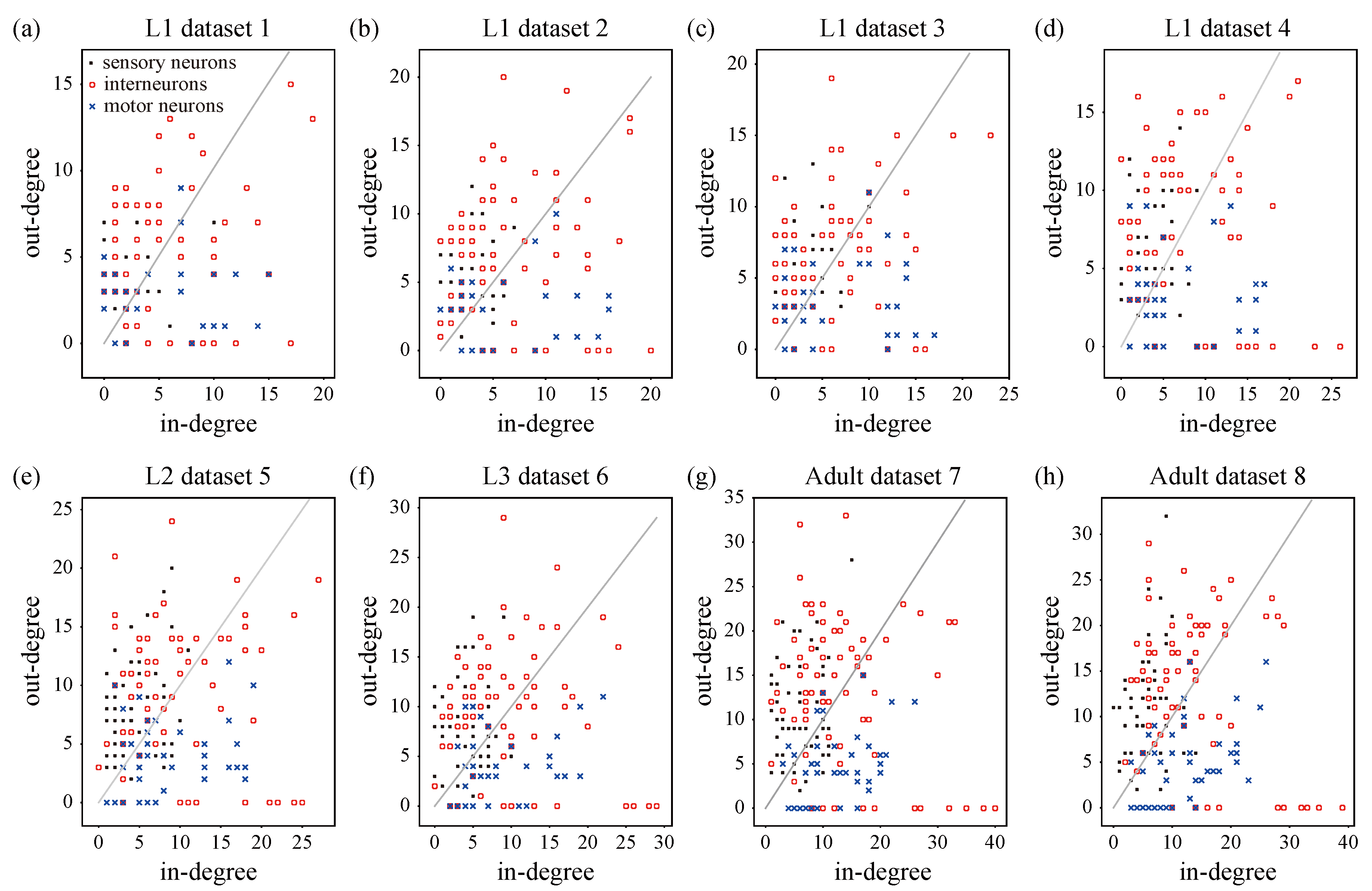
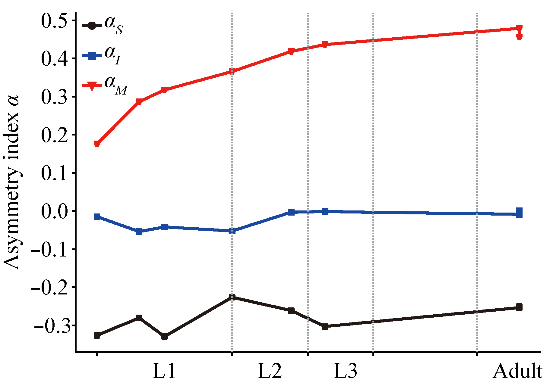
To this end, we plotted the in-degree versus out-degree distributions for each neuron type across developmental stages of C. elegans (Figure 1) and computed the corresponding asymmetry indices ${\alpha }_S$, ${\alpha }_I$, and ${\alpha }_M$ (Table 1 and Figure 2). As shown in Figure 1, sensory neurons predominantly lie above the diagonal (indicating $k^{\mathrm{out}}>k^{\mathrm{in}}$), motor neurons lie predominantly below the diagonal ($k^{\mathrm{in}}>k^{\mathrm{out}}$), and interneurons span a broad range with many exhibiting high total degree. Quantitatively, in the developmental C. elegans connectomes, ${\alpha }_S$ ranges from $-0.329$ to $-0.226$, ${\alpha }_M$ increases with age from $0.176$ to approximately $0.468$ (averaged across the two adult replicates), and ${\alpha }_I$ remains relatively stable near zero (Table 1).

We further quantified asymmetry indices in other biological neural networks (Table 2). In the C. elegans hermaphrodite, male, and Ciona CNS connectomes, ${\alpha }_S$ is $-0.251$, $-0.202$, and $-0.114$, respectively. ${\alpha }_I$ is $-0.059$, $0.007$, and $0.004$, respectively. ${\alpha }_M$ is $0.227$, $0.293$, and $0.223$, respectively. In the neural networks of the Drosophila larval visual system and the left Drosophila larval olfactory system, neurons are classified into sensory neurons and interneurons according to the location and function of the reconstructed area. In the Drosophila larval visual system, $\alpha$ is $-0.252$, ${\alpha }_S$ is $-0.930$, and ${\alpha }_I$ is $0.426$. In the left Drosophila larval olfactory system, $\alpha$ is $0.065$, ${\alpha }_S$ is $-0.507$, and ${\alpha }_I$ is $0.225$. In the neural networks of the Drosophila larval mushroom body (MB) and the Drosophila optic medulla, all neurons are interneurons, and the overall asymmetry index $\alpha$ is $-0.001$ and $0.067$, respectively. For the adult Drosophila hemibrain, neurons were not classified into the three types, and the overall asymmetry index $\alpha$ is $-0.019$. Therefore, in biological neural networks containing multiple neuron types, different neuron types show obvious differences in their in-degree and out-degree asymmetry indices, which are closely related to the functional characteristics of the different neuron types.

Taken together, these results quantitatively confirm that the direction and magnitude of degree asymmetry are closely aligned with neuronal function. Sensory neurons predominantly send synaptic outputs to downstream neurons, motor neurons predominantly receive synaptic inputs from upstream neurons, and interneurons exhibit relatively balanced connectivity with both afferent and efferent populations.

3.2. The Extended Model

In the biological neural networks analyzed above, the asymmetry index differs across functional neuron types. When a connectome contains all three types, sensory neurons exhibit negative asymmetry indices (${\alpha }_S<0$), motor neurons exhibit positive asymmetry indices (${\alpha }_M>0$), and interneurons show intermediate values near zero. The network growth model proposed in [40] introduced distinct initial attractiveness for in-degrees and out-degrees, and it successfully reproduced the global asymmetry and degree distribution shapes of developmental C. elegans connectomes. However, this model treats all nodes as a homogeneous population, which cannot capture the observed type-specific differences in asymmetry indices across sensory neurons, interneurons, and motor neurons. Here, we propose an extended model in which nodes are partitioned into three functional types, each governed by type-specific initial attractiveness parameters for in-degrees and out-degrees.

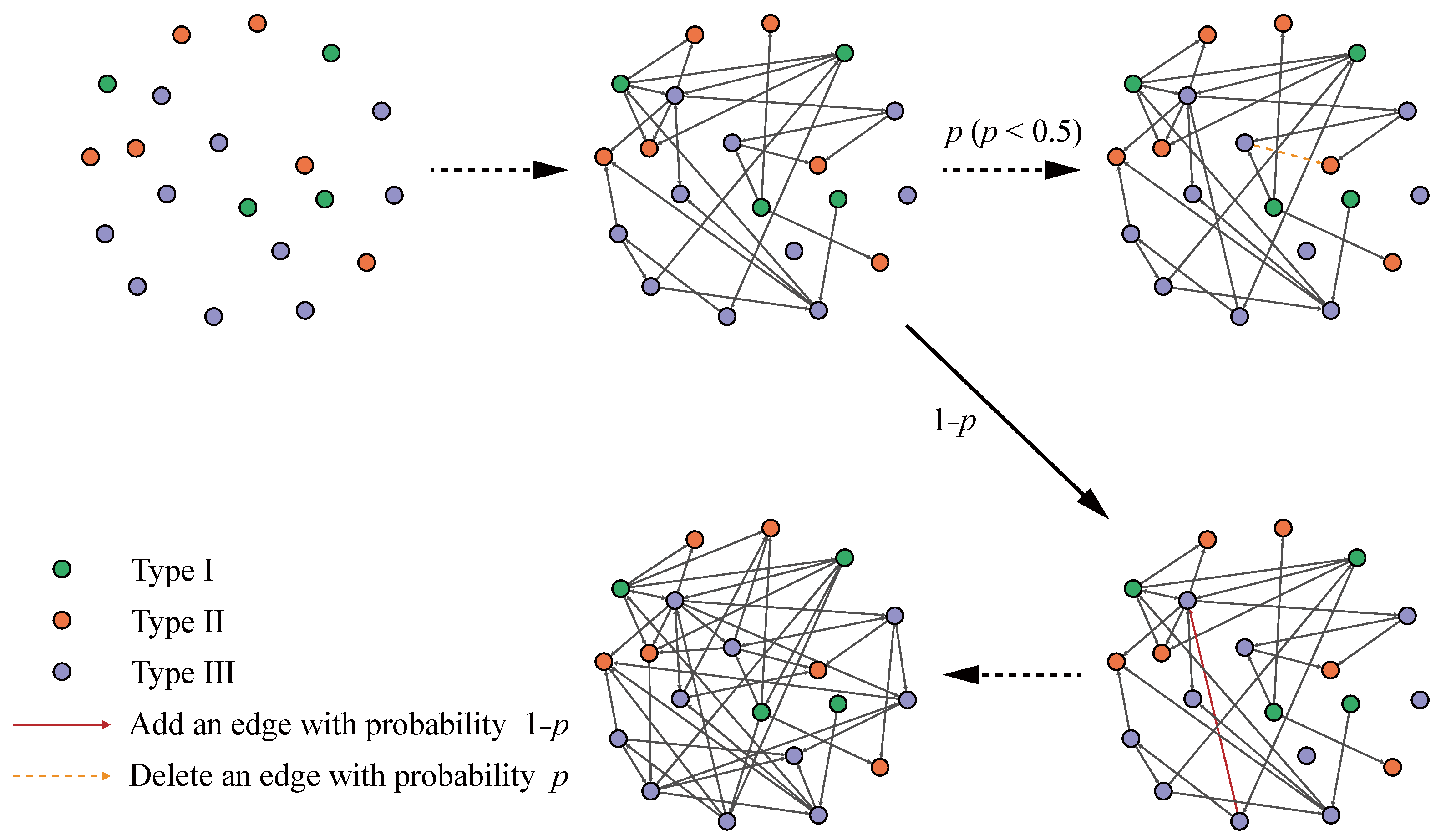
The extended model begins with N isolated nodes. As illustrated in Figure 3, the N nodes are partitioned into three types, namely, type I, type II, and type III, corresponding, respectively, to sensory neurons, interneurons, and motor neurons in biological neural networks. The proportions of type I, type II, and type III nodes are controlled by parameters $s_r$ and $m_r$, where $s_r=N_S/N$ and $m_r=N_M/N$ denote the fractions of sensory and motor neurons, respectively. The initial attractiveness for in-degrees and out-degrees is specified by type-specific parameters, $(a_{\mathrm{in}},a_{\mathrm{out}})$ for type I (sensory neurons), $(b_{\mathrm{in}},b_{\mathrm{out}})$ for type II (interneurons), and $(c_{\mathrm{in}},c_{\mathrm{out}})$ for type III (motor neurons). These parameters are nonnegative integers. Biologically, the type-specific initial attractiveness parameters can capture the propensity of a neuron to establish incoming or outgoing connections. For sensory neurons, which act as signal senders, $a_{\mathrm{in}}<a_{\mathrm{out}}$ indicates an intrinsic bias toward extending outgoing projections (e.g., axons) to interneurons or motor neurons, rather than receiving inputs. Conversely, for motor neurons, which act as command recipients, $c_{\mathrm{in}}>c_{\mathrm{out}}$ reflects their inherent preference for forming incoming connections. For interneurons, which serve as relays, $b_{\mathrm{in}}\approx b_{\mathrm{out}}$, and it maintains relatively equal in- and out-degree propensities. These parameters can be interpreted as simplified proxies for genetic or molecular determinants of synaptic connectivity, such as cell-adhesion molecules or axon guidance cues, which are known to bias connection formation in a type-specific manner. Therefore, we impose the following constraints: $a_{\mathrm{in}}<a_{\mathrm{out}}$, $c_{\mathrm{in}}>c_{\mathrm{out}}$, and $b_{\mathrm{in}}\approx b_{\mathrm{out}}$. Additional relative constraints (e.g., $a_{\mathrm{in}}<b_{\mathrm{in}},c_{\mathrm{in}}$ and $a_{\mathrm{out}},c_{\mathrm{out}}<b_{\mathrm{out}}$) reflect the general tendency for interneurons to have higher overall degrees than sensory and motor neurons.

At each time step, one of the following two operations is performed (see Figure 3).

(1)

With probability $p(p<0.5)$, we randomly remove an existing directed edge from the network, provided that the network contains at least one edge. This mimics biological processes such as synaptic pruning and activity-dependent refinement during neural development.

(2)

With probability $1-p$, we add a new directed edge. The source node i and target node j are selected independently, with probabilities proportional to their respective out-degree, in-degree, and initial attractiveness. Let $A_u^{\mathrm{out}}$ and $A_u^{\mathrm{in}}$ denote the initial attractiveness parameters for out-degree and in-degree of node u, respectively, where the specific values of these parameters depend on the node type:

$$(A_u^{\mathrm{out}},A_u^{\mathrm{in}})=\left\{\begin{array}{cc}(a_{\mathrm{out}},a_{\mathrm{in}}),\hfill & \mathrm{if}u\in \mathrm{Type}\mathrm{I}(\mathrm{sensory}\mathrm{neurons}),\hfill \\ (b_{\mathrm{out}},b_{\mathrm{in}}),\hfill & \mathrm{if}u\in \mathrm{Type}\mathrm{II}\left(\mathrm{interneurons}\right),\hfill \\ (c_{\mathrm{out}},c_{\mathrm{in}}),\hfill & \mathrm{if}u\in \mathrm{Type}\mathrm{III}(\mathrm{motor}\mathrm{neurons}).\hfill \end{array}\right.$$

The probability of selecting node i as the source of the new edge is then

$${\Pi }_i^{\mathrm{out}}={\displaystyle \frac{k_i^{\mathrm{out}}+A_i^{\mathrm{out}}}{{\sum }_{u=1}^N\left(k_u^{\mathrm{out}}+A_u^{\mathrm{out}}\right)}},$$

(8)

and the probability of selecting node j as the target is

$${\Pi }_j^{\mathrm{in}}={\displaystyle \frac{k_j^{\mathrm{in}}+A_j^{\mathrm{in}}}{{\sum }_{u=1}^N\left(k_u^{\mathrm{in}}+A_u^{\mathrm{in}}\right)}}.$$

(9)

The new edge $e_{ij}$ is then added from i to j.

According to the model rules defined above, nodes of different types have distinct probabilities of being selected as the source or target of a new edge. Specifically, type I (sensory) nodes have a lower probability of gaining the out-degree compared to type II and type III nodes, whereas type III (motor) nodes have a lower probability of gaining the out-degree compared to type I and type II nodes. Consequently, the extended model generates networks in which the asymmetry indices differ across node types, which is consistent with empirical observations.

To understand how the degree of a node evolves over time as a function of its type, we analyze the continuous-time rate equations for the growth dynamics. For brevity, we present the derivation for in-degree; the out-degree dynamics follow an entirely analogous procedure with “in” replaced by “out” and the corresponding type-specific attractiveness parameters.

Let $k_i^{\mathrm{in}}\left(t\right)$ denote the in-degree of node i at time t, and assume the node belongs to a generic type $T\in \{\mathrm{I},\mathrm{II},\mathrm{III}\}$ with corresponding in-degree initial attractiveness $A_T^{\mathrm{in}}$. The rate of change of $k_i^{\mathrm{in}}$ comprises two processes:

(1)

Edge removal: With probability p, a randomly selected existing edge is removed. The probability that node i loses an in-degree is proportional to $1/E\left(t\right)$, where $E\left(t\right)=(1-2p)t$ is the number of edges at time t. Thus,

$${\left.{\displaystyle \frac{\partial k_i^{\mathrm{in}}}{\partial t}}\right|}_{\left(1\right)}=-p{\displaystyle \frac{1}{E\left(t\right)}}=-{\displaystyle \frac{p}{(1-2p)t}}.$$

(10)

(2)

Edge addition: With probability $1-p$, a new directed edge is added. The target node j is selected with probability proportional to $(k_j^{\mathrm{in}}+A_T^{\mathrm{in}})$. For a node of type T, the probability of being selected is

$${\Pi }_T^{\mathrm{in}}=f_T{\displaystyle \frac{k_i^{\mathrm{in}}+A_T^{\mathrm{in}}}{{\sum }_{u=1}^N\left(k_u^{\mathrm{in}}+A_u^{\mathrm{in}}\right)}}.$$

(11)

Let $f_T$ denote the fraction of nodes of type T (i.e., $f_{\mathrm{I}}=s_r$, $f_{\mathrm{II}}=1-s_r-m_r$, $f_{\mathrm{III}}=m_r$). The denominator can be expressed as ${\sum }_u{k}_u^{\mathrm{in}}+D_{\mathrm{in}}$, where $D_{\mathrm{in}}=N\left[s_r{a}_{\mathrm{in}}+(1-s_r-m_r)b_{\mathrm{in}}+m_r{c}_{\mathrm{in}}\right]$. $D_{\mathrm{in}}$ is the total initial attractiveness for in-degrees. Since ${\sum }_u{k}_u^{\mathrm{in}}=E\left(t\right)=(1-2p)t$, the rate of edge addition for node i is

$${\left.{\displaystyle \frac{\partial k_i^{\mathrm{in}}}{\partial t}}\right|}_{\left(2\right)}=(1-p)f_T{\displaystyle \frac{k_i^{\mathrm{in}}+A_T^{\mathrm{in}}}{(1-2p)t+D_{\mathrm{in}}}}.$$

(12)

By incorporating the contributions of the two processes, the total rate of change is

$${\displaystyle \frac{\partial k_i^{\mathrm{in}}}{\partial t}}=(1-p)f_T{\displaystyle \frac{k_i^{\mathrm{in}}+A_T^{\mathrm{in}}}{(1-2p)t+D_{\mathrm{in}}}}-{\displaystyle \frac{p}{(1-2p)t}}.$$

(13)

Equation (13) is a first-order linear differential equation. Its exact solution is

$$k_i^{\mathrm{in}}\left(t\right)=-A_T^{\mathrm{in}}+C_0{(A_1+B_{1}t)}^{\frac{1}{B_1}}-{(A_1+B_{1}t)}^{\frac{1}{B_1}}\int {\displaystyle \frac{p}{(1-2p)t}}{(A_1+B_{1}t)}^{-\frac{1}{B_1}}dt,$$

(14)

where $A_1={\displaystyle \frac{D_{\mathrm{in}}}{f_T(1-p)}}$, $B_1={\displaystyle \frac{1-2p}{f_T(1-p)}}$, $C_0$ is a constant determined by the initial condition $k_i^{\mathrm{in}}\left(t_i\right)=1$, and $t_i$ is the time when node i acquires its first in-degree. To gain qualitative insight into the model behavior, we analyze the limit $p\to 0$ corresponding to no edge removal. In this limit, the edge-removal term vanishes, and the differential equation simplifies to

$${\displaystyle \frac{\partial k_i^{\mathrm{in}}}{\partial t}}=f_T{\displaystyle \frac{k_i^{\mathrm{in}}+A_T^{\mathrm{in}}}{(t+D_{\mathrm{in}})}}.$$

(15)

Considering the initial condition $k_i^{\mathrm{in}}\left(t_i\right)=1$, $k_i^{\mathrm{in}}\left(t\right)$ has the following form

$$k_i^{\mathrm{in}}\left(t\right)\approx (1+A_T^{\mathrm{in}}){\left({\displaystyle \frac{D_{\mathrm{in}}+t}{D_{\mathrm{in}}+t_i}}\right)}^{f_T}-A_T^{\mathrm{in}},(t\ge t_i).$$

(16)

This expression indicates that the in-degree of a node grows asymptotically as a power law with the exponent determined by the type-specific parameters. Analogous expressions hold for out-degree evolution, where $A_T^{\mathrm{in}}$ is replaced by $A_T^{\mathrm{out}}$ and $D_{\mathrm{in}}$ is replaced by the corresponding total out-degree attractiveness $D_{\mathrm{out}}$.

We note that the analytical simplification $p\to 0$ is introduced here to provide intuition for the degree growth dynamics. The derivation above serves primarily to illustrate the qualitative dependence of degree trajectories on the type-specific attractiveness parameters, rather than to provide exact analytical predictions for degree distributions. Thus, in the numerical simulations presented in Section 3.3, p is assigned a small but non-zero value ($p=0.1$), and the full stochastic dynamics are simulated directly.

3.3. Simulation

3.3.1. Simulating the Asymmetry Index of Different Types of Neurons in Real Networks

We first employed the extended model to reproduce the type-specific asymmetry indices observed in biological neural networks (see

Table 3. Simulation of the asymmetry index of different types of neurons in real networks. All simulated values are means over 100 independent runs.

$\mathit{N}$	58	96	161	176	180	300	309	343	378
$\mathit{E}$	410	2142	675	2719	1933	3669	15,836	2856	3986
${\mathit{a}}_{\mathit{in}}$	1	1	2	4	3	3	0	0	2
${\mathit{a}}_{\mathit{out}}$	60	3	5	6	6	5	0	0	2
${\mathit{b}}_{\mathit{in}}$	40	6	5	6	10	5	8	3	5
${\mathit{b}}_{\mathit{out}}$	30	2	5	6	10	5	12	2	5
${\mathit{c}}_{\mathit{in}}$	0	0	5	5	5	5	0	0	4
${\mathit{c}}_{\mathit{out}}$	0	0	4	3	2	3	0	0	2
${\mathit{C}}_{\mathit{m}}$	0.148	0.304	0.034	0.105	0.095	0.051	0.181	0.035	0.042
${\mathit{L}}_{\mathit{m}}$	1.275	1.844	3.205	2.224	2.408	2.645	1.838	3.002	2.778
${\mathit{\alpha }}_{\mathit{Sm}}$	−0.918	−0.595	−0.337	−0.162	−0.283	−0.272			−0.219
${\mathit{\alpha }}_{\mathit{Im}}$	0.491	0.218	0.097	0.029	0.023	−0.027	−0.001	0.042	−0.036
${\mathit{\alpha }}_{\mathit{Mm}}$			0.188	0.265	0.473	0.228			0.311

). The total number of neurons N and the number of different types of neurons $N_S$, $N_I$, and $N_M$ were set to match each real network, which fixed $s_r=N_S/N$ and $m_r=N_M/N$. The edge removal probability was set to $p=0.1$ in all experiments. For each connectome, the six initial attractiveness parameters ($a_{\mathrm{in}},a_{\mathrm{out}},b_{\mathrm{in}},b_{\mathrm{out}},c_{\mathrm{in}},c_{\mathrm{out}}$) were tuned to reproduce the empirical type-specific asymmetry indices (${\alpha }_S$, ${\alpha }_I$, ${\alpha }_M$). We performed a grid search over integer values from 1 to 20 for each parameter, under the constraints $a_{\mathrm{in}}<a_{\mathrm{out}}$, $c_{\mathrm{in}}>c_{\mathrm{out}}$ and $b_{\mathrm{in}}\approx b_{\mathrm{out}}$. The objective function was defined as the sum of squared errors between simulated and empirical values, averaged over 100 independent simulation runs. Multiple parameter sets may yield similar fits. We selected the simplest combination that achieved an error below 0.05. For networks lacking motor neurons (e.g., Drosophila larval visual and olfactory systems), $c_{\mathrm{in}}$ and $c_{\mathrm{out}}$ were set to 0; for interneuron-only networks, only $b_{\mathrm{in}}$ and $b_{\mathrm{out}}$ were used. All simulation results reported below are means over 100 independent realizations.

As shown in Table 3, by choosing appropriate type-specific initial attractiveness values, the extended model generates networks whose type asymmetry indices closely match those of the biological connectomes. This confirms that the model successfully captures the distinct asymmetry profiles across sensory neurons, interneurons, and motor neurons.

Table 3 also reports the average clustering coefficient $C_m$ and average shortest path length $L_m$ of the model-generated networks. While $L_m$ is comparable to that of the real networks and to Erdös-Rényi random networks (

Table 4. The asymmetry index (${\alpha }_{ER}$), average clustering coefficient ($C_{ER}$), and average shortest path length ($L_{ER}$) of the corresponding ER model.

N	E	${\mathit{\alpha }}_{\mathit{ER}}$	${\mathit{C}}_{\mathit{ER}}$	${\mathit{L}}_{\mathit{ER}}$
58	410	$8.837\times {10}^{-4}$	0.124	2.254
96	2142	$-2.176\times {10}^{-4}$	0.235	1.769
161	675	$6.204\times {10}^{-4}$	0.026	3.545
176	2719	$2.707\times {10}^{-4}$	0.088	2.145
180	1933	$-4.973\times {10}^{-4}$	0.060	2.442
300	3669	$-2.756\times {10}^{-4}$	0.041	2.552
309	15,836	$-2.636\times {10}^{-5}$	0.166	1.834
343	2856	$5.226\times {10}^{-4}$	0.025	2.979
378	3986	$-1.648\times {10}^{-5}$	0.028	2.766
300	3000	$-1.621\times {10}^{-4}$	0.033	2.719
300	15,000	$4.346\times {10}^{-5}$	0.167	1.833

), $C_m$ is consistently much smaller than the empirical clustering coefficients. Despite extensive exploration of the parameter space, the model could not produce clustering coefficients approaching those of biological neural networks. This limitation is inherent to the preferential attachment framework, which lacks mechanisms for local connectivity reinforcement (e.g., spatial embedding or type-specific wiring rules) that are known to drive high clustering in neuronal networks.

3.3.2. Degree Distribution Changes with Initial Attractiveness and Node Types

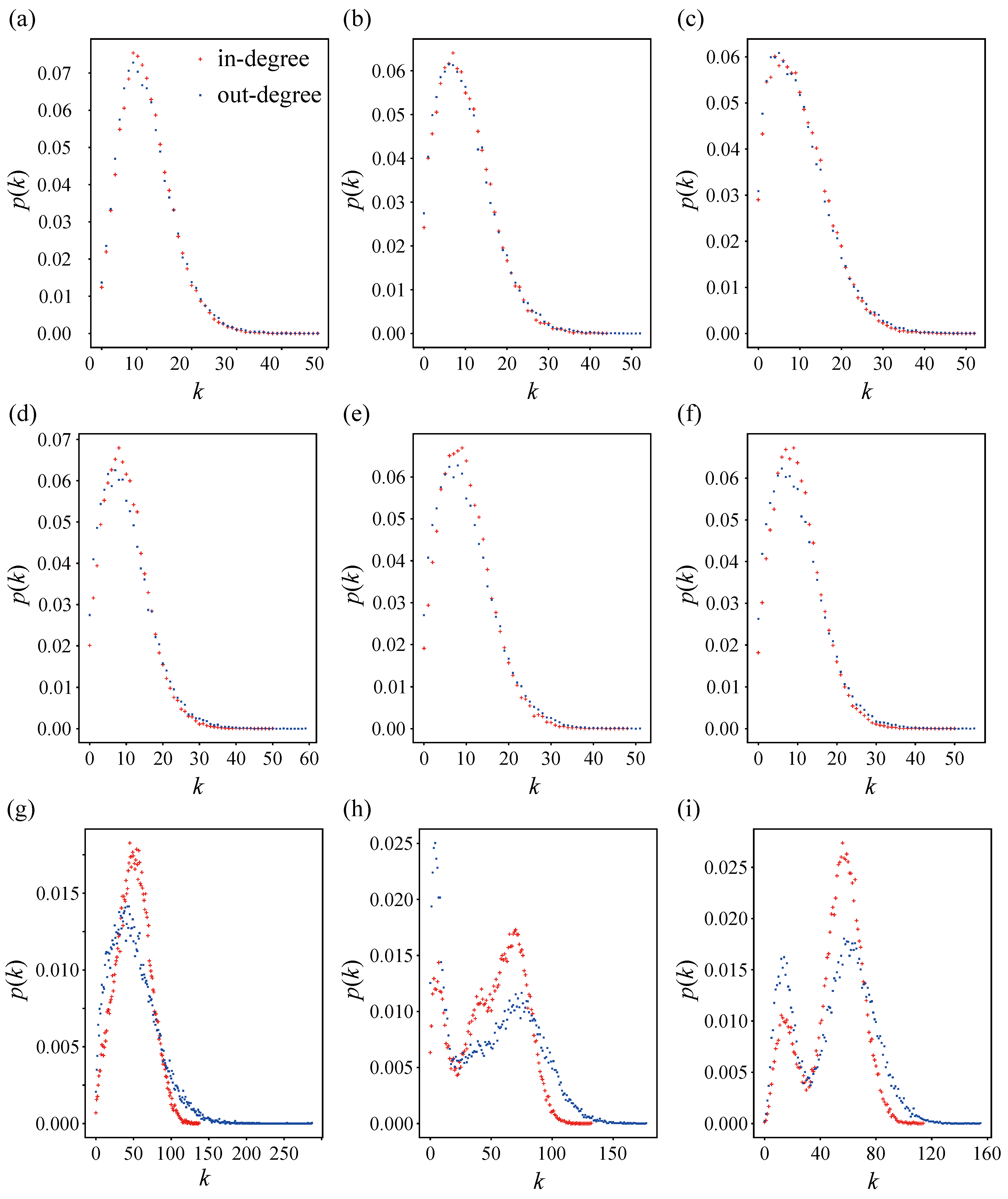
The extended model introduces node-type-specific initial attractiveness parameters, which not only control the asymmetry indices but also shape the emergent degree distributions. We investigated how the degree distribution $p\left(k\right)$ varies through numerical simulations. We observed that the proportion of different types of nodes, as well as their initial attractiveness for in-degrees and out-degrees, does affect the shape of the degree distribution. The key outcomes can be grouped by the number of distinct node types present in the network:

(1)

Single node type. When only one type of node exists, the model reduces to the homogeneous model of [40], and the shape of the degree distribution is determined solely by the single pair of initial attractiveness parameters.

(2)

Two node types. With two functional node types, the shape of degree distribution depends on the mixture of node types and attractiveness disparities.

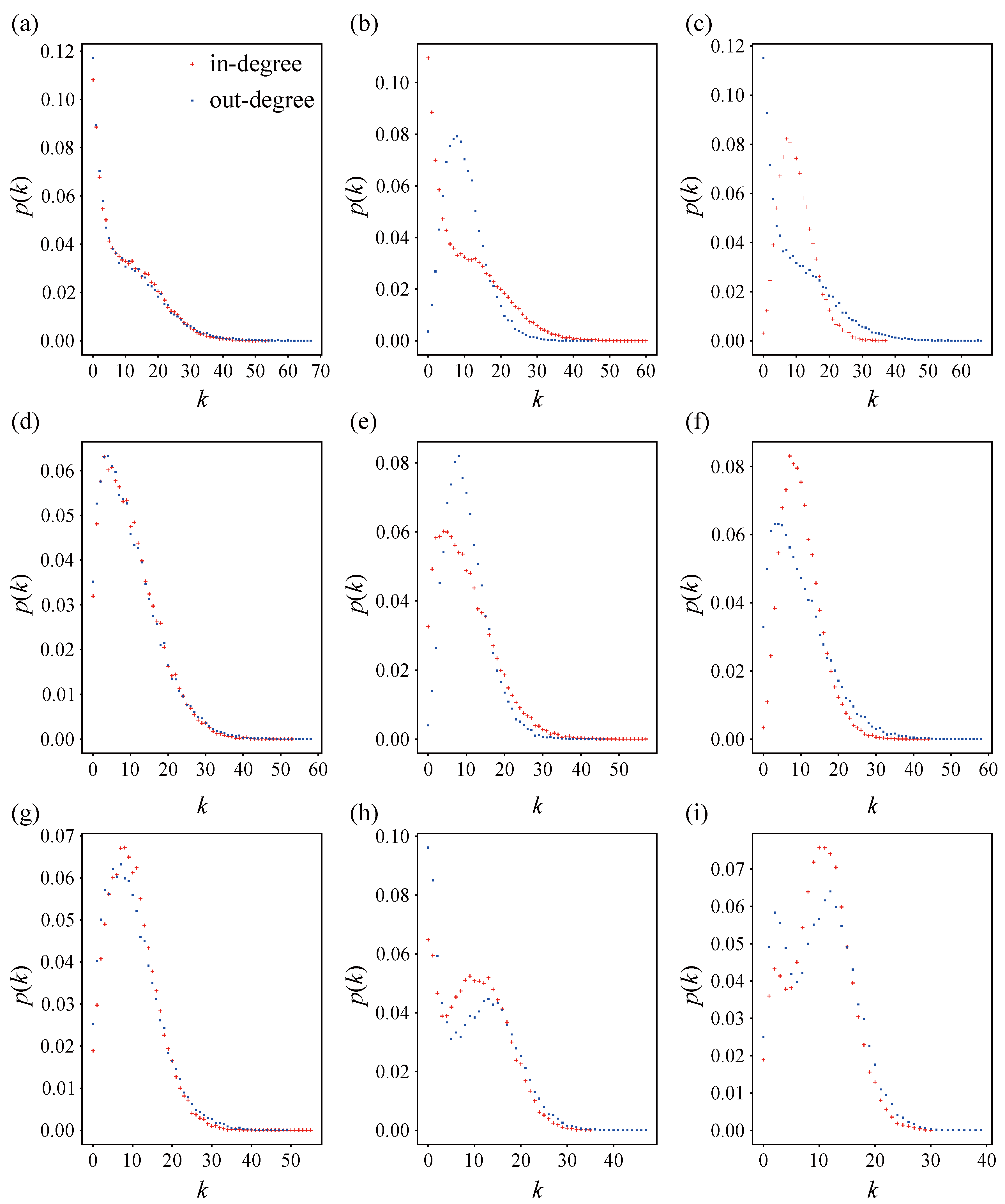
• When the node types are sensory neurons and motor neurons ($s_r>0$, $m_r>0$, and $s_r+m_r=1$), $p\left(k\right)$ for both in-degree and out-degree are similar (Figure 4a,d).
• When the node types are sensory neurons and interneurons ($0<s_r<1$ and $m_r=0$), $p\left(k\right)$ for the out-degree has a peak at the left of the average degree (Figure 4b,e).
• When the node types are interneurons and motor neurons ($s_r=0$ and $0<m_r<1$), $p\left(k\right)$ for the in-degree has a peak at the left of the average degree (Figure 4c,f).

(3)

Three node types. When all three classes are present, the degree distribution exhibits greater diversity.

• If the initial attractiveness values of the three types are all >1 and relatively balanced, $p\left(k\right)$ for both in-degree and out-degree is unimodal and peaks near the average degree (Figure 4g and Figure 5a–g).
• As the disparity among the type-specific attractiveness parameters grows, a secondary peak emerges on the right tail of the distribution (Figure 4h and Figure 5h).
• When the attractiveness differences are extreme—e.g., $a_{\mathrm{out}}$ and $c_{\mathrm{in}}$ are much larger than the other parameters, $p\left(k\right)$ becomes distinctly bimodal, with one peak on each side of the mean degree (Figure 4i and Figure 5i).

Figure 4 and Figure 5 illustrate these trends for networks of $N=300$. The shape of the degree distribution is primarily governed by the relative magnitudes of the type-specific attractiveness parameters, while factors such as the node type proportions ($s_r,m_r$), edge removal probability p, and network density only modulate the distribution mildly; they shift peaks and widths but do not alter the fundamental modality (Figure 4 and Figure 5a–f). Notably, when $a_{out}$, $b_{in}$, $b_{out}$, and $c_{in}$ are much larger than $a_{in}$ and $c_{out}$, $p\left(k\right)$ has a double peak. Increasing the network density (e.g., $E=$ 15,000 vs. $E=3000$) does not eliminate the bimodal distribution; if the attractiveness disparity is sufficiently strong, the double-peak pattern persists (Figure 5g–i). The emergence of bimodal degree distributions can be understood intuitively as follows. Sensory neurons acquire a large number of outgoing edges and very few incoming edges because of their high out-degree initial attractiveness. Motor neurons, due to their high in-degree initial attractiveness, accumulate a large number of incoming edges and very few outgoing edges. Because interneurons possess both high in-degree and high out-degree initial attractiveness, they simultaneously obtain relatively high in-degrees and out-degrees. Consequently, in the in-degree distribution, sensory neurons (low in-degree) separate from motor neurons and interneurons (high in-degree) to form two distinct peaks. In the out-degree distribution, motor neurons (low out-degree) separate from sensory neurons and interneurons (high out-degree) to form two distinct peaks. This bimodal phenomenon is a direct consequence of functional differentiation among the three node types under preferential attachment, reflecting the distinguishability between extreme functional specialization and the intermediate mixed type. These results demonstrate that the extended model can generate a wide repertoire of degree distribution shapes, from unimodal to strongly bimodal, by tuning type-specific initial attractiveness.

3.3.3. Impacts of Node Types and Their Proportions on the Asymmetry Index

Table 5. The asymmetry index (${\alpha }_m$), average clustering coefficient ($C_m$), and average shortest path length ($L_m$) of the model-generated networks in Figure 4.

$\mathit{N}$	300	300	300	300	300	300	300	300	300
$\mathit{E}$	3000	3000	3000	3000	3000	3000	3000	3000	3000
${\mathit{a}}_{\mathit{in}}$	1	1	1	2	2	2	2	2	5
${\mathit{a}}_{\mathit{out}}$	5	5	5	5	5	5	5	10	20
${\mathit{b}}_{\mathit{in}}$	5	5	5	5	5	5	5	20	20
${\mathit{b}}_{\mathit{out}}$	5	5	5	5	5	5	5	20	20
${\mathit{c}}_{\mathit{in}}$	5	5	5	5	5	5	5	10	20
${\mathit{c}}_{\mathit{out}}$	1	1	1	2	2	2	2	2	5
${\mathit{s}}_{\mathit{r}}$	0.5	0.5	0	0.5	0.5	0	0.2	0.2	0.2
${\mathit{m}}_{\mathit{r}}$	0.5	0	0.5	0.5	0	0.5	0.3	0.3	0.3
$\mathit{p}$	0.1	0.1	0.1	0.1	0.1	0.1	0.1	0.1	0.1
${\mathit{\alpha }}_{\mathit{m}}$	0.011	−0.142	0.156	0.007	−0.059	0.071	0.020	0.048	0.025
${\mathit{C}}_{\mathit{m}}$	0.039	0.051	0.052	0.042	0.045	0.045	0.043	0.059	0.039
${\mathit{L}}_{\mathit{m}}$	2.584	2.543	2.530	2.853	2.765	2.770	2.769	2.307	2.763
${\mathit{\alpha }}_{\mathit{Sm}}$	−0.652	−0.517		−0.417	−0.280		−0.444	−0.676	−0.625
${\mathit{\alpha }}_{\mathit{Im}}$		0.233	−0.226		0.162	−0.153	−0.026	−0.033	−0.043
${\mathit{\alpha }}_{\mathit{Mm}}$	0.673		0.538	0.430		0.295	0.405	0.664	0.573

and

Table 6. The asymmetry index (${\alpha }_m$), average clustering coefficient ($C_m$), and average shortest path length ($L_m$) of the model-generated networks in Figure 5.

$\mathit{N}$	300	300	300	300	300	300	300	300	300
$\mathit{E}$	3000	3000	3000	3000	3000	3000	15,000	15,000	15,000
${\mathit{a}}_{\mathit{in}}$	2	2	2	2	2	2	2	2	5
${\mathit{a}}_{\mathit{out}}$	5	5	5	5	5	5	5	10	20
${\mathit{b}}_{\mathit{in}}$	5	5	5	5	5	5	5	20	20
${\mathit{b}}_{\mathit{out}}$	5	5	5	5	5	5	5	20	20
${\mathit{c}}_{\mathit{in}}$	5	5	5	5	5	5	5	10	20
${\mathit{c}}_{\mathit{out}}$	2	2	2	2	2	2	2	2	5
${\mathit{s}}_{\mathit{r}}$	0.1	0.3	0.4	0.2	0.2	0.2	0.2	0.2	0.2
${\mathit{m}}_{\mathit{r}}$	0.1	0.3	0.4	0.3	0.3	0.3	0.3	0.3	0.3
$\mathit{p}$	0.1	0.1	0.1	0.2	0.3	0.4	0.1	0.1	0.1
${\mathit{\alpha }}_{\mathit{m}}$	0.005	0.006	0.007	0.019	0.020	0.021	0.039	0.061	0.033
${\mathit{C}}_{\mathit{m}}$	0.042	0.044	0.044	0.044	0.044	0.044	0.211	0.279	0.194
${\mathit{L}}_{\mathit{m}}$	2.770	2.766	2.793	2.757	2.756	2.763	1.886	1.918	1.894
${\mathit{\alpha }}_{\mathit{Sm}}$	−0.417	−0.418	−0.412	−0.442	−0.436	−0.438	−0.393	−0.609	−0.582
${\mathit{\alpha }}_{\mathit{Im}}$	0.004	0.004	−0.005	−0.032	−0.029	−0.027	−0.018	−0.048	−0.046
${\mathit{\alpha }}_{\mathit{Mm}}$	0.437	0.434	0.433	0.411	0.406	0.408	0.421	0.688	0.575

present the numerical values corresponding to the simulation results shown in Figure 4 and Figure 5. The parameters $s_r$ and $m_r$ control the presence and proportions of the three node classes. The asymmetry indices of the model-generated networks follow the predictable patterns determined by node type composition:

(1)

Sensory and motor neurons ($s_r+m_r=1$): ${\alpha }_{Sm}<0$ and ${\alpha }_{Mm}>0$, which is consistent with the intrinsic functional bias of these types.

(2)

Sensory neurons and interneurons ($m_r=0$): ${\alpha }_{Sm}<0$ and ${\alpha }_{Im}>0$, because the interneurons act as the main recipients when motor neurons are absent.

(3)

Interneurons and motor neurons only ($s_r=0$): ${\alpha }_{Im}<0$ and ${\alpha }_{Mm}>0$, with interneurons acting as the primary output source.

(4)

All three types ($s_r+m_r<1$): ${\alpha }_{Sm}<0$, ${\alpha }_{Mm}>0$, and ${\alpha }_{Im}$ is close to zero or slightly negative, which matches the empirical observations.

The global asymmetry index ${\alpha }_m$ is also sensitive to the proportions of different node types. When only sensory and motor neurons are present and their numbers are balanced, ${\alpha }_m\approx 0$; when one class dominates, ${\alpha }_m$ deviates from zero accordingly. For example, when $0<s_r<1$ and $m_r=0$, ${\alpha }_m$ is affected by $s_r$, with ${\alpha }_m<0$ when $s_r>0.1$; when $0<m_r<1$ and $s_r=0$, ${\alpha }_m$ is affected by $m_r$, with ${\alpha }_m>0$ when $m_r>0.1$. In networks containing all three classes, ${\alpha }_m$ is generally positive within the parameter ranges explored in this study, and its magnitude depends on the relative proportions of the three neuron types.

For comparison, Table 4 lists the metrics of Erdös-Rényi (ER) random networks with identical N and E. ER networks produce asymmetry indices that are several orders of magnitude smaller than those of the model-generated networks, confirming that the extended model captures the directed degree imbalance far better than a purely random null model. The average clustering coefficient $C_m$ is slightly larger than $C_{ER}$ but remains substantially below biological values, while $L_m$ is comparable to both $L_{ER}$ and the real connectomes. These findings confirm that the extended model recapitulates type-specific asymmetry and broad degree distribution features, yet they also highlight its limitations, particularly, its inability to generate high clustering. Therefore, future studies will incorporate additional mechanisms, such as spatial embedding or type-specific wiring rules, to increase the clustering coefficient while preserving the existing features.

4. Discussion

A key characteristic of the extended model is the introduction of three distinct node types, each with its own set of initial attractiveness parameters for incoming and outgoing connections. In biological neural networks, neurons are functionally classified into sensory neurons, interneurons, and motor neurons. As demonstrated in Section 3.1, the asymmetry analysis of these functionally defined neuron classes reveals systematic differences across connectomes. Sensory neurons tend to exhibit negative asymmetry indices (${\alpha }_S<0$), motor neurons tend to exhibit positive asymmetry indices (${\alpha }_M>0$), and interneurons show intermediate values (${\alpha }_I\approx 0$). By selecting type-specific attractiveness parameters, the extended model can reproduce these empirically observed type-specific asymmetry profiles, a capability that homogeneous growth models do not have. Numerical simulations further indicate that the shape of the degree distribution is influenced by the choice of initial attractiveness parameters, node types, and overall network density. Notably, when the initial attractiveness for the out-degree of sensory neurons substantially exceeds that for their in-degree, the probability density function $p\left(k\right)$ of the degree distribution can exhibit a double-peak structure (see Figure 4i and Figure 5h,i). Although this phenomenon emerges from the model dynamics, its theoretical derivation remains an open question, to be addressed in future work.

There are several limitations to the present modeling framework. First, biological neural networks are inherently weighted, where the strength of chemical synaptic connections typically follows truncated power-law distributions [23]. The existing model only generates binary, unweighted edges and does not incorporate mechanisms for weights or plasticity. Extending the framework to accommodate weighted connections—for example, by integrating dynamics inspired by models such as the one proposed in [41]—is an important direction for future study. Second, the model does not incorporate spatial constraints. In biological nervous systems, the physical distance between neurons affects connection probability, and axonal projection ranges are limited. Ignoring spatial embedding may explain the model’s inability to reproduce high clustering coefficients, given that local spatial proximity constitutes a major driver of clustering. Third, the model does not capture developmental mechanisms such as activity-dependent pruning, neurogenesis timing, or axon guidance cues beyond the simplified initial attractiveness parameters. While our aim is to provide a minimal generative framework that reproduces type-specific asymmetry, future work should integrate these biological processes to achieve a more mechanistic understanding of connectome formation.

Additionally, the extended model consistently generates networks with average clustering coefficients that are substantially lower than those observed in real connectomes. Although these values slightly exceed those of Erdös-Rényi random networks, the model still fails to capture the high local clustering characteristic of neuronal networks. This limitation likely stems from the model’s lack of constraints on connectivity patterns between different neuron types. For instance, in real connectomes, sensory neurons preferentially target interneurons, and interneurons themselves exhibit diverse connectivity. To address the low clustering coefficients, future refinements could incorporate type-specific wiring rules that promote local connectivity. For example, one could introduce a triadic closure mechanism, where the formation of a new edge is favored if the two nodes share a common neighbor; alternatively, imposing higher connection probabilities among interneurons, or between functionally related groups, may increase clustering coefficients.

The proposed model is a phenomenological generative framework, which reproduces targeted statistical features (type-specific asymmetry and degree distribution shapes) but does not purport to identify the biophysical or genetic mechanisms that causally drive connectome development. As mentioned in the Introduction, true mechanistic models of neural wiring must integrate spatial constraints [20], gene expression patterns [38,39], and activity-dependent plasticity. The present work serves as a baseline that highlights the necessity of incorporating neuronal types into network growth models, and it provides a minimal framework for doing so.

Despite these limitations, generative models that capture the mesoscale structural features of biological connectomes offer potential insights for the design of artificial neural networks. Previous studies have demonstrated that incorporating connectome-derived topological features, such as the olfactory circuit motifs of Drosophila [42] or the wiring topology of C. elegans [43], can yield efficient architectures for specific machine learning tasks. By providing a systematic method to generate networks with realistic, type-conditioned degree asymmetries, the extended model may serve as a useful tool for exploring how such structural constraints influence information processing in artificial neural networks.

5. Conclusions

This study analyzed type-specific connection asymmetry in biological neural networks and proposed an extended growth model with type-dependent attractiveness parameters to reproduce these observed patterns. While the model successfully captures distinct asymmetry profiles across sensory neurons, interneurons, and motor neurons, it remains a phenomenological baseline. Future integration of spatial constraints and wiring motifs will be essential for gaining mechanistic insights into neural circuit formation.

References

1. Zeng, H.; Sanes, J.R. Neuronal cell-type classification: Challenges, opportunities and the path forward. Nat. Rev. Neurosci. 2017, 18, 530–546. [Google Scholar] [CrossRef] [Scilit] [PubMed]
2. Usoskin, D.; Furlan, A.; Islam, S.; Abdo, H.; Lönnerberg, P.; Lou, D.; Hjerling-Leffler, J.; Haeggström, J.; Kharchenko, O.; Kharchenko, P.V.; et al. Unbiased classification of sensory neuron types by large-scale single-cell RNA sequencing. Nat. Neurosci. 2015, 18, 145–153. [Google Scholar] [CrossRef] [Scilit] [PubMed]
3. Eckstein, N.; Bates, A.S.; Champion, A.; Du, M.; Yin, Y.; Schlegel, P.; Lu, A.K.Y.; Rymer, T.; Finley-May, S.; Paterson, T.; et al. Neurotransmitter classification from electron microscopy images at synaptic sites in Drosophila melanogaster. Cell 2024, 187, 2574–2594.e23. [Google Scholar] [CrossRef] [Scilit] [PubMed]
4. White, J.G.; Southgate, E.; Thomson, J.N.; Brenner, S. The structure of the nervous system of the nematode Caenorhabditis elegans. Philos. Trans. R. Soc. Lond. B Biol. Sci. 1986, 314, 1–340. [Google Scholar] [CrossRef] [Scilit] [PubMed]
5. Cook, S.J.; Jarrell, T.A.; Brittin, C.A.; Wang, Y.; Bloniarz, A.E.; Yakovlev, M.A.; Nguyen, K.C.; Tang, L.T.H.; Bayer, E.A.; Duerr, J.S.; et al. Whole-animal connectomes of both Caenorhabditis elegans sexes. Nature 2019, 571, 63–71. [Google Scholar] [CrossRef] [Scilit] [PubMed]
6. Witvliet, D.; Mulcahy, B.; Mitchell, J.K.; Meirovitch, Y.; Berger, D.R.; Wu, Y.; Liu, Y.; Koh, W.X.; Parvathala, R.; Holmyard, D.; et al. Connectomes across development reveal principles of brain maturation. Nature 2021, 596, 257–261. [Google Scholar] [CrossRef] [Scilit] [PubMed]
7. Jarrell, T.A.; Wang, Y.; Bloniarz, A.E.; Brittin, C.A.; Xu, M.; Thomson, J.N.; Albertson, D.G.; Hall, D.H.; Emmons, S.W. The connectome of a decision-making neural network. Science 2012, 337, 437–444. [Google Scholar] [CrossRef] [Scilit] [PubMed]
8. Ryan, K.; Lu, Z.; Meinertzhagen, I.A. The CNS connectome of a tadpole larva of Ciona intestinalis (L.) highlights sidedness in the brain of a chordate sibling. eLife 2016, 5, e16962. [Google Scholar] [CrossRef] [Scilit] [PubMed]
9. Ivan, L.; Fritsch, P.M.; Nanae, G.; Larisa, N.M.G.; Fetter, R.D.; Schneider-Mizell, C.M.; Truman, J.W.; Marta, Z.; Cardona, A.; Sprecher, S.G. Organization of the Drosophila larval visual circuit. eLife 2017, 6, e28387. [Google Scholar] [CrossRef] [Scilit] [PubMed]
10. Berck, M.E.; Khandelwal, A.; Claus, L.; Hernandez-Nunez, L.; Si, G.; Tabone, C.J.; Li, F.; Truman, J.W.; Fetter, R.D.; Louis, M.; et al. The wiring diagram of a glomerular olfactory system. eLife 2016, 5, e14859. [Google Scholar] [CrossRef] [Scilit] [PubMed]
11. Eichler, K.; Li, F.; Litwin-Kumar, A.; Park, Y.; Andrade, I.; Schneider-Mizell, C.M.; Saumweber, T.; Huser, A.; Eschbach, C.; Gerber, B.; et al. The complete connectome of a learning and memory centre in an insect brain. Nature 2017, 548, 175–182. [Google Scholar] [CrossRef] [Scilit] [PubMed]
12. Zarin, A.A.; Mark, B.; Cardona, A.; Litwin-Kumar, A.; Doe, C.Q. A multilayer circuit architecture for the generation of distinct locomotor behaviors in Drosophila. eLife 2019, 8, e51781. [Google Scholar] [CrossRef] [Scilit] [PubMed]
13. Takemura, S.-y.; Bharioke, A.; Lu, Z.; Nern, A.; Vitaladevuni, S.; Rivlin, P.K.; Katz, W.T.; Olbris, D.J.; Plaza, S.M.; Winston, P.; et al. A visual motion detection circuit suggested by Drosophila connectomics. Nature 2013, 500, 175–181. [Google Scholar] [CrossRef] [Scilit] [PubMed]
14. Scheffer, L.K.; Xu, C.S.; Januszewski, M.; Lu, Z.; Takemura, S.y.; Hayworth, K.J.; Huang, G.B.; Shinomiya, K.; Maitlin-Shepard, J.; Berg, S.; et al. A connectome and analysis of the adult Drosophila central brain. eLife 2020, 9, e57443. [Google Scholar] [CrossRef] [Scilit] [PubMed]
15. Li, F.; Lindsey, J.W.; Marin, E.C.; Otto, N.; Dreher, M.; Dempsey, G.; Stark, I.; Bates, A.S.; Pleijzier, M.W.; Schlegel, P.; et al. The connectome of the adult Drosophila mushroom body provides insights into function. eLife 2020, 9, e62576. [Google Scholar] [CrossRef] [Scilit] [PubMed]
16. Winding, M.; Pedigo, B.D.; Barnes, C.L.; Patsolic, H.G.; Park, Y.; Kazimiers, T.; Fushiki, A.; Andrade, I.V.; Khandelwal, A.; Valdes-Aleman, J.; et al. The connectome of an insect brain. Science 2023, 379, eadd9330. [Google Scholar] [CrossRef] [Scilit] [PubMed]
17. Dorkenwald, S.; Matsliah, A.; Sterling, A.R.; Schlegel, P.; Yu, S.-c.; Mckellar, C.E.; Lin, A.; Costa, M.; Eichler, K.; Yin, Y.; et al. Neuronal wiring diagram of an adult brain. Nature 2024, 634, 124–138. [Google Scholar] [CrossRef] [Scilit] [PubMed]
18. Lin, A.; Yang, R.; Dorkenwald, S.; Matsliah, A.; Sterling, A.R.; Schlegel, P.; Yu, S.-c.; Mckellar, C.E.; Costa, M.; Eichler, K.; et al. Network statistics of the whole-brain connectome of Drosophila. Nature 2024, 634, 153–165. [Google Scholar] [CrossRef] [Scilit] [PubMed]
19. Helmstaedter, M.; Briggman, K.L.; Turaga, S.C.; Jain, V.; Seung, H.S.; Denk, W. Connectomic reconstruction of the inner plexiform layer in the mouse retina. Nature 2013, 500, 168–174. [Google Scholar] [CrossRef] [Scilit] [PubMed]
20. Berry, H.; Temam, O. Modeling self-developing biological neural networks. Neurocomputing 2007, 70, 2723–2734. [Google Scholar] [CrossRef] [Scilit]
21. Varshney, L.R.; Chen, B.L.; Paniagua, E.; Hall, D.H.; Chklovskii, D.B. Structural properties of the Caenorhabditis elegans neuronal network. PLoS Comput. Biol. 2011, 7, e1001066. [Google Scholar] [CrossRef] [Scilit] [PubMed]
22. Reese, T.M.; Brzoska, A.; Yott, D.T.; Kelleher, D.J. Analyzing self-similar and fractal properties of the C. elegans neural network. PLoS ONE 2012, 7, e40483. [Google Scholar] [CrossRef] [Scilit] [PubMed]
23. Zhao, H.; Shao, C.; Shi, Z.; He, S.; Gong, Z. The intrinsic similarity of topological structure in biological neural networks. IEEE/ACM Trans. Comput. Biol. Bioinform. 2023, 20, 3292–3305. [Google Scholar] [CrossRef] [Scilit] [PubMed]
24. Milo, R.; Shen-Orr, S.; Itzkovitz, S.; Kashtan, N.; Chklovskii, D.; Alon, U. Network motifs: Simple building blocks of complex networks. Science 2002, 298, 824–827. [Google Scholar] [CrossRef] [Scilit] [PubMed]
25. Milo, R.; Itzkovitz, S.; Kashtan, N.; Levitt, R.; Shen-Orr, S.; Ayzenshtat, I.; Sheffer, M.; Alon, U. Superfamilies of evolved and designed networks. Science 2004, 303, 1538–1542. [Google Scholar] [CrossRef] [Scilit] [PubMed]
26. Towlson, E.K.; Vértes, P.E.; Ahnert, S.E.; Schafer, W.R.; Bullmore, E.T. The rich club of the C. elegans neuronal connectome. J. Neurosci. 2013, 33, 6380–6387. [Google Scholar] [CrossRef] [Scilit] [PubMed]
27. Barabási, A.L.; Albert, R. Emergence of scaling in random networks. Science 1999, 286, 509–512. [Google Scholar] [CrossRef] [Scilit] [PubMed]
28. Albert, R.; Barabási, A.L. Topology of evolving networks: Local events and universality. Phys. Rev. Lett. 2000, 85, 5234–5237. [Google Scholar] [CrossRef] [Scilit] [PubMed]
29. Dorogovtsev, S.; Mendes, J.; Samukhin, A. Structure of growing networks with preferential linking. Phys. Rev. Lett. 2000, 85, 4633–4636. [Google Scholar] [CrossRef] [Scilit] [PubMed]
30. Krapivsky, P.; Redner, S.; Leyvraz, F. Connectivity of growing random networks. Phys. Rev. Lett. 2000, 85, 4629–4632. [Google Scholar] [CrossRef] [Scilit] [PubMed]
31. Newman, M.E. Clustering and preferential attachment in growing networks. Phys. Rev. E 2001, 64, 025102. [Google Scholar] [CrossRef] [Scilit] [PubMed]
32. Jeong, H.; Néda, Z.; Barabási, A. Measuring preferential attachment in evolving networks. Europhys. Lett. 2003, 61, 567–572. [Google Scholar] [CrossRef] [Scilit]
33. Eom, Y.H.; Fortunato, S. Characterizing and modeling citation dynamics. PLoS ONE 2011, 6, e24926. [Google Scholar] [CrossRef] [Scilit] [PubMed]
34. Bianconi, G.; Barabasi, A. Competition and multiscaling in evolving networks. Europhys. Lett. 2001, 54, 436–442. [Google Scholar] [CrossRef] [Scilit]
35. Ergun, G.; Rodgers, G. Growing random networks with fitness. Phys. A-Stat. Mech. Its Appl. 2002, 303, 261–272. [Google Scholar] [CrossRef] [Scilit]
36. Amaral, L.; Scala, A.; Barthelemy, M.; Stanley, H. Classes of small-world networks. Proc. Natl. Acad. Sci. USA 2000, 97, 11149–11152. [Google Scholar] [CrossRef] [Scilit] [PubMed]
37. Zhu, H.; Wang, X.; Zhu, J. Effect of aging on network structure. Phys. Rev. E 2003, 68, 056121. [Google Scholar] [CrossRef] [Scilit] [PubMed]
38. Barabási, D.L.; Barabási, A.L. A genetic model of the connectome. Neuron 2020, 105, 435–445.e5. [Google Scholar] [CrossRef] [Scilit] [PubMed]
39. Kovacs, I.A.; Barabasi, D.L.; Barabasi, A.L. Uncovering the genetic blueprint of the C. elegans nervous system. Proc. Natl. Acad. Sci. USA 2020, 117, 33570–33577. [Google Scholar] [CrossRef] [Scilit] [PubMed]
40. Zhao, H.; Shi, Z.; Gong, Z.; He, S. Modeling the evolution of biological neural networks based on Caenorhabditis elegans connectomes across development. Entropy 2023, 25, 51. [Google Scholar] [CrossRef] [Scilit] [PubMed]
41. Barrat, A.; Barthélemy, M.; Vespignani, A. Modeling the evolution of weighted networks. Phys. Rev. E 2004, 70, 066149. [Google Scholar] [CrossRef] [Scilit] [PubMed]
42. Dasgupta, S.; Stevens, C.F.; Navlakha, S. A neural algorithm for a fundamental computing problem. Science 2017, 358, 793–796. [Google Scholar] [CrossRef] [Scilit] [PubMed]
43. Bardozzo, F.; Terlizzi, A.; Simoncini, C.; Lio, P.; Tagliaferri, R. Elegans-AI: How the connectome of a living organism could model artificial neural networks. Neurocomputing 2024, 584, 127598. [Google Scholar] [CrossRef] [Scilit]
Figure 1. In-degree versus out-degree of different types of neurons in C. elegans connectomes across development. (a) L1 dataset 1; (b) L1 dataset 2; (c) L1 dataset 3; (d) L1 dataset 4; (e) L2 dataset 5; (f) L3 dataset 6; (g) Adult dataset 7; (h) Adult dataset 8. The light gray line indicates that in-degree is equal to out-degree.
Computation 14 00151 g001
Figure 2. Differences in the asymmetry of different types of neurons in C. elegans connectomes across development.
Computation 14 00151 g002
Figure 3. Schematic illustration of the extended model for N = 20 , M = 50 , a i n = 2 , a o u t = 10 , b i n = 10 , b o u t = 10 , c i n = 10 , c o u t = 2 , s r = 0.2 , m r = 0.3 , and p = 0.1 . Start with N isolated nodes, and divide these N nodes into 3 types where the proportion of each node type is controlled by s r and m r . At each time step, one of two possible events can take place: (i) Add a new directed edge with probability 1 p . The two ends of the new edge are selected using preferential attachment. The new edge is drawn with a red solid line. (ii) Randomly remove an existing edge with probability p ( p < 0.5 ). The removed edge is drawn with an orange dashed line. Note that self-loops and duplicate edges are not allowed.
Computation 14 00151 g003
Figure 4. Numerical simulations investigating the impact of the initial attractiveness of the in-degrees and out-degrees of nodes on the degree distribution of a network where N = 300 , E = 3000 , and p = 0.1 . (ac) The probability density function p ( k ) of networks containing two types of nodes where the initial attractiveness were set as follows: a i n = 1 , a o u t = 5 , b i n = 5 , b o u t = 5 , c i n = 5 , c o u t = 1 . (a) s r = 0.5 , m r = 0.5 ; (b) s r = 0.5 , m r = 0 ; (c) s r = 0 , m r = 0.5 . (df) The probability density function p ( k ) of networks containing two types of nodes where the initial attractiveness were set as follows: a i n = 2 , a o u t = 5 , b i n = 5 , b o u t = 5 , c i n = 5 , c o u t = 2 . (d) s r = 0.5 , m r = 0.5 ; (e) s r = 0.5 , m r = 0 ; (f) s r = 0 , m r = 0.5 . (gi) The probability density function p ( k ) of networks containing three types of nodes, with s r = 0.2 and m r = 0.3 . (g) a i n = 2 , a o u t = 5 , b i n = 5 , b o u t = 5 , c i n = 5 , c o u t = 2 ; (h) a i n = 2 , a o u t = 10 , b i n = 20 , b o u t = 20 , c i n = 10 , c o u t = 2 ; (i) a i n = 5 , a o u t = 20 , b i n = 20 , b o u t = 20 , c i n = 20 , c o u t = 5 . The node types and initial attractiveness for in-degrees and out-degrees can change the shape of the degree distribution. Model results were averaged over 100 realizations.
Computation 14 00151 g004
Figure 5. Numerical simulations investigating the impact of the proportion of different types of nodes, the probability p, and the network density on the network degree distribution and the initial attractiveness of the in-degrees and out-degrees of nodes on the degree distribution of a network. (ac) The probability density function p ( k ) of networks with N = 300 , E = 3000 , a i n = 2 , a o u t = 5 , b i n = 5 , b o u t = 5 , c i n = 5 , c o u t = 2 , and p = 0.1 . (a) s r = 0.1 , m r = 0.1 ; (b) s r = 0.3 , m r = 0.3 ; (c) s r = 0.4 , m r = 0.4 . (df) The probability density function p ( k ) of networks with N = 300 , E = 3000 , a i n = 2 , a o u t = 5 , b i n = 5 , b o u t = 5 , c i n = 5 , c o u t = 2 and s r = 0.2 , m r = 0.3 . (d) p = 0.2 ; (e) p = 0.3 ; (f) p = 0.4 . (gi) The probability density function p ( k ) of networks containing three types of nodes, with N = 300 , E = 15 , 000 , s r = 0.2 , m r = 0.3 , and p = 0.1 , corresponding to (gi) in Figure 4. (g) a i n = 2 , a o u t = 5 , b i n = 5 , b o u t = 5 , c i n = 5 , c o u t = 2 ; (h) a i n = 2 , a o u t = 10 , b i n = 20 , b o u t = 20 , c i n = 10 , c o u t = 2 ; (i) a i n = 5 , a o u t = 20 , b i n = 20 , b o u t = 20 , c i n = 20 , c o u t = 5 . Results for the extended model were averaged over 100 realizations.
Computation 14 00151 g005