Article

Investigation of Decomposition Techniques for Characterizing Complex Vortex Structures in MVG-Controlled Boundary Layer


1
Department of Mathematics, Brandeis University, Waltham, MA 02453, USA
2
Department of Mathematics, Yale University, New Haven, CT 06520, USA
3
Department of Mathematics and Statistics, University of Maryland Baltimore County, Baltimore, MD 21250, USA
4
Department of Mathematics and Statistical Sciences, Jackson State University, Jackson, MS 39217, USA
5
Department of Mathematics, West Texas A&M University, Canyon, TX 79016, USA
*
Author to whom correspondence should be addressed.
Computation 2026, 14(6), 122; https://doi.org/10.3390/computation14060122
Submission received: 17 April 2026 / Revised: 12 May 2026 / Accepted: 22 May 2026 / Published: 25 May 2026
(This article belongs to the Special Issue Advances in Computational Methods for Fluid Flow—2nd Edition)

Abstract

Accurate characterization of coherent vortex structures in high-speed turbulent boundary layers presents a persistent challenge due to the flow’s high dimensionality and nonlinear dynamics. This study investigates an optimized decomposition framework that integrates modal decomposition techniques with a novel vortex identification strategy to extract dynamically significant features. The numerical solution from a previously conducted high-fidelity simulation of MVG-controlled supersonic flow serves as the testbed. Principal Component Decomposition and Non-negative Matrix Factorization are applied across multiple flow variables to evaluate their effectiveness in isolating coherent structures. The results show that, across the velocity-based cases, 3–4 modes capture 70% of the TKE with MSE about 0.1, while the Liutex case requires 14 modes but achieves a lower MSE of about 0.04. Overall, using the same number of modes yields similar reconstruction performance across all cases. The influence of various normalization and rescaling methods on decomposition performance is also examined. Optimization is guided by two primary criteria: the interpretability of spatial modes and MSE in reconstructing vortex structures. By employing low-rank matrix representations, this optimization study aims to enhance interpretability and reduce computational costs. This approach establishes a mathematically rigorous and efficient platform for analyzing vortex dynamics, achieving significant dimensionality reduction while preserving key features of turbulent transport.

1. Introduction

Understanding vortex structures is essential for making sense of complex fluid flows, especially in high-speed environments where turbulence and instabilities dominate. These swirling regions of concentrated vorticity act as the building blocks of flow organization, influencing how energy moves across scales and how momentum and heat are transported. In high-speed flows, vortex stretching and intensification govern the cascade of energy from large to small scales, a phenomenon central to the Kolmogorov turbulence framework [1]. Coherent vortical structures, such as hairpin vortices and vortex rings, not only influence momentum and heat transport but also dictate the onset and evolution of instabilities like Kelvin–Helmholtz waves, which are critical in shear layers and boundary transitions [1,2]. By studying how these structures evolve and interact, researchers can better predict and control flow behavior in applications ranging from aerospace design to environmental modeling. Vortex dynamics, in this sense, provides a conceptual framework that bridges the gap between chaotic motion and coherent patterns in fluid systems [2].
In recent decades, matrix decomposition-based dimension reduction techniques have become important analytical tools in fluid dynamics, enabling researchers to extract coherent structures, reduce computational complexity, and build interpretable models from complex fluid flows, such as turbulent boundary layers. Among the most widely adopted methods is Proper Orthogonal Decomposition (POD) [3,4], which identifies dominant energetic modes in turbulent flows, enabling reduced-order modeling and efficient simulation, has been extensively applied to understand the complex flow structures. Building on this, Balanced POD and Balanced Truncation [5,6] incorporate system dynamics to better capture input–output behavior, which is especially valuable for flow control applications. The emergence of Dynamic Mode Decomposition (DMD) [7,8] marked a shift toward data-driven analysis, allowing researchers to extract coherent spatiotemporal structures and modal growth rates directly from snapshots of flow fields. More recently, nonlinear approaches such as kernel PCA (Principal Component Analysis) [9], autoencoders [10], and manifold learning [11] have expanded the toolkit, revealing low-dimensional representations of fluid phenomena that linear methods may miss. These methods not only reduce computational cost but also enhance physical insight, making them central to modern efforts in modeling, control, and understanding of complex flows.
Micro-vortex generators (MVGs) have gained prominence as compact, passive devices for controlling shock/boundary layer interactions (SBLIs) in high-speed aerodynamic flows [12,13]. Typically sized to span between 10% and 80% of the local boundary layer thickness, MVGs are designed to produce pairs of counter-rotating streamwise vortices that redistribute momentum within the near-wall region. This special vortex pattern enhances the energy of low-speed fluid near the surface, helping to suppress separation and maintain flow attachment in the presence of adverse pressure gradients. Unlike larger or more intrusive control mechanisms, MVGs offer the advantage of minimal drag increase and can be seamlessly embedded into aerodynamic surfaces such as wings, engine inlets, and nozzles. Their effectiveness has been demonstrated across a range of configurations, making them a practical solution for improving flow stability and performance in supersonic and transonic regimes [14]. In our earlier studies [15,16,17], simulations explored supersonic boundary layers influenced by MVGs across Mach numbers 1.5–4.5. The analysis identified complex vortex structures, especially ring-like vortices, which significantly affect SBLI and alter ramp shock dynamics. A V-shaped separation zone was detected along the wall, resulting from the interplay between these vortices and the ramp shock, aiding flow separation reduction at the ramp corner. These findings highlight the paramount role of MVG-induced vortex structures in controlling high-speed boundary layers.
This study investigates the application of machine learning-based dimensionality reduction techniques, specifically PCA and Non-negative Matrix Factorization (NMF) [18], to high-fidelity numerical simulations of vortex structures generated by MVGs in high-speed aerodynamic flows. These methods offer complementary approaches to uncovering low-dimensional representations of complex flow fields: PCA identifies orthogonal modes that capture variance across the dataset, while NMF provides additive, parts-based decompositions that preserve physical interpretability. To enhance the fidelity of vortex characterization, we will systematically evaluate different flow variables, such as velocity components, density, pressure, and vortex identification variables, as inputs to the decomposition process. By comparing the resulting modal structures and reconstruction accuracy, we aim to identify an optimized framework for vortex-based dimensionality reduction that reduces the error in the reconstruction of the coherent vortex structure by the dominant components. Moreover, applying dimensionality reduction to fully three-dimensional turbulence, such as vortex structures in MVG-induced high-speed flows, is rigorous because of the complex, multi-scale, and chaotic nature inherent in any flow field. Most previous studies have either focused on simpler, lower-dimensional datasets or employed standard linear methods (e.g., PCA on 2D slices), leaving a gap in the literature for systematic exploration using techniques like NMF in full three-dimensional turbulent contexts. This approach not only facilitates reduced-order modeling but also deepens physical insight into the dynamics of MVG-induced vortices within turbulent boundary layers.
In this study, after introducing the paper in Section 1, the remainder is organized as follows: Section 2 details the two dimension reduction methods we selected—PCA and NMF—and the process of how we applied them on the data of the MVG-controlled boundary layer, Section 3 and Section 4 present the results and discussion, and Section 5 offers concluding remarks.

2. Numerical Methods

This study utilizes previously generated numerical data from simulations of supersonic ramp flow controlled by micro-vortex generators (MVGs), conducted within a computational domain defined by Mach 2.5 and a Reynolds number of 5760. In this simulation, the MVG trailing edge is set at a 70° inclination, while all other geometric parameters follow those used in prior experimental studies. The inlet boundary layer thickness is prescribed as 2h (h is the height of the MVG), consistent with both experimental measurements and earlier simulations. At the wall, adiabatic, zero-pressure-gradient, no-slip conditions are enforced. A non-reflecting boundary condition is applied along the upper boundary to suppress spurious wave reflections, and periodic conditions are imposed in the spanwise direction. To better resolve vortex interactions, particularly the ring-like structures generated by the MVG, a low turbulence intensity inlet profile is specified. A non-reflecting outflow boundary condition is also used to maintain numerical stability. The numerical results show that two counter-rotating streamwise vortices are enclosed by a train of ring-like (Ω-shaped) vortices generated behind the MVG, which subsequently propagate downstream and evolve to a very complicated 3D vortex structure (Figure 1). Detailed descriptions of the simulation setup, validation procedures, and flow analysis are available in references [15,16,17]. For the present investigation, a small subdomain was extracted to focus on localized vortex dynamics. Figure 1 illustrates the subdomain’s location and the coherent vortex structures contained within it.

2.1. PCA/POD

Proper Orthogonal Decomposition (POD), which is mathematically equivalent to Principal Component Analysis (PCA), can be viewed as PCA applied to CFD data such as velocity, pressure, or vorticity fields; POD is a dimensionality reduction technique that represents a turbulent flow as a linear combination of spatial modes and associated time-dependent coefficients. It can be used to extract dominant orthogonal modes from data using eigenvalue or singular value decomposition. The leading modes therefore capture the most energetic features of the flow, making POD an effective tool for reduced-order modeling and flow analysis.
In practice, the POD modes (spatial basis) are obtained from the eigenvalue problem of the covariance matrix ( C ) given by:
C   =   1 m 1 U T U
with U being the snapshot matrix of flow variables (usually the zero-mean velocity fluctuations). The eigenvalues of this matrix rank each mode’s contribution to the TKE (turbulent kinetic energy), enabling efficient dimensionality reduction by retaining only the most energetic modes. This eigenvalue problem is commonly solved using Singular Value Decomposition (SVD; see Equation (2)), which produces spatiotemporal decomposition, yielding an orthonormal spatial basis and the associated temporal coefficients.
U = L Σ R T
For the spatial basis decomposition, the orthonormal spatial basis of the snapshot matrix is A = L Σ and the corresponding temporal modes or coefficients are Φ = R .
The spatial modes are time-independent, representing coherent structures present across the flow field, and are ordered by their energetic contribution. For any given number of modes r , POD provides the best low-rank approximation of the turbulent flow. This energy-optimal property is what makes POD particularly valuable for analyzing and modeling coherent vortex structures in complex, high-dimensional flows.

2.2. NMF

Non-negative Matrix Factorization (NMF) is another dimensionality reduction method that approximates a given non-negative matrix U (with m rows and n columns) as the product of two smaller non-negative matrices W and H:
U m × n = W m × p · U p × n , p < m i n { m , n } .
One of the most widely used algorithms for NMF is the method proposed by Lee and Seung [18], which finds the two decomposed matrices by first initializing them to be some positive matrices and then iteratively applying the following multiplicative update rule
H i j n + 1 H i j n ( ( W n ) T U ) i j ( ( W n ) T W n H n ) i j ,   W i j n + 1 W i j n ( U ( H n + 1 ) T ) i j ( W n H n + 1 ( H n + 1 ) T ) i j   ,  
until the squared Frobenius norm U W H 2 is minimized. It follows that if u i and h i are the i th columns of U and H , respectively, then
u i W h i
Hence, the matrix W can be viewed as a “basis” for U , since each column of U can be expressed as a linear combination of the columns of W , with the coefficients given by the corresponding column of H . In particular, if U is the snapshot matrix consisting of velocity fluctuation, the columns of W are the spatial modes [19].
Unlike POD, the spatial modes are not constrained to be orthonormal, providing greater flexibility in the structures that are being captured [20,21]. Furthermore, non-negativity forces additive combinations because subtraction cannot occur, and therefore NMF learns a part-based representation of the original matrix [22].
To match a similar notion of TKE, we calculate the variance as
U W H 2 | | U | | 2 ,
where the norms are the Frobenius norms.

2.3. Application of Decomposition on Vortex Structure in Complex Fluid Flows

To better visualize and identify multi-scale vortices in complex flows, the newly developed vortex identification method, Liutex [23,24], which can capture both axes and the magnitude of local fluid rotation accurately, is used in this study.
Liutex is considered superior to traditional vortex identification methods (such as Q , λ 2 , or Δ ) because it directly extracts the true local rotational motion of the fluid, rather than relying on indirect indicators. The key advantage is that Liutex mathematically isolates rigid-body rotation, removing contamination from shear, stretching, and other non-rotational components that often mislead classical criteria [23,24,25]. It uses RS decomposition to separate non-dissipative rigid rotation from dissipative shear as shown
ω = R + S  
R = ω · r ω · r 2 4 λ c i 2 r
where r is the real eigenvector of v and ω · r > 0 . Let R   =   [ L X ,   L Y ,   L Z ] , where L X , L Y , L Z are the Liutex components.
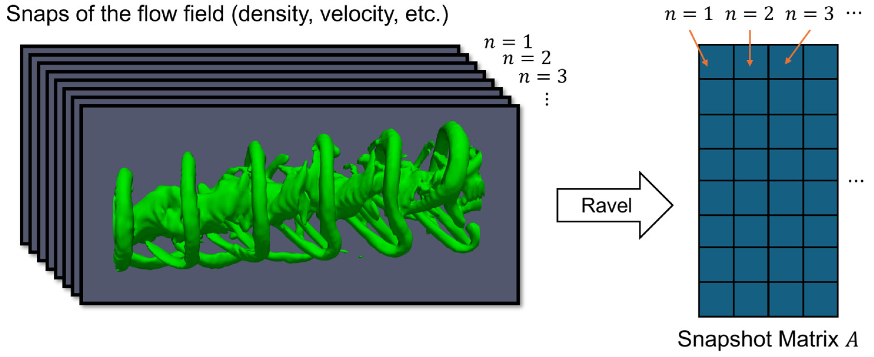
To prepare numerical data from a CFD simulation for further analysis, the output is typically saved at discrete timesteps, with each file capturing the full 3D spatial distribution of key flow variables—such as velocity components, density, and energy—corresponding to a specific moment in time. These volumetric datasets are then processed by unraveling the 3D arrays into 1D vectors (see Figure 2), effectively flattening the spatial information while preserving the variable relationships. By stacking these 1D arrays across all timesteps and variables, we construct a large 2D matrix where each row represents a spatial point and each column corresponds to a particular variable at a given time. This transformation facilitates efficient data handling, visualization, and application of machine learning or statistical techniques for deeper insights into the flow dynamics.

3. Numerical Results

In this study, to explore the optimization of matrix decomposition and reconstruction on vortex structures, combinations of different flow variables and different normalization methods were used.

3.1. POD/PCA with Different Flow Variables

Table 1 gives all the eight cases with different variables used in the POD/PCA.
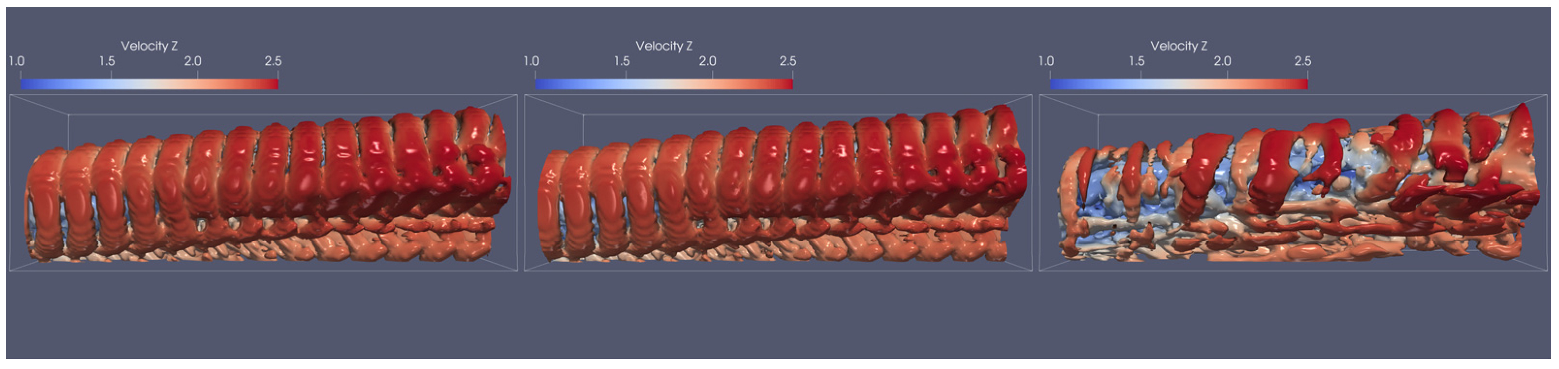
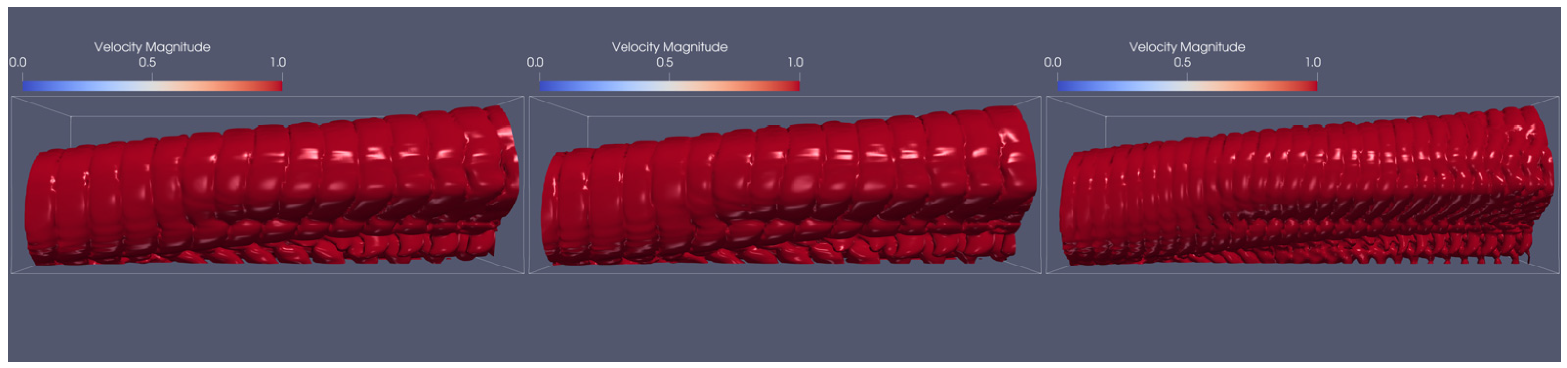
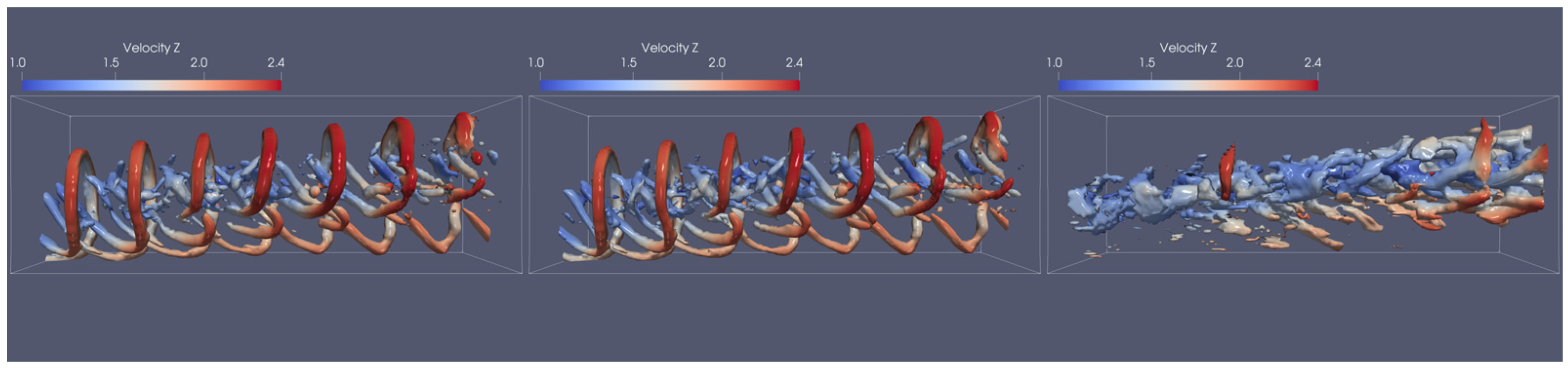
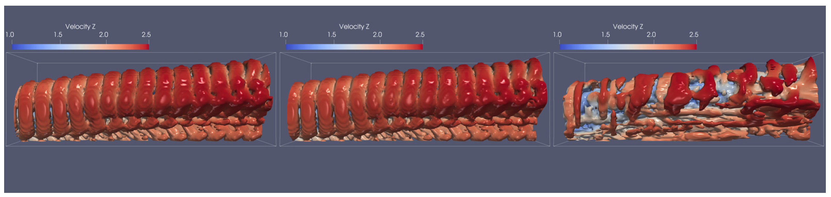
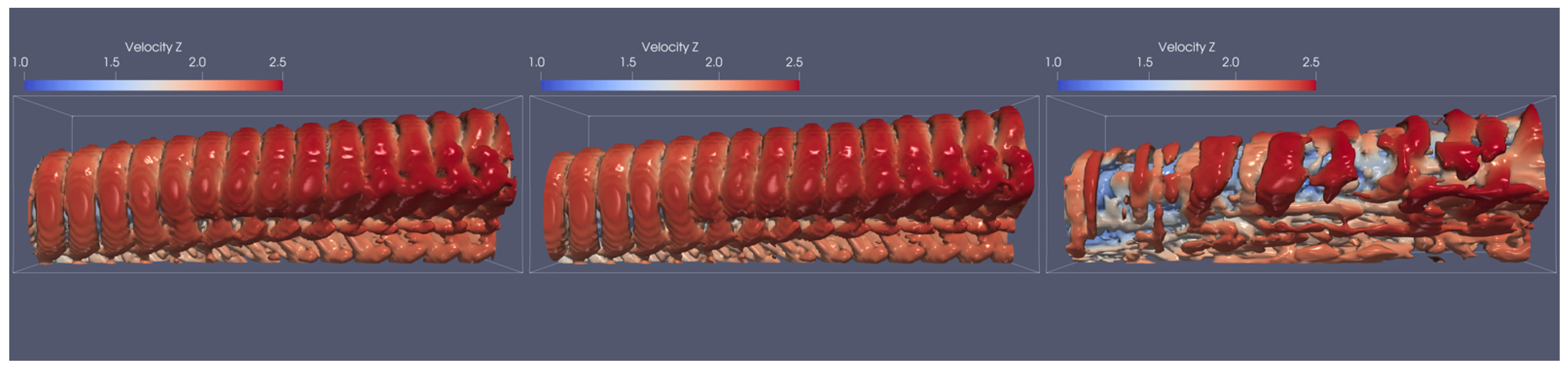
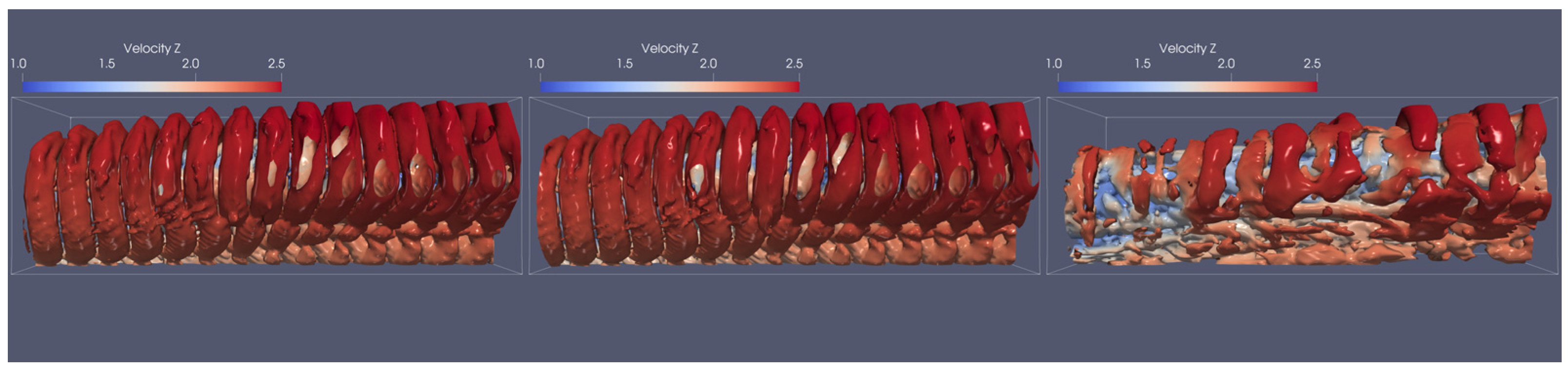
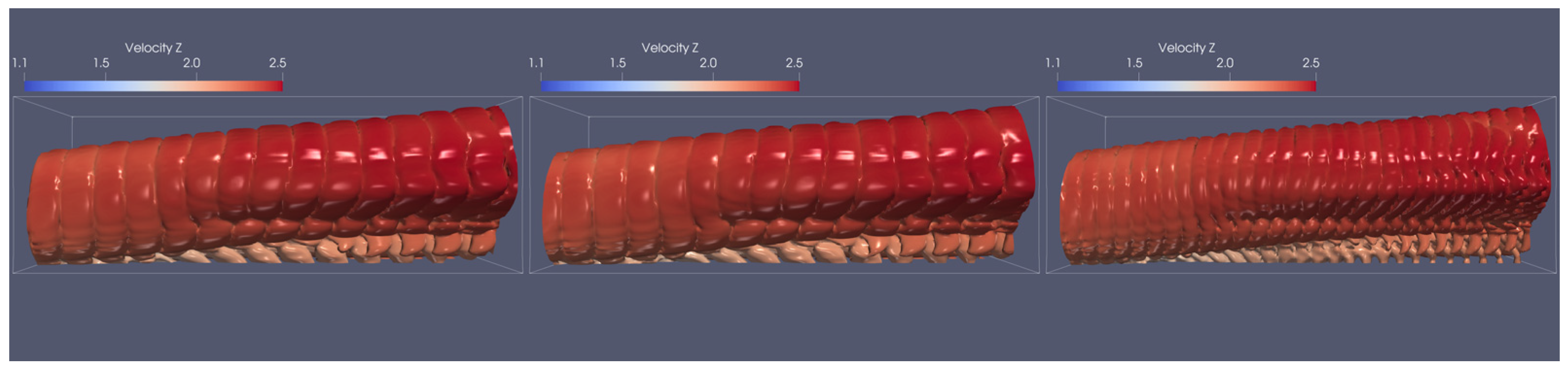
The first three spatial modes extracted from each case are shown in Figure 3, Figure 4, Figure 5, Figure 6, Figure 7, Figure 8 and Figure 9. Instead of the original variables, the converted iso-surface of Liutex, which illustrates the vortex structures, are shown in these figures. POD orders the modes so that these modes capture the largest possible fraction of the total fluctuating energy, with each subsequent mode capturing the maximum remaining energy subject to orthogonality constraints. The first three modes in each case reflect the dominant large-scale structure, consistent with the most energetic coherent motions in the flow. Together, these modes account for the bulk of the variance retained in the reduced-order model, while higher modes (not listed in this paper) contribute progressively finer details at lower energy levels.
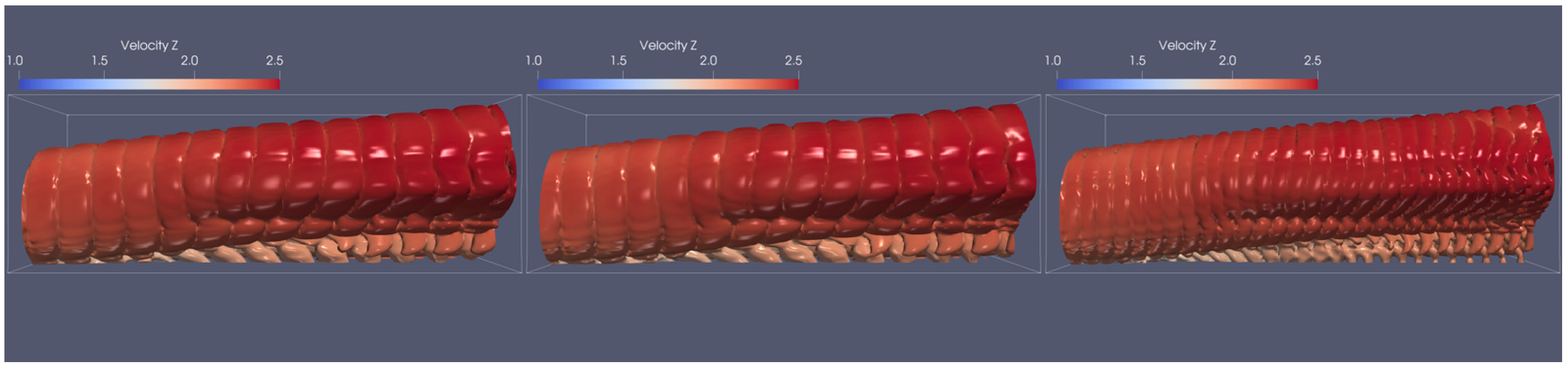
The regenerated vortex structure (iso-surfaces of Liutex) in the spatial modes of Cases 1–6, which involve the momentum components ρ u , ρ v , ρ w , or the velocity components u ,   v ,   w , were observed similar to each other. POD involving Liutex components ( L X ,   L Y ,   L Z ) produce more spatial modes that follow a Fourier-sequel frequency pattern. For Cases 1–6, the first three spatial modes share similar large-scale features, with only minor variations in the small-scale structures. Case 7, however, displays noticeably different modal behavior. Its spatial modes reveal more tightly connected ring-like vortices, and the third mode shifts immediately to a high-frequency structure, distinguishing it from the other cases. Generally, higher-index spatial modes have higher “spatial frequency” in that they have more “rings” but with shorter length, similar to how higher-index trigonometric basis functions, which have higher frequencies and hence more oscillations. What this means for vortex structures is that lower-index spatial modes tend to capture broad, coherent structures, while higher-index modes often contain finer-scale patterns. Although only the first three spatial modes were shown, this trend generally holds across the remaining modes in all cases as well. Interestingly, all the spatial modes from POD involving velocity components appear nearly identical.
In addition, spatial modes involving only Liutex components were generally smoother and well-behaved compared to their velocity counterparts. Whereas the velocity modes began to display incoherent structure after the first two, the Liutex components modes started at five.
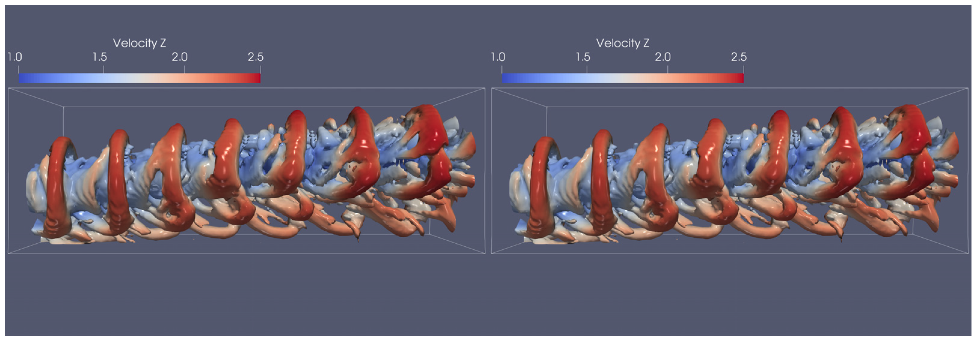
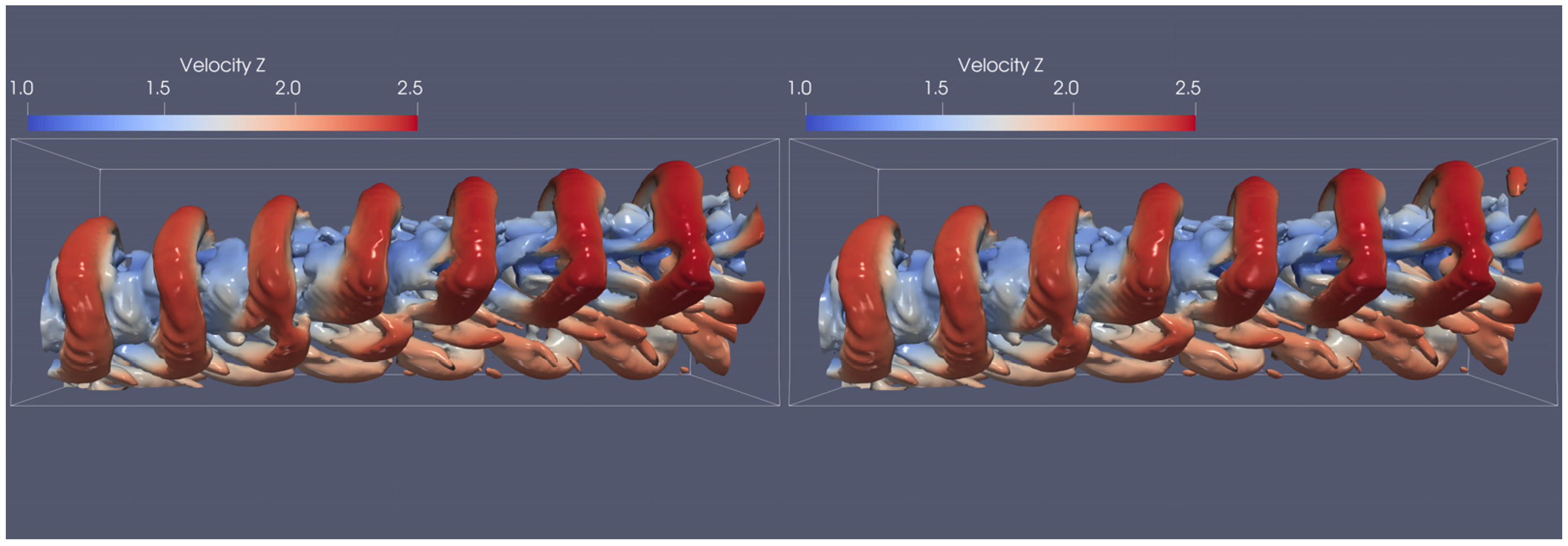
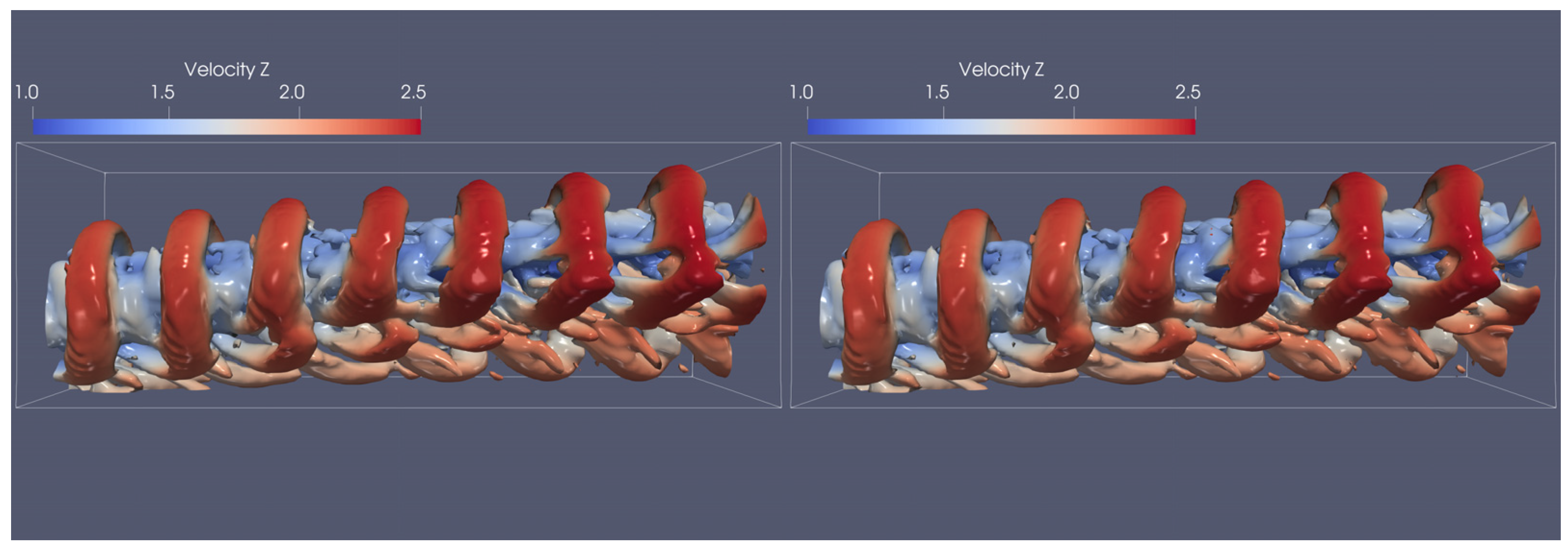
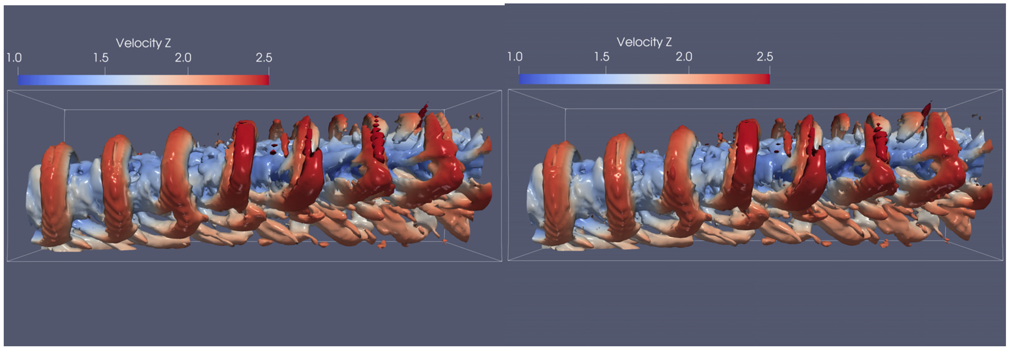
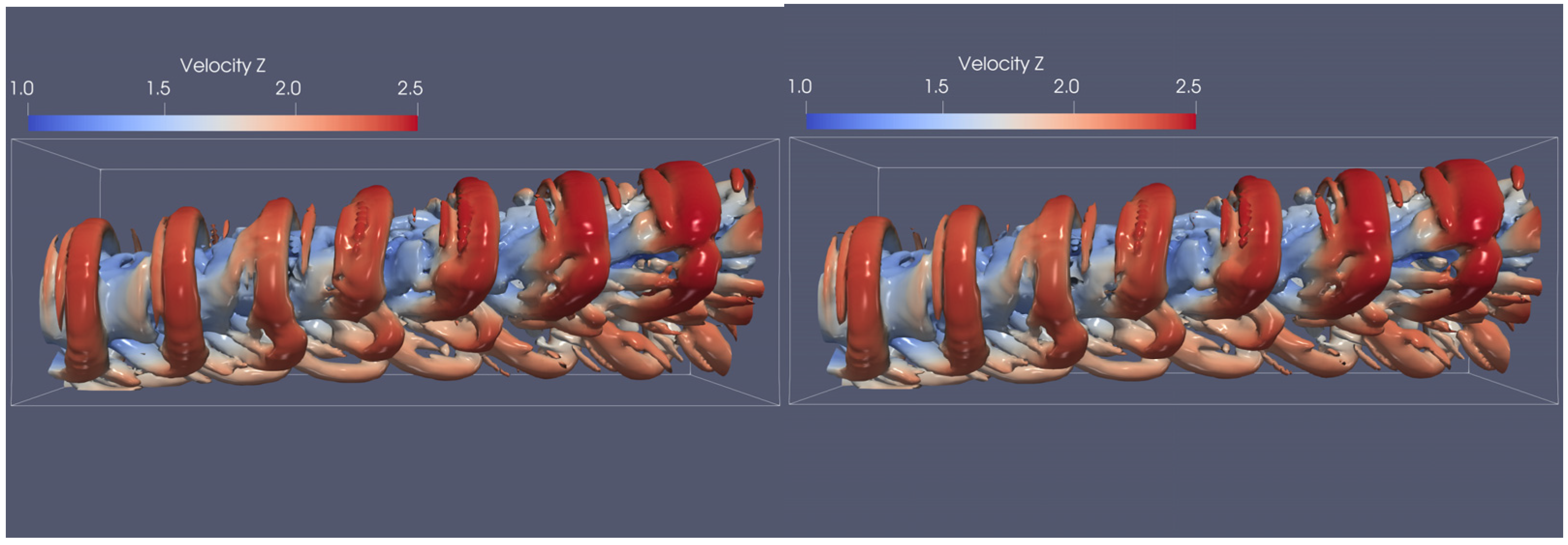
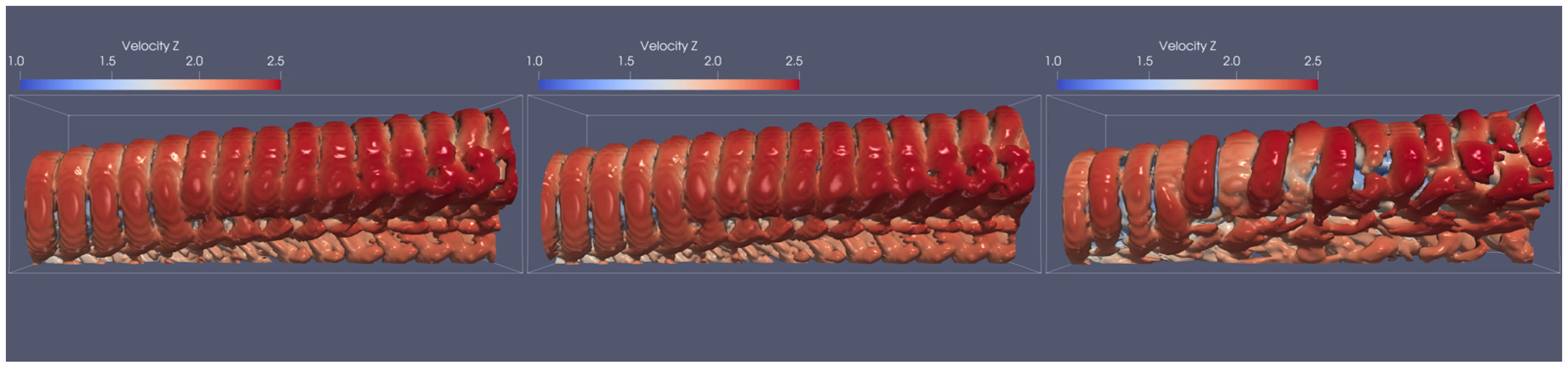
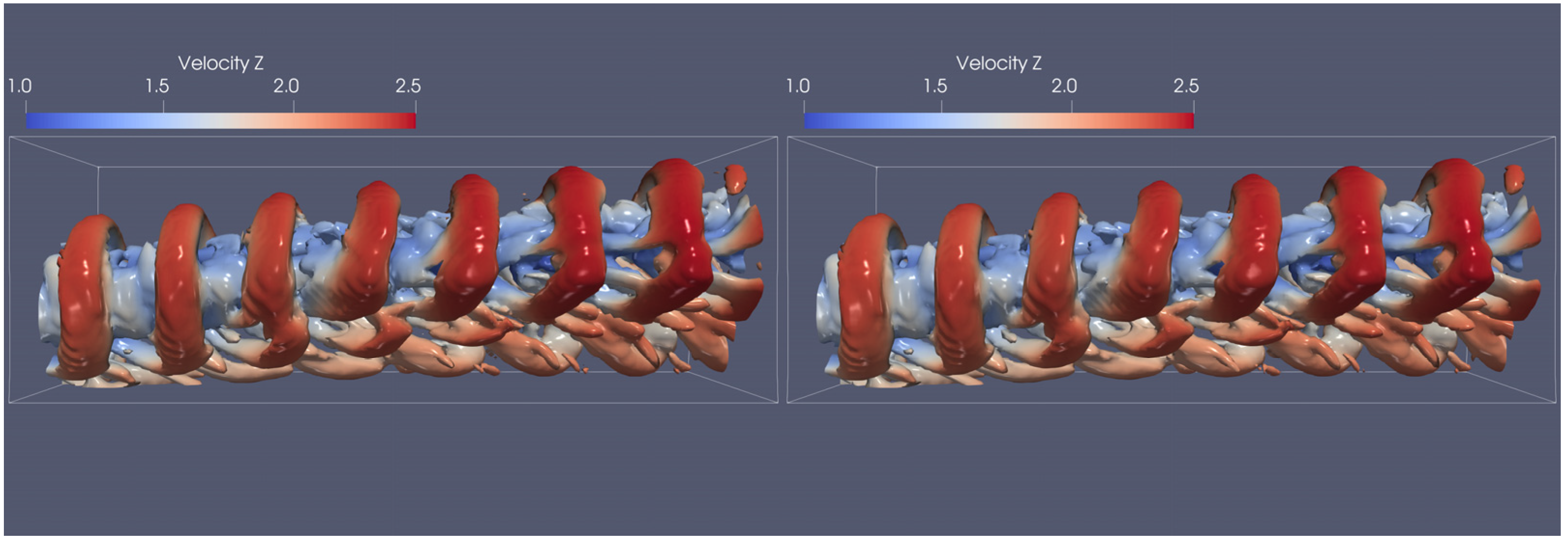
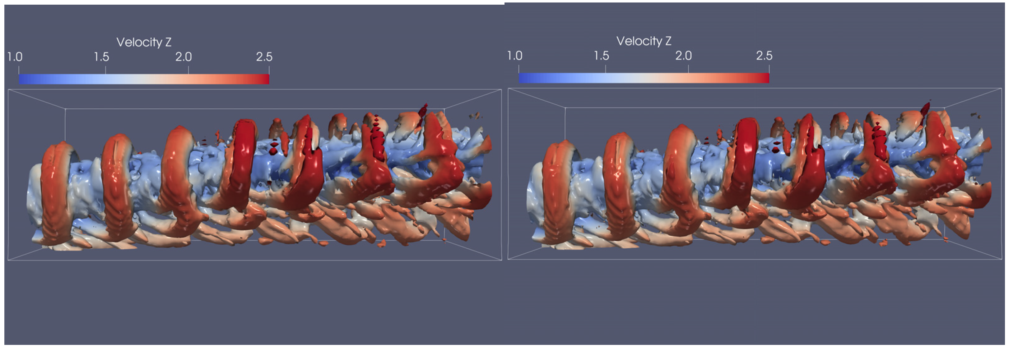
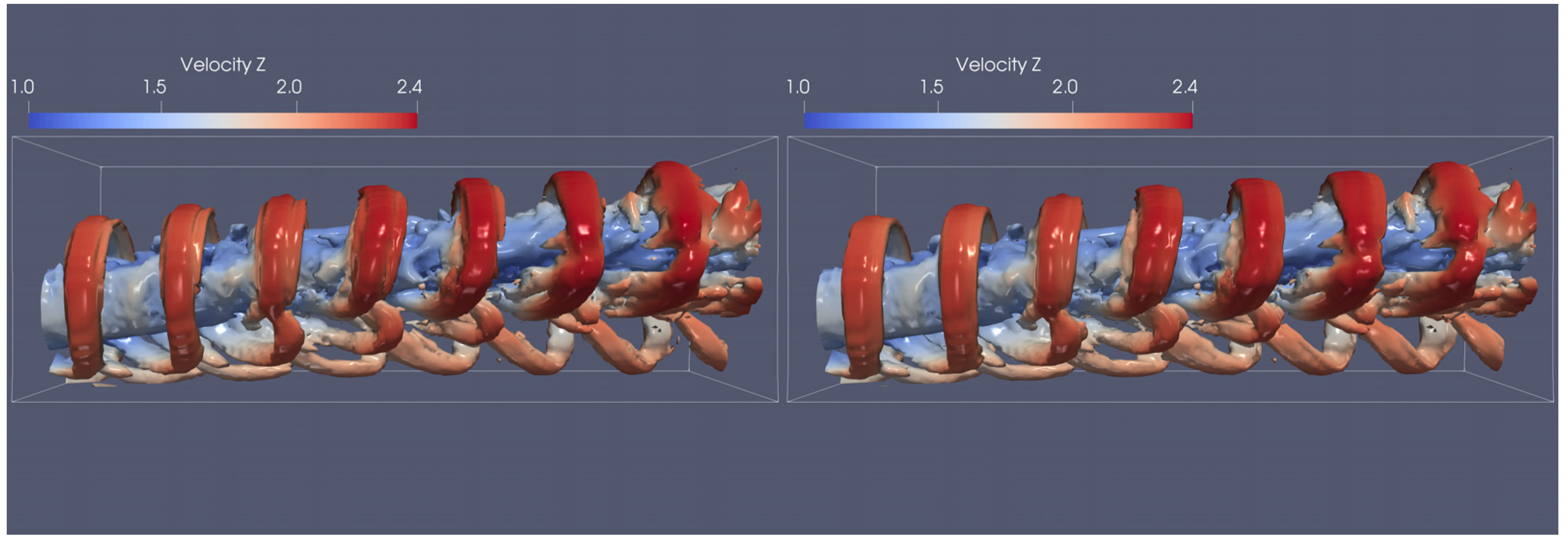
Figure 10 shows the vortex structure from the original simulation data at timesteps 199,900 and 200,000 in our LES simulation [15]. Figure 11, Figure 12, Figure 13, Figure 14, Figure 15, Figure 16 and Figure 17 show the reconstructed vortex structure from the spatial modes with 70% TKE conserved and the corresponding time coefficients for all the cases at the same timesteps. The vortex structures were fully developed at these timesteps in the simulation and are expected to retain the cumulative statistical and dynamical properties of the flow, making them suitable for assessing the quality of the reduced-order reconstruction. In all cases, residual discrepancies, interpreted as pseudo-vortices, are observed in the reconstructions. These errors are referable to POD truncation, in which only a subset of the most energetic modes that are sufficient to capture 70% of TKE is retained for reconstruction. By reconstruction, the discarded higher-order modes contain smaller amounts of total energy but can still encode fine-scale spatial or temporal variability that, when omitted, manifests as localized or oscillatory deviations in the reconstructed field.
Overall, Cases 1, 2, 3, and 4 offer the best balance between physically meaningful spatial modes and smooth reconstruction with the least pseudo-vortices. Results from cases involving momentum and Liutex components (Cases 5, 6, and 7) produce relatively more pseudo-vortices. However, the pseudo-vortices become less observed when more spatial modes are included in the reconstruction. Analysis of Figure 13 and Figure 14, together with Figure 15 and Figure 16, shows that the additional total energy introduced into the system does not affect the orthogonal spatial modes produced by the POD. Consequently, the corresponding reconstructions exhibit the same structures, confirming that the POD modes are insensitive to this energy adjustment.
Table 1 presents MSE (the Mean Squared Error) as a quantitative benchmark for evaluating the reconstruction accuracy of various decomposition frameworks at 70% TKE threshold. However, since Case 7 reaches the same TKE threshold using 14 modes, we uniformly apply 14 modes across all cases to maintain a fair basis for comparison. and a fixed 14-mode count. The data reveals that Case 7, utilizing Liutex components, achieves the lowest MSE of 0.04 at 70% TKE; however, it requires significantly more modes than other cases to reach that energy level. When the number of modes was fixed, the MSE values were of the same magnitude across all cases. Although MSE provides a mathematical baseline for error, it is not an infallible indicator of physical fidelity. Despite its role in guiding optimization, lower MSE values do not always prevent pseudo-vortices.

3.2. PCA/POD with Different Normalization (Rescaling) Method

Preprocessing flow data is a critical step to ensure the robustness and interpretability of decomposition or dimensionality reduction techniques, particularly those sensitive to data scaling such as PCA/POD. The numerical data from our prior simulation was dimensionless and centered. In this section, extra normalization strategies like standard normalization (which adjusts each variable to zero mean and unit variance) and min-max normalization (which maps every variable to [−1, 1] except L X , L Y , and L Z , which are mapped to [0, 1]) are employed to harmonize the influence of variables with differing physical units or magnitudes. Generally, standard rescaling preserves the relative structure of the fluctuation field and therefore does not fundamentally alter the spatial modes obtained from POD/PCA, while min-max normalization redistributes values within a fixed interval, altering the relative weighting of local extrema and compressing or stretching specific portions of the data range. In this study, we applied both normalization/scaling methods independently, recognizing that combining multiple normalization schemes on the same dataset can distort the statistical properties of the fluctuations and compromise physical interpretability. This approach enabled a systematic assessment of how each preprocessing method affects the resulting modal structures and the accuracy of flow field reconstruction.
Table 2 and Table 3 examine the effects of min–max and standard normalization, respectively. Across Cases 1–6, the MSE at 70% TKE remains consistently within approximately 0.10–0.12, matching the baseline values reported in Table 1. The fixed-mode reconstructions (14 modes) also continue to produce uniformly lower errors, reinforcing that the truncation level has a stronger influence on reconstruction accuracy than the choice of normalization. Although Case 7 shows a slight change in the 14-mode MSE, the additional normalization (rescaling) produces virtually no meaningful differences in the remaining values compared with Table 1.
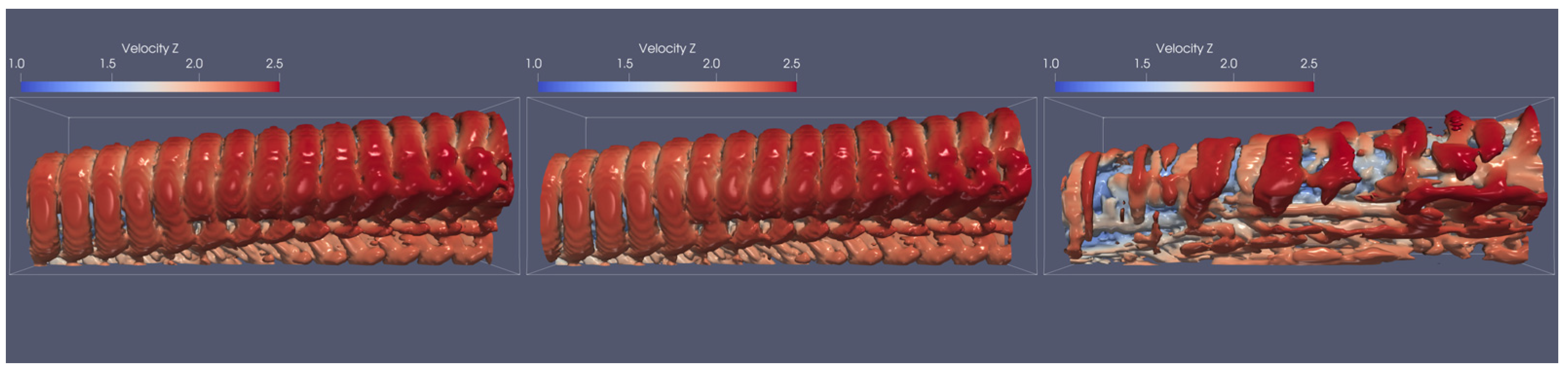
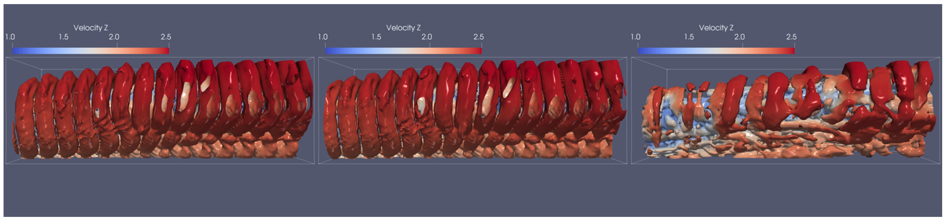
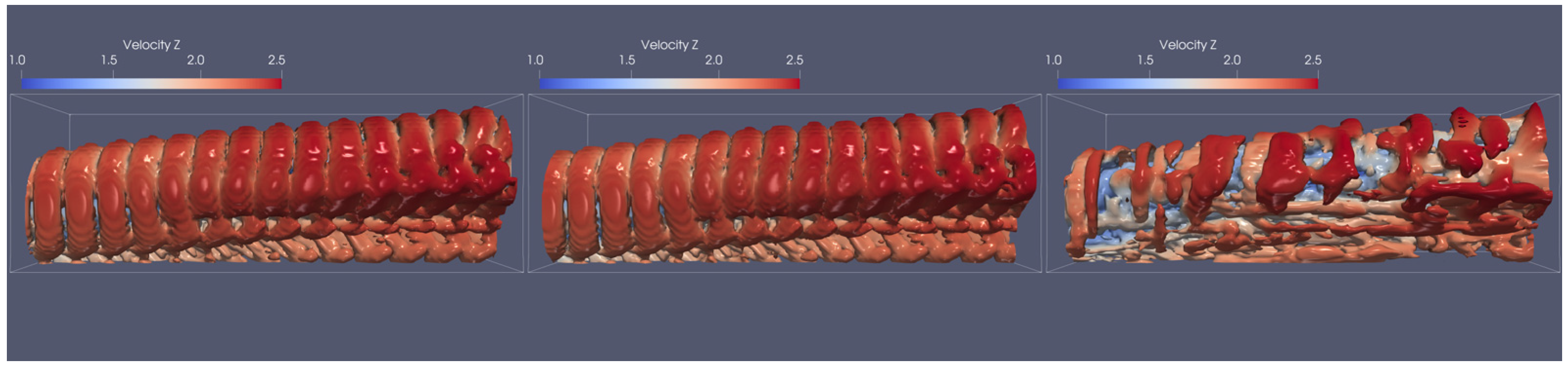
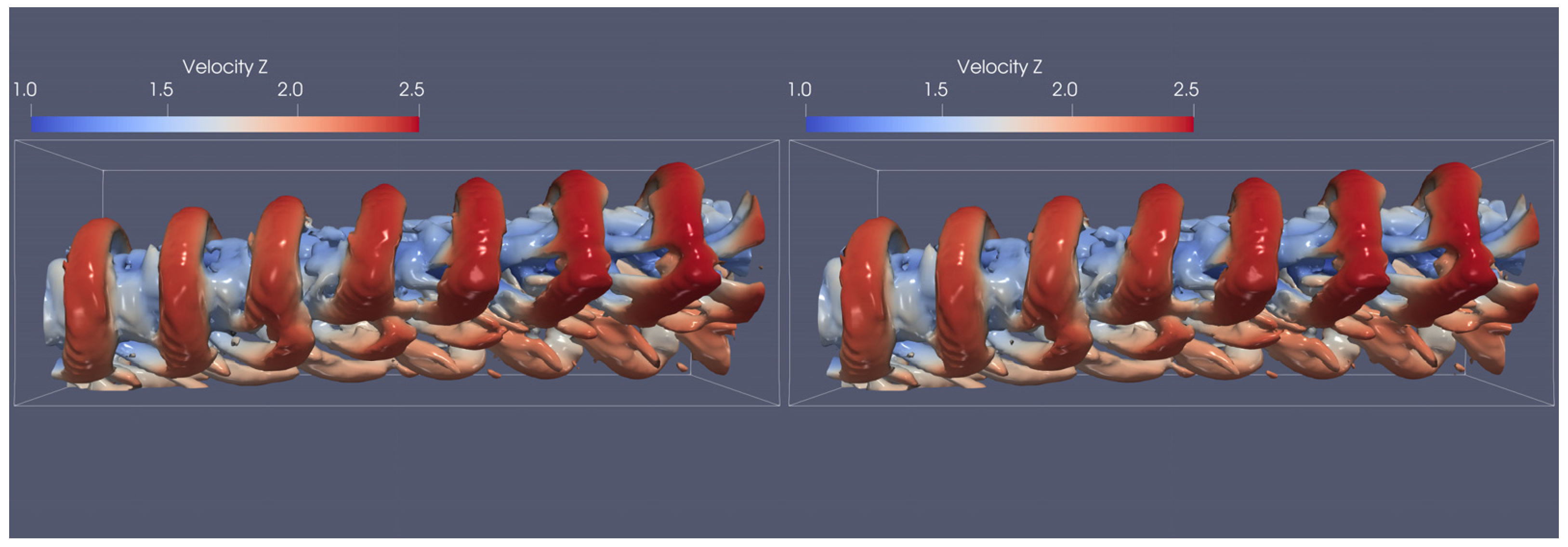
The additional normalization does not alter the topology of the modes. Figure 18, Figure 19, Figure 20 and Figure 21 present the vortex structures for Case 1 and Case 7 under min–max and standard normalization, respectively. Because the modal shapes in Cases 1–6 are nearly identical, only the vortex structures for Case 1 are shown for comparison. No noticeable changes in the vortex patterns are observed in any of the modes, further confirming that normalization has negligible influence on the modal topology.

3.3. NMF of Liutex

Figure 22 presents the first three spatial modes extracted from the same dataset using NMF. Because NMF requires all matrix entries to be non-negative, the decomposition is performed on the Liutex magnitude, R . In contrast to POD—which identifies energy-optimal spectral modes—NMF yields characteristic or parts-based modes that isolate physically interpretable structures. The first two NMF modes capture the conjugate ring-like vortices at different phases, while the third mode isolates the inner streamwise counter-rotating vortices.
This result is significant in several ways. First, it demonstrates that complex vortex systems can be decomposed into simpler, more localized components that are easier to interpret and manipulate. For instance, if one is interested in estimating the vortex core location, the outer ring-like structures can be excluded and only the inner vortices analyzed. Second, this characteristics-based decomposition may benefit downstream tasks such as vortex detection, clustering, or classification—analogous to how NMF is used in facial recognition to extract meaningful features rather than global patterns. Finally, with appropriate tuning of the sparsity constraint, NMF has the potential to reveal additional localized or intermittent flow structures that POD may overlook, particularly in more complex or multi-scale vortex environments.
Figure 23 presents the reconstructed vortex structures using 11 NMF modes (70% TKE preserved) at the same time instances examined in the POD analysis. The visualizations show no evidence of pseudo-vortices or other artificial features, and no significant loss of physical detail in the recovered flow field. This demonstrates that NMF is capable of preserving the essential vortex dynamics even when only a small number of dominant modes are retained. The corresponding MSE for the NMF reconstruction is 0.855993, and this value remains unchanged when additional normalization (rescaling) is applied. This further confirms that normalization has negligible influence on the reconstruction quality for NMF, and that the method remains robust in capturing the primary flow structures with a limited modal basis.

4. Discussion

This study evaluates the performance of two dimensionality reduction techniques—Proper Orthogonal Decomposition (POD) and Non-negative Matrix Factorization (NMF)—for analyzing complex vortex structures in high-speed turbulent boundary layers controlled by micro-vortex generators (MVGs). Using high-fidelity numerical simulations of Mach 2.5 flow, we examined how different flow variables and normalization strategies influence the interpretability, robustness, and reconstruction accuracy of the extracted coherent structures.
The results show that POD effectively captures the dominant energetic content of the flow. Across all cases involving velocity, only 3–4 modes are required to preserve 70% of the TKE, yielding reconstructions with MSE values on the order of 0.1. The case using Liutex components requires more modes (14 modes) to reach the same TKE threshold, yet it achieves a noticeably lower MSE (approximately 0.04). Overall, when the same number of modes is used, the reconstruction performance is comparable across all cases. The analysis also indicates that POD performance is strongly influenced by the choice of input variables: velocity- and Liutex-based inputs produce smoother and more physically coherent spatial modes, whereas density- and momentum-based inputs introduce additional small-scale variations that reduce interpretability. Normalization strategies, including min–max scaling and standard rescaling, exert only a minor influence on the resulting modes, suggesting that the intrinsic physical characteristics of the variables themselves primarily determine the quality of the POD.
In contrast, NMF provides a parts-based, non-orthogonal representation that enhances physical interpretability. Although it shows relatively higher MSE in reconstruction (about 0.8 in the case presented), NMF successfully isolates localized flow features, such as outer ring-like vortices and inner streamwise vortices, without producing the pseudo-structures that often appear in truncated POD reconstructions. This makes NMF particularly valuable for flows with multiple interacting vortex systems, where identifying distinct physical mechanisms is essential.
It is also important to note that the numerical simulations used in this study are fully dimensionless, and the vortex structures present in the dataset are sufficiently complex to be representative of a broad class of fluid dynamics environments. As a result, the methods and insights developed here are not limited to the specific supersonic MVG-controlled boundary layer examined. The Liutex-based decomposition framework, together with POD and NMF, can be readily applied to a wide range of hydraulic and environmental flow systems where complex vortex interactions govern the underlying physics. Because the simulations in this study are fully dimensionless and the vortex structures represented in the dataset are sufficiently rich to mirror those found in many real-world flows, the methodology is not limited to the specific supersonic configuration examined here. This framework therefore provides a transferable toolset for analyzing, interpreting, and reconstructing coherent structures in diverse fluid dynamics environments, and it offers valuable guidance for data-driven flow prediction and reduced-order modeling across a broad spectrum of hydraulic applications.

5. Conclusions

This work demonstrates that integrating the Liutex vortex identification method with POD and NMF offers a rigorous and efficient framework for analyzing complex vortex dynamics in high-speed aerodynamic flows. POD remains a powerful tool for capturing dominant energetic structures, while NMF excels at extracting localized, physically meaningful components. Together with Liutex—which provides a mathematically precise measure of fluid rotation—these techniques form a robust foundation for future developments in vortex recognition, clustering, and reduced-order modeling. Overall, the integrated use of Liutex, POD, and NMF establishes a robust foundation for future work in vortex identification, clustering, and reduced-order modeling. The framework developed here is broadly applicable to vortex-dominated flows beyond the specific supersonic case studied, offering a powerful toolset for advancing data-driven analysis in complex aerodynamic environments.

Author Contributions

Conceptualization and methodology, Y.Y. (Yonghua Yan); formal analysis, M.A.S., J.T., A.P., L.D. and S.P.; writing—original draft preparation, M.A.S., J.T., A.P., L.D., S.P. and C.C.; writing—review and editing, M.A.S., J.T., A.P., L.D., S.P., C.C. and Y.Y. (Yong Yang); visualization, M.A.S., J.T., A.P. and L.D. All authors have read and agreed to the published version of the manuscript.

Funding

This research is supported by the Mississippi NASA EPSCoR program and the R.I.S.E. Together Title III Mini Grant Program of Jackson State University.

Data Availability Statement

Data is contained within the article.

Acknowledgments

This work relied on computations performed on the WTAMU HPC cluster, which was funded by the National Science Foundation (NSF CC* GROWTH 2018841).

Conflicts of Interest

The authors declare no conflicts of interest.

Nomenclature

CFDComputational fluid dynamics
MVGMicro-vortex generator
PCAPrincipal component analysis
PODProper orthogonal decomposition
NMFNon-negative matrix factorization
TKETurbulence kinetic energy
ETotal energy
ρDensity
pPressure
x, y, zSpanwise, normal, and streamwise coordinate axes
u, v, wSpanwise, normal, and streamwise velocity
L X ,   L Y ,   L Z Spanwise, normal, and streamwise Liutex components

References

  1. Moffatt, H.K.; Shuckburgh, E. (Eds.) Environmental Hazards: The Fluid Dynamics and Geophysics of Extreme Events; World Scientific Publishing Co., Pte. Ltd.: Singapore, 2011. [Google Scholar]
  2. Jiang, X.; Lefauve, A.; Dalziel, S.B.; Linden, P.F. The evolution of coherent vortical structures in increasingly turbulent stratified shear layers. J. Fluid Mech. 2022, 947, A30. [Google Scholar] [CrossRef]
  3. Weiss, J. A Tutorial on the Proper Orthogonal Decomposition. In Proceedings of the 2019 AIAA Aviation Forum, Dallas, TX, USA, 17–21 June 2019. [Google Scholar]
  4. Gu, X.; Xu, C.; Liu, M.; Mao, Y. Frequency-domain proper orthogonal decomposition for efficient reconstruction of unsteady flows. Phys. Fluids 2025, 37, 025161. [Google Scholar] [CrossRef]
  5. Rowley, C.W. Model Reduction for Fluids, Using Balanced Proper Orthogonal Decomposition. Int. J. Bifurc. Chaos 2005, 15, 997–1013. [Google Scholar] [CrossRef]
  6. Bui-Thanh, T.; Willcox, K. Model Reduction for Large-Scale CFD Applications Using Balanced POD. In Proceedings of the 17th AIAA Computational Fluid Dynamics Conference, Toronto, ON, Canada, 6–9 June 2005. [Google Scholar]
  7. Taira, K.; Brunton, S.L.; Dawson, S.T.; Rowley, C.W.; Colonius, T.; McKeon, B.J.; Schmidt, O.T.; Gordeyev, S.; Theofilis, V.; Ukeiley, L.S. Modal Analysis of Fluid Flows: An Overview. AIAA J. 2017, 55, 4013–4041. [Google Scholar] [CrossRef]
  8. Zhang, Z.; Qin, Z.-J.; Huo, J.; Zhang, Y.; Liu, Q.-K. Physics-informed dynamic mode decomposition for reconstruction and prediction of dense particulate pipe flows. Phys. Fluids 2024, 36, 113374. [Google Scholar] [CrossRef]
  9. Minh, H.; Nguyen, F.T. Robust Kernel Principal Component Analysis. In Proceedings of the Advances in Neural Information Processing Systems, Vancouver and Whistler, BC, Canada, 8–13 December 2008. [Google Scholar]
  10. Solera-Rico, A.; Sanmiguel Vila, C.; Gómez-López, M.; Wang, Y.; Almashjary, A.; Dawson, S.T.M.; Vinuesa, R. β-Variational autoencoders and transformers for reduced-order modelling of fluid flows. Nat. Commun. 2024, 15, 1361. [Google Scholar] [CrossRef] [PubMed]
  11. Li, R.; Song, S. Manifold learning-based reduced-order model for full speed flow field. Phys. Fluids 2024, 36, 087117. [Google Scholar] [CrossRef]
  12. Babinsky, H.; Li, Y.; Pitt Ford, C.W. Microramp Control of Supersonic Oblique Shock-Wave/Boundary-Layer Interactions. AIAA J. 2009, 47, 668–675. [Google Scholar] [CrossRef]
  13. Nishantt, N.; Baraiya, N.A. Analysis of four wall flow control in supersonic duct using ramped-vanes micro vortex generator. CEAS Aeronaut. J. 2024, 15, 191–205. [Google Scholar] [CrossRef]
  14. Liu, J.; Khine, Y.Y.; Saleem, M.; Lopez Rodriguez, O.; Gutmark, E. Supersonic Jet Noise Reduction Using Micro Vortex Generators. In Proceedings of the AIAA AVIATION 2021 FORUM, Virtual, 2–6 August 2021. [Google Scholar]
  15. Yan, Y.; Chen, L.; Li, Q.; Liu, C. Numerical Study of Micro-Ramp Vortex Generator for Supersonic Ramp Flow Control at Mach 2.5. Shock Waves 2017, 27, 79–96. [Google Scholar] [CrossRef]
  16. Chen, C.; Yang, Y.; Yan, Y. Computational Analysis of Tandem Micro-Vortex Generators for Supersonic Boundary Layer Flow Control. Computation 2025, 13, 101. [Google Scholar] [CrossRef]
  17. Yan, Y.; Yang, Y.; Chen, C.; Cotton, H.A.; Serrano, A. Numerical Study on the Ring-like Vortex Structure Generated by MVG in High-Speed Flows with Different Mach Numbers. Jpn. J. Indust. Appl. Math. 2022, 39, 3–18. [Google Scholar] [CrossRef]
  18. Lee, D.; Seung, S. Learning the parts of objects by non-negative matrix factorization. Nature 1999, 401, 788–791. [Google Scholar] [CrossRef] [PubMed]
  19. Lee, D.; Seung, H.S. Algorithms for Non-negative Matrix Factorization. Adv. Neural Inf. Process. Syst. 2001, 13, 556–562. [Google Scholar]
  20. Ren, B.; Pueyo, L.; Chen, C.; Choquet, E.; Debes, J.H.; Duechene, G.; Menard, F.; Perrin, M.D. Using Data Imputation for Signal Separation in High Contrast Imaging. Astrophys. J. 2020, 892, 74. [Google Scholar] [CrossRef]
  21. Subramani, K.; Smaragdis, P.; Higuchi, T.; Souden, M. Rethinking Non-Negative Matrix Factorization with Implicit Neural Representations. In Proceedings of the 2025 IEEE Workshop on Applications of Signal Processing to Audio and Acoustics (WASPAA), Tahoe City, CA, USA, 12–15 October 2025; pp. 1–5. [Google Scholar] [CrossRef]
  22. Guo, Y.; Holy, T.E. Recovering missing features in nonnegative matrix factorization via generalized singular value decomposition. iScience 2026, 29, 114708. [Google Scholar] [CrossRef] [PubMed]
  23. Liu, C.; Gao, Y.; Tian, S.; Dong, X. Rortex—A New Vortex Vector Definition and Vorticity Tensor and Vector Decompositions. Phys. Fluids 2018, 30, 035103. [Google Scholar] [CrossRef]
  24. Alvarez, O. What Is Liutex? In Proceedings of the Vortex Workshop. VW 2023; Springer Proceedings in Physics; Wang, Y., Liu, C., Li, Y., Eds.; Springer: Singapore, 2024. [Google Scholar] [CrossRef]
  25. Yu, Y.; Alvarez, O.; Liu, C. Objective Liutex from Flow Data Measured in a Non-Inertial Frame. Fluids 2025, 11, 4. [Google Scholar] [CrossRef]
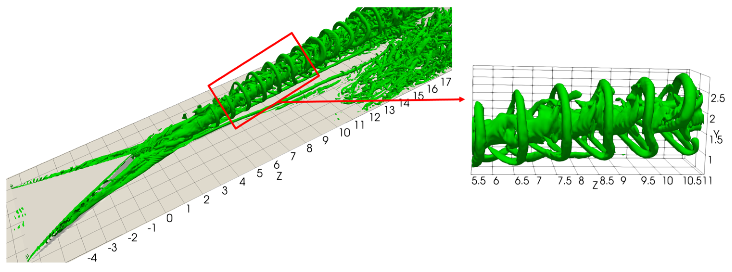
Figure 1. Vortex structure from the previous numerical simulation.
Computation 14 00122 g001
Figure 2. Illustration of the flow data preparation.
Computation 14 00122 g002
Figure 3. The first three dominant spatial modes contributing to TKE from Case 1, using POD with ( u , v , w ).
Computation 14 00122 g003
Figure 4. The first three dominant spatial modes contributing to TKE from Case 2, using POD with ( u , v , w , E).
Computation 14 00122 g004
Figure 5. The first three dominant spatial modes contributing to TKE from Case 3, using POD with ( ρ ,   u   ,   v ,   w ).
Computation 14 00122 g005
Figure 6. The first three dominant spatial modes contributing to TKE from Case 4, using POD with ( ρ ,   u   ,   v ,   w , E).
Computation 14 00122 g006
Figure 7. The first three dominant spatial modes contributing to TKE from Case 5, using POD with ( ρ u ,   ρ v ,   ρ w ).
Computation 14 00122 g007
Figure 8. The first three dominant spatial modes contributing to TKE from Case 6, using POD with ( ρ u ,   ρ v ,   ρ w , E).
Computation 14 00122 g008
Figure 9. The first three dominant spatial modes contributing to TKE from Case 7, using POD with ( L X ,   L Y ,   L Z ).
Computation 14 00122 g009
Figure 10. Vortex structure from the original simulation data at timesteps 199,900 (left) and 200,000 (right).
Computation 14 00122 g010
Figure 11. Reconstruction of the vortex structure from Case 1 ( u , v , w ) at timesteps 199,900 (left) and 200,000 (right).
Computation 14 00122 g011
Figure 12. Reconstruction of the vortex structure from Case 2 ( u , v , w , E) at timesteps 199,900 (left) and 200,000 (right).
Computation 14 00122 g012
Figure 13. Reconstruction of the vortex structure from Case 3 ( ρ ,   u ,   v ,   w ) at timesteps 199,900 (left) and 200,000 (right).
Computation 14 00122 g013
Figure 14. Reconstruction of the vortex structure from Case 4 ( ρ ,   u ,   v ,   w , E) at timesteps 199,900 (left) and 200,000 (right).
Computation 14 00122 g014
Figure 15. Reconstruction of the vortex structure from Case 5 ( ρ u ,   ρ v ,   ρ w ) at timesteps 199,900 (left) and 200,000 (right).
Computation 14 00122 g015
Figure 16. Reconstruction of the vortex structure from Case 6 ( ρ u ,   ρ v ,   ρ w ,   E ) at timesteps 199,900 (left) and 200,000 (right).
Computation 14 00122 g016
Figure 17. Reconstruction of the vortex structure from Case 7 ( L X ,   L Y ,   L Z ) at timesteps 199,900 (left) and 200,000 (right).
Computation 14 00122 g017
Figure 18. The first three dominant spatial modes contributing to TKE from Case 1, using POD with ( u , v , w ) and min-max normalization.
Computation 14 00122 g018
Figure 19. The first three dominant spatial modes contributing to TKE from Case 7, using POD with ( L X ,   L Y ,   L Z ) and min-max normalization.
Computation 14 00122 g019
Figure 20. The first three dominant spatial modes contributing to TKE from Case 1, using POD with ( u , v , w ) and standard rescaling.
Computation 14 00122 g020
Figure 21. The first three dominant spatial modes contributing to TKE from Case 7, using POD with ( L X ,   L Y ,   L Z ) and standard rescaling.
Computation 14 00122 g021
Figure 22. The first three spatial modes using NMF with |L|.
Computation 14 00122 g022
Figure 23. Reconstruction of the Liutex magnitude field at timesteps 199,900 (left) and 200,000 (right), using NMF with |L|.
Computation 14 00122 g023
Table 1. Cases with different variables used in the POD/PCA.
CaseVariables UsedModes Required for 70% TKEMSE (70% TKE)MSE (14 Modes)
1 u , v , w 40.100.05
2 u , v , w , E40.120.05
3 ρ ,   u   ,   v ,   w 30.100.05
4 ρ ,   u   ,   v ,   w , E30.100.05
5 ρ u ,   ρ v ,   ρ w 30.110.05
6 ρ u ,   ρ v ,   ρ w , E30.110.05
7 L X ,   L Y ,   L Z 140.040.04
Table 2. Number of modes required for 70% TKE and the MSE for each case with min-max normalization method.
CaseVariables UsedModes Required for 70% TKEMSE (70% TKE)MSE (14 Modes)
1 u , v , w 40.100.05
2 u , v , w , E40.120.05
3 ρ ,   u ,   v ,   w 30.100.05
4 ρ ,   u ,   v ,   w , E30.100.05
5 ρ u ,   ρ v ,   ρ w 30.110.05
6 ρ u ,   ρ v ,   ρ w , E30.110.05
7 L X ,   L Y ,   L Z 140.050.05
Table 3. Number of modes required for 70% TKE and the MSE for each case with standard rescaling method.
CaseVariables UsedModes Required for 70% TKEMSE (70% TKE)MSE (14 Modes)
1 u , v , w 40.100.05
2 u , v , w , E40.120.05
3 ρ ,   u ,   v ,   w 30.100.05
4 ρ ,   u ,   v ,   w , E30.100.05
5 ρ u ,   ρ v ,   ρ w 30.110.05
6 ρ u ,   ρ v ,   ρ w , E30.110.05
7 L X ,   L Y ,   L Z 140.040.04
Disclaimer/Publisher’s Note: The statements, opinions and data contained in all publications are solely those of the individual author(s) and contributor(s) and not of MDPI and/or the editor(s). MDPI and/or the editor(s) disclaim responsibility for any injury to people or property resulting from any ideas, methods, instructions or products referred to in the content.