Computational Assessment of Shear Stress-Driven Flow Alterations at the Renal Artery Origin Under Varying Pressure Conditions

Abstract

The use of computational fluid dynamics (CFD) to study hemodynamics in arteries offers significant potential for addressing complex flow problems. Due to its enhanced performance hardware and software, CFD has become an important approach for studying hemodynamics in human arteries. This approach is utilized to investigate hemodynamics and forecast risk factors for atherosclerotic lesion development and progression, including circulatory flow, and to analyze local flow fields and flow profiles resulting from geometric changes. This foundational study will aid in analyzing blood flow behavior through the abdominal aorta and the origin and courses of renal arteries, as well as investigating the causes of disorders such as atherosclerosis and hypertension. The current study investigates three idealized abdominal aorta–renal artery junction models under varying blood pressure settings. Materialise software V19 was used to extract the geometry data to create idealized 3D abdominal aorta–renal branching models. Unsteady flow simulations were performed in ANSYS Fluent, utilizing rigid walls and Newtonian and Carreau–Yasuda viscosity conditions. Oscillatory shear index (OSI) and Time-averaged wall shear stress (TAWSS) were measured to enhance understanding of atherosclerotic plaque formation and progression. Also, the effect of geometric change at the bifurcation area was explored, and it was discovered that this location causes considerable vortex forming zones. The evident velocity reduction and backflow development were seen, reducing shear stress. The findings indicate that low TAWSS < 0.4 Pa and OSI > 0.15 areas within the bifurcation region are more susceptible to atherosclerosis development.

1. Introduction

Recent advances in computation have expanded the scope of multidisciplinary research in the biomedical engineering discipline. Numerical simulations are increasingly used to understand complex physiological phenomena, support clinicians in decision-making, and complement existing diagnostic modalities. In cardiovascular research, Computational Fluid Dynamics (CFD) and Fluid–Structure Interaction (FSI) modeling aids the improved visualization of conditions and quantification of hemodynamic parameters such as blood velocity, pressure distribution, and wall shear stress (WSS). While FSI offers the highest level of physiological realism by accounting for wall deformations, rigid-wall CFD remains a critical and validated tool for quantifying intraluminal shear metrics, especially when the focus is on the impact of severe geometric constrictions. This provides insights into vascular pathophysiology that are difficult to obtain through non-invasive measurements. CFD has thus emerged as a valuable non-invasive tool for evaluating the flow mechanics within the arteries, enhancing the understanding of blood flow behavior in both healthy and diseased states [1,2,3,4].

Renal artery stenosis (RAS), a blockage in the artery, often resulting from atherosclerotic plaque build-up in the intimal vessel wall [5,6,7,8,9]. This is a major cause of secondary hypertension and thereby renal dysfunction and other conditions. The constricted renal arteries restrict the perfusion, thereby activating the renin–angiotensin–aldosterone system (RAAS) and leading to increased systemic blood pressure, which is generally identified as a symptom of drug-resistant hypertension [8,9]. While in normal physiological conditions, the kidneys receive approximately 20–25% of cardiac output [10]. The reduction in the renal blood supply resulting from stenosis disrupts this balance and can result in hypertensive complications. While anatomical imaging techniques such as digital subtraction angiography (DSA), duplex ultrasound, magnetic resonance angiography (MRA), and computed tomographic angiography (CTA) are commonly used modalities to detect RAS, they provide limited functional information about hemodynamic impact and plaque progression [11,12].

The geometry of the vasculature also plays a pivotal role in determining local flow characteristics [13,14]. Arterial bifurcations and curved regions, like the renal artery branching from the abdominal aorta, are susceptible to complex flow patterns, such as flow separation and recirculation [15,16,17]. These disturbed flow patterns are closely linked to changes in shear stress; regions with continuously low WSS and high oscillatory shear index (OSI) correlate with endothelial dysfunction and lipid accumulation, while high, unidirectional shear tends to confer protective effects against atherogenesis [18,19]. Vascular research continues to emphasize the association between hemodynamic forces and vascular disease progression. This reinforces the fact that shear-related metrics derived from CFD are critical indicators of lesion-prone regions and their assessment for risk [20,21].

Even though there is an upward surge in the usage of CFD in cardiovascular research, most of the studies remain concentrated on normal blood pressure conditions and do not systematically explore the hemodynamic effects of physiological variability, such as hypertensive or hypotensive states or dynamically varying blood pressure. Systemic blood pressure mainly changes the flow dynamics, influencing velocity, pressure gradients, and shear stress distributions. This can impair the disease progression, depending on the underlying vascular geometry [22,23,24]. Additionally, while blood exhibits non-Newtonian rheological behavior, many CFD studies assume Newtonian flow for simplicity; the impact of non-Newtonian modeling, particularly in stenosed arteries, continues to be investigated to capture realistic shear-thinning effects [25,26,27].

The abdominal aorta and its renal branches pose a distinctive interest in hemodynamics due to their anatomical orientation and branching angles [28,29]. Variations in branching geometry can significantly alter hemodynamic forces such as WSS, pressure gradients, and flow separation, finally influencing the localization and development of atherosclerotic plaques [30,31,32]. Bifurcation zones with low WSS and high OSI are particularly susceptible to plaque accumulation, while high shear regions are atheroprotective [33,34,35].

This study considers CFD to systematically investigate pulsatile blood flow in idealized abdominal aorta–renal artery models under healthy, single stenosed, and double stenosed configurations, with additional comparisons across systemic pressure variations and various viscosity models. By examining velocity distribution, pressure gradients, wall shear stress, time-average wall shear stress (TAWSS), and OSI, the present work aims to explain how geometric obstruction, blood pressure, and viscosity collectively influence arterial hemodynamics and thereby disease progression. The findings are expected to contribute a flow dynamic point of view into RAS, and these insights shall support the growing role of computational modeling in clinical evaluation.

2. Materials and Methods

2.1. Governing Equations

The hemodynamic investigation in the abdominal aorta–renal artery system assumes blood flow to be incompressible and laminar within the computational domain. The laminar flow regime was verified by calculating the peak Reynolds number at the renal branch. In the stenosed renal arteries, the Reynolds number varies in the range of Re~290–317 depending on the local cross-section. This is lower than the value observed in the healthy renal artery (Re~789). This reduction occurs because the decrease in artery diameter, together with the significant reduction in flow rate, outweighs the relatively small increase in velocity within the stenosed region. The Womersley numbers within the stenosis are less than 1. To evaluate the influence of rheological modeling, blood is modeled both as a Newtonian fluid and as a non-Newtonian fluid using the Carreau–Yasuda model.

The governing equations used are the continuity and the incompressible Navier–Stokes equation [36,37] shown in Equations (1) and (2).

$$\nabla .\overrightarrow{v}=0$$

(1)

$$\rho \left({\displaystyle \frac{\partial \overrightarrow{v}}{\partial t}}+\overrightarrow{v}.\mathsf{\nabla }\overrightarrow{v}\right)=\mathsf{\nabla }p+\nabla .\stackrel{̿}{\mathrm{\tau }}$$

(2)

$$\stackrel{̿}{\mathrm{\tau }}=\eta (\dot{\gamma })[\nabla .\overrightarrow{v}{+(\nabla .\overrightarrow{v})}^{\mathrm{T}}]$$

(3)

where $\overrightarrow{v}$ is the velocity vector, $\rho$ is the density, $p$ is the pressure, $\stackrel{̿}{\mathrm{\tau }}$ is the viscous stress tensor and $\dot{\gamma }$ is the shear rate, and $\eta$ is the blood viscosity. The body force/gravity term is not considered.

Viscosity represents the resistance a fluid offers to deformation or flow. Under Newtonian assumptions, viscosity maintains a linear relationship with shear rate [16,37]. However, in non-Newtonian fluids, shear stress does not vary linearly with the rate of shear strain. One important characteristic of such fluids is shear-thinning behavior, in which viscosity decreases as the shear rate increases. Blood exhibits this shear-thinning nature particularly at lower shear rates, typically below 100 s⁻¹ [32]. Carreau–Yasuda fluid model [38,39,40] accounts for the shear-thinning property in Equation (4)

$$\mathrm{\eta }\left(\dot{\gamma }\right)={\mathrm{\eta }}_{\mathrm{\infty }}+\left({\mathrm{\eta }}_0-{\mathrm{\eta }}_{\mathrm{\infty }}\right){\left[1+{\left(\mathrm{\lambda }\dot{\gamma }\right)}^{\mathrm{a}}\right]}^{{\displaystyle \frac{\mathrm{n}-1}{\mathrm{a}}}}$$

(4)

Equation (4) is a generalization of the Newtonian model and describes the variation in viscosity $\mathrm{\eta }$ with shear rate $\dot{\gamma }$ than other rheological models. The fundamental characteristic of this formulation is that the Carreau–Yasuda equation involves five parameters as described in

Table 1. Parameter table for Carreau–Yasuda model [32].

Parameter	Symbol	Value	Unit
Zero-shear Viscosity	${\eta }_0$	0.022	Pa.s
Infinite-shear Viscosity	${\eta }_{\mathrm{\infty }}$	0.0022	Pa.s
Relaxation Time	$\mathrm{\lambda }$	0.11	s
Power-law Index	$\mathrm{n}$	0.392	Dimensionless
Yasuda Exponent	$\mathrm{a}$	0.644	Dimensionless

[32], whereas for the Newtonian fluid considerations, the constant blood viscosity $\eta$ of 0.00345 Pa.s and density of 1050 kg/m³ were adopted.

Hemodynamic descriptors Time-Averaged Wall Shear Stress (TAWSS) determines the average magnitude of the shear stress vector over a full cardiac cycle pulse T given in Equation (5) [38,41,42].

$$TAWSS={\displaystyle \frac{1}{T}}{\int }_0^T\left|WSS\right|dt$$

(5)

Oscillatory Shear Index (OSI) quantifies the deviation of the wall shear stress from its main axial direction, identifying regions of flow reversal given in Equation (6).

$$\mathrm{O}\mathrm{S}\mathrm{I}=0.5\left(1-{\displaystyle \frac{\left|{\int }_0^{\mathrm{T}}\mathrm{W}\mathrm{S}\mathrm{S} \mathrm{d}\mathrm{t}\right|}{{\int }_0^{\mathrm{T}}\left|\mathrm{W}\mathrm{S}\mathrm{S}\right|\mathrm{d}\mathrm{t}}}\right)$$

(6)

2.2. Geometry Modeling

The computational domain represents an idealized abdominal aorta–renal artery bifurcation geometry obtained from the CT imaging and literature measurements. Anonymized CT-DICOM datasets obtained as part of an ongoing retrospective study (approved by the institutional ethics committee) were used to identify representative geometric features such as renal artery angulation, branch orientation, and characteristic vessel dimensions.

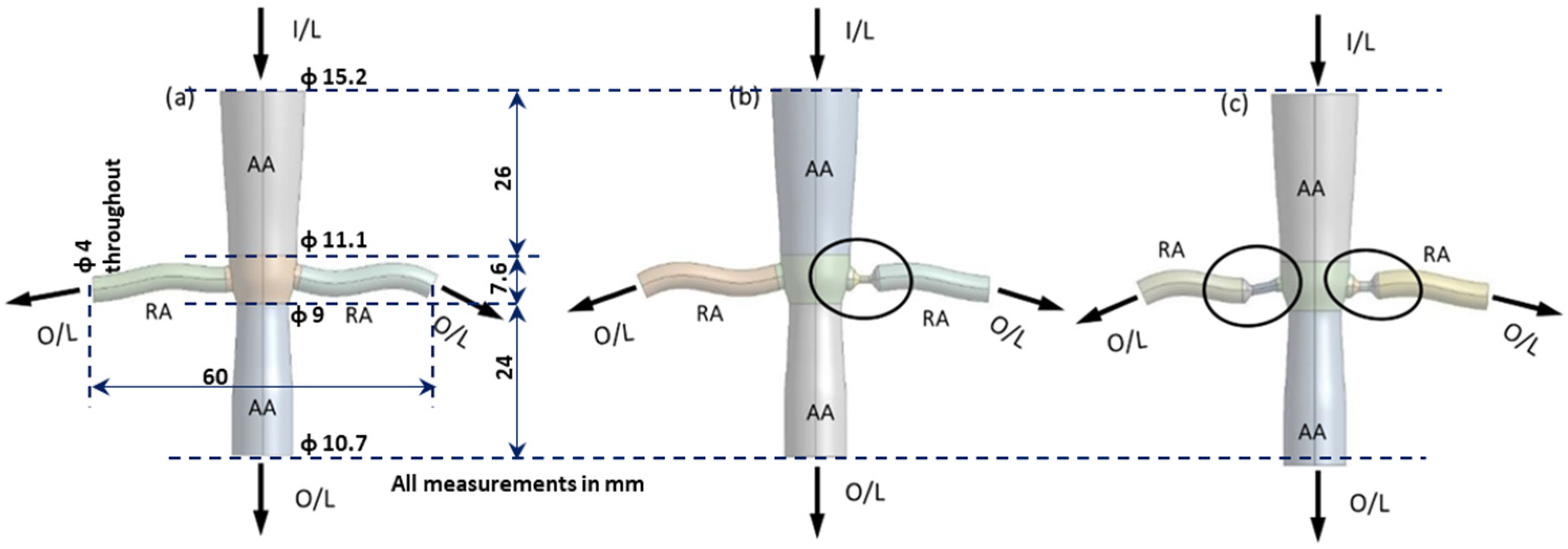
Geometric consistency was maintained, and systematic hemodynamic analysis was facilitated by simplifying the reconstructed anatomy into an idealized configuration using CAD processing tools [43,44]. The abdominal aorta segment was modeled as a straight cylindrical tube with a circular cross-section with a gradual taper in the downstream direction; cross-sectional and plane references are given in Figure 1a. The renal arteries were modeled as curved branches originating from the aortic wall with angulation consistent with anatomical measurements. The procedure for reconstruction was adopted from the literature [44,45,46]. Branch diameters and orientation were selected to represent typical renal artery geometry. Thus, the final geometry preserves the major anatomical characteristics influencing renal hemodynamics while eliminating patient-specific irregularities that could mask the general hemodynamic trends. The abdominal aorta was modeled as a tapered cylinder with a diameter varying from 15.2 mm to 10.7 mm at various planar sections, as shown in Figure 1a. Two asymmetric renal arteries of 4.0 mm diameter were modeled with 80° angulation with respect to the centerline of the abdominal aorta.

Renal artery stenosis was modeled as a localized concentric narrowing of the vessel lumen along the renal artery centerline. The stenotic region was constructed by reducing the vessel diameter over a segment while maintaining smooth transitions from proximal to distal regions. The geometry characteristics of stenosis were influenced by renal artery stenosis studies [28,45]. In this representation, the lumen reduction was assumed axisymmetric, with the maximum diameter reduction occurring at the center of the stenotic segment. The stenosis severity, defined as the percentage reduction in lumen diameter relative to the healthy vessel diameter, together with the axial length of the stenotic region and its location from the renal ostium, were specified as geometric parameters of the model in

Table 2. Stenosis model parameters.

Parameters	Unilateral Single Stenosed Case	Bilateral Double Stenosed Case
Healthy Renal Artery Diameter	4 mm	4 mm
Stenosis Severity (%)	72.5% diameter reduction in RRA	72.5% diameter reduction in RRA 65% diameter reduction in LRA
Stenosis Length	5.11 mm in RRA	5.11 mm in RRA 6.65 mm in LRA
Minimum Diameter	1.1 mm in RRA	1.1 mm in RRA 1.4 mm in LRA
Stenosis center distance from ostia	5.53 mm from right ostium	5.53 mm from right ostium 6.72 mm from left ostium

to facilitate reproducibility.

Three distinct geometric configurations were considered in this study: (i) Healthy, with no stenotic constrictions, henceforth named as Healthy case as shown in Figure 1a; (ii) Unilaterally stenosed, with a constriction in the right renal artery, henceforth called as Single Stenosed Case as shown in Figure 1b; and (iii) Bilaterally stenosed, with constrictions of various degrees in both renal arteries, henceforth called as double stenosed as shown in Figure 1c. Constrictions were introduced concentrically along the centerline of each renal branch without altering the parent aortic geometry. In the unilateral and bilateral stenosis configurations, concentric constrictions were introduced in the renal arteries. The reference diameter of both renal branches was 4 mm. For the right renal artery (RRA), the diameter was gradually reduced to a minimum of 1.1 mm over a stenosis length of 5.11 mm, corresponding to a 72.5% diameter reduction (92.4% area reduction), representing a severe stenotic condition. For the left renal artery (LRA), the minimum diameter was 1.4 mm over a stenosis length of 6.65 mm, corresponding to a 65% diameter reduction (87.8% area reduction). Stenoses were created to mention minimum diameter with a gradual variation from the baseline diameter. Step wise profile was lofted to ensure continuity in the curvature. All vessel walls were assumed rigid, and inlet and outlet boundary surfaces were considered with circular cross-sectional faces normal to the flow direction. The centerline points used for hemodynamic evaluation were distributed along the flow direction from the suprarenal aortic inlet through the infrarenal region.

2.3. Meshing

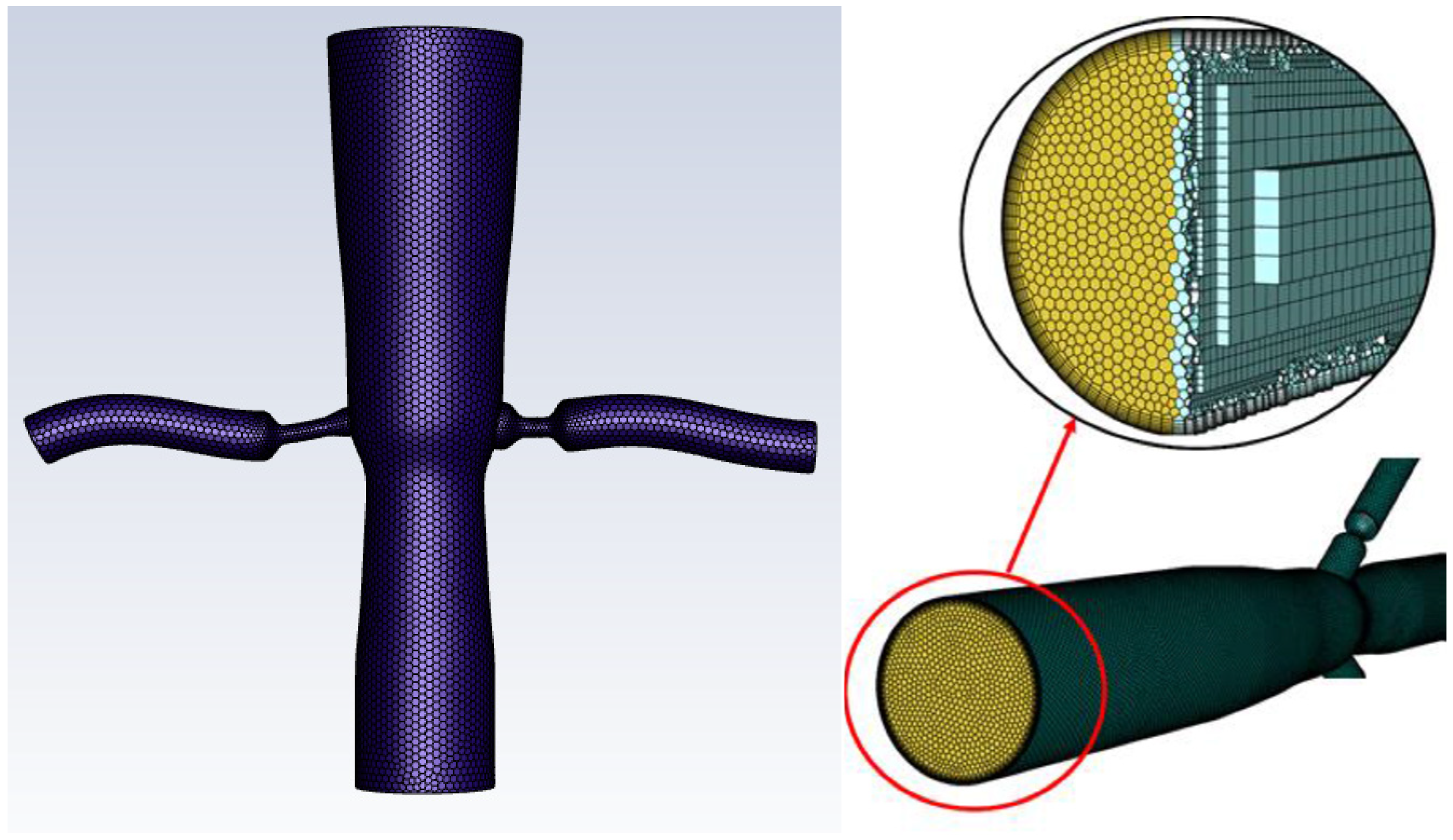
The computational domain was discretized using a poly-hexacore mesh [46], consisting of polyhedral elements in the near-wall and surface regions and structured hexahedral elements within the core, as shown in Figure 2. This hybrid approach was adopted to ensure improved numerical stability and reduced cell count while maintaining adequate resolution of complex flow features near geometric transitions. The surface mesh was created with a target element size ranging from 0.5 mm to 0.8 mm, with a growth rate of 1.2. The interior region was meshed with hexahedral elements of size 0.8 mm.

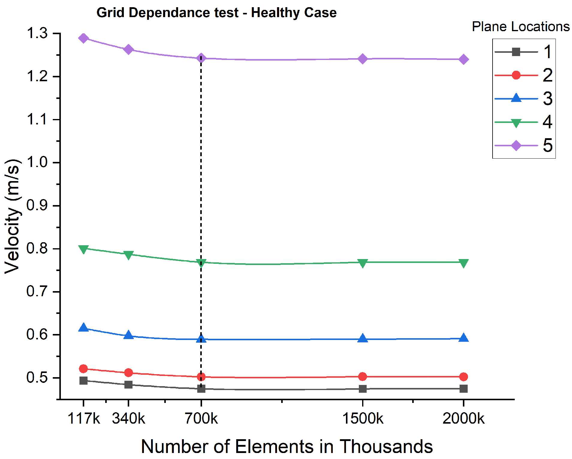
A grid independence study was conducted under steady-state conditions to check the sensitivity of mesh density on various parameters. Five consecutively refined meshes consisting of approximately 117 × 10³, 340 × 10³, 700 × 10³, 1500 × 10³, and 2000 × 10³ elements were examined. Key hemodynamic quantities, including velocity magnitude and wall pressure distribution, were monitored at mid-flow axial locations as shown in Figure 3. The results demonstrated tolerable variation (<2%) beyond the 700 × 10³ element mesh, indicating grid convergence. Accordingly, the mesh containing approximately 700,000 elements was selected for all subsequent simulations as an optimum. Five prism-based boundary layers were generated along the vessel walls with a growth rate of 1.2 to adequately resolve near-wall velocity gradients and accurately capture wall shear stress-linked quantities. The geometries with stenosis were also discretized using the same strategy to maintain methodological consistency. Additional local refinement was applied in the stenotic regions to ensure adequate spatial resolution of steep velocity gradients associated with flow. Consequently, the stenosed models contained a higher local element density in the constricted segments, allowing for the accurate capture of complex hemodynamics.

2.4. Boundary Conditions

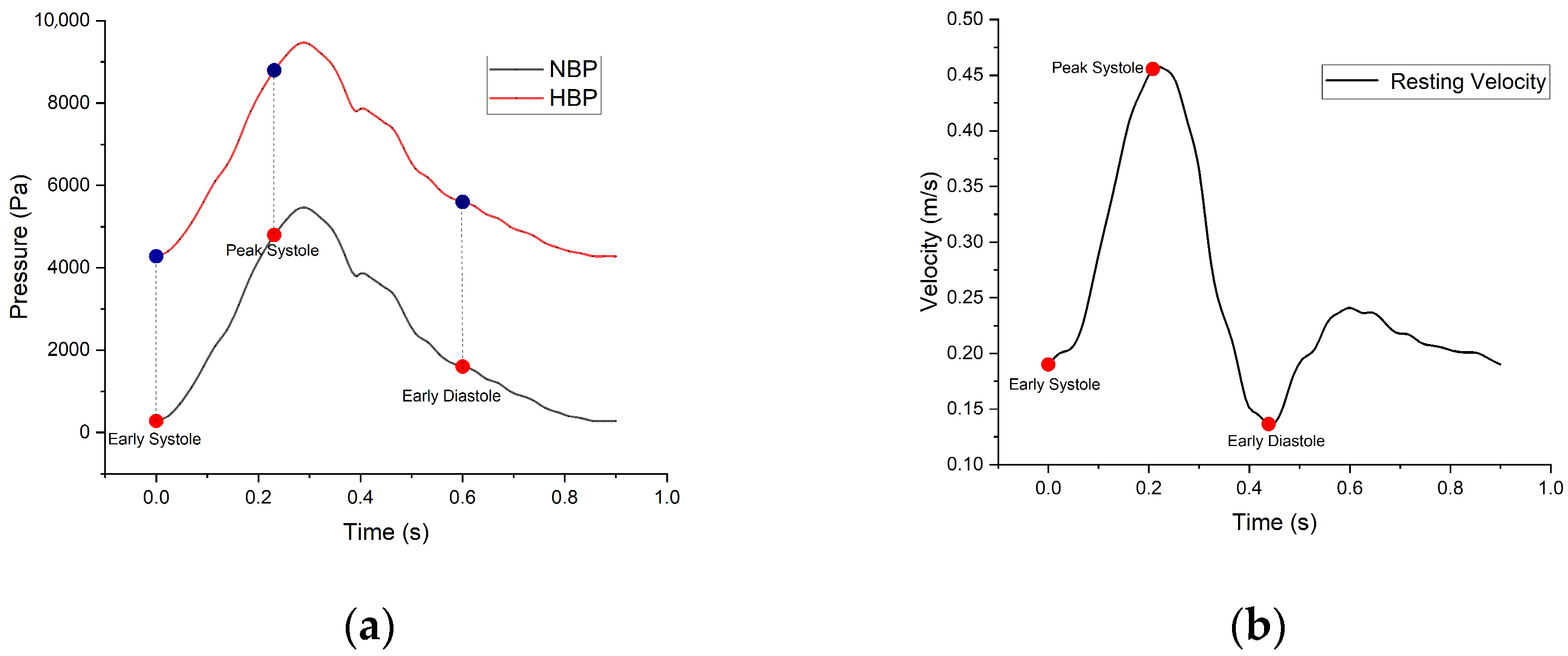
A time-dependent pulsatile velocity profile, as shown in Figure 4b, was defined at the inlet of the abdominal aorta using a user-defined function (UDF) [47,48]. The cardiac cycle duration was set to 0.9 s, representing physiological heart rate conditions [49,50]. At the outlets of the right and left renal arteries, as well as at the distal abdominal aorta pulsatile pressure boundary conditions were applied as shown in Figure 4a. Two physiological pressure conditions were considered: (i) normal blood pressure (80–120 mmHg) and (ii) high blood pressure (110–150 mmHg). Corresponding pulsatile renal outlet pressures were prescribed to maintain physiological pressure distribution across the branches. The inlet and outlet waveform was constructed in MATLAB R2024a by first generating representative physiological velocity/pressure data and subsequently fitting the waveform using a Fourier series expansion given in Equation (7) to ensure smooth periodic repetition across successive cardiac cycles [18]. The pulsatile inlet velocity and outlet pressure waveforms were reconstructed using an 8-term Fourier series representation given in Equation (7).

$$f(t)={\mathrm{a}}_0+{\sum }_{n=1}^8[{\mathrm{a}}_{\mathrm{n}}\mathrm{c}\mathrm{o}\mathrm{s} (\mathrm{n}\mathrm{\ast }\mathrm{t}\mathrm{\ast }\mathsf{\omega })+{\mathrm{b}}_{\mathrm{n}}\mathrm{s}\mathrm{i}\mathrm{n} (\mathrm{n}\mathrm{\ast }\mathrm{t}\mathrm{\ast }\mathsf{\omega }\left)\right]$$

(7)

where ω = 2π/T and T = 0.9 s is the cardiac cycle period. The Fourier coefficients used to reconstruct the velocity and pressure waveforms are provided in

Table 3. Fourier coefficients for pulsatile velocity and pressure.

Coefficient	Pulsatile Wave Form with 95% Confidence Bounds
	For Velocity	For Normal BP	For High BP
${\mathrm{a}}_0$	0.2534	2359	6358
${\mathrm{a}}_1$	0.01574	−1541	−1541
${\mathrm{b}}_1$	0.08219	1679	1679
${\mathrm{a}}_2$	−0.08768	−554.6	−554.6
${\mathrm{b}}_2$	0.01914	−415.3	−415.3
${\mathrm{a}}_3$	0.007292	54.92	54.92
${\mathrm{b}}_3$	−0.03692	−109.6	−109.6
${\mathrm{a}}_4$	0.002004	34.09	34.09
${\mathrm{b}}_4$	0.0000677	71.47	71.47
${\mathrm{a}}_5$	0.0003618	90.63	90.63
${\mathrm{b}}_5$	0.002163	52.55	52.55
${\mathrm{a}}_6$	0.0006391	41.99	41.99
${\mathrm{b}}_6$	−0.001551	11.34	11.34
${\mathrm{a}}_7$	0.002314	−53.39	−53.39
${\mathrm{b}}_7$	0.0001866	−26.25	−26.25
${\mathrm{a}}_8$	0.00162	31.16	31.16
${\mathrm{b}}_8$	0.001764	−22.88	−22.88
$\mathsf{\omega }$	6.954	7.018	7.018

to ensure full reproducibility of the boundary conditions.

This Fourier representation was then implemented within the CFD solver via a UDF to enforce temporally varying inlet and outlet conditions on the inlet and outlet faces of the domain [18,46]. A no-slip boundary condition is applied at the artery wall. The combination of pulsatile inlet velocity and outlet pressure conditions enabled a realistic simulation of transient hemodynamics under both normal blood pressure and high blood pressure states. In this foundational study, the arterial walls are considered to be rigid. This assumption is justified as the primary focus of the study is to compare the sensitivity of Newtonian vs. non-Newtonian models in the presence of unilateral and bilateral stenosis, where the flow physics inside the arteries are significant over small-scale wall displacements.

2.5. Solver Settings

CFD simulations were performed using ANSYS Fluent 2022 R2 with a pressure-based transient solver. The governing Navier–Stokes equations were solved using an implicit time integration scheme, and pressure–velocity coupling was achieved using the SIMPLE algorithm. Solutions were initialized from the inlet zone to promote stable convergence. A pulsatile cardiac cycle of 0.9 s was simulated for three consecutive cycles to ensure periodic flow development, and results were extracted from the final cycle to eliminate initial transient effects.

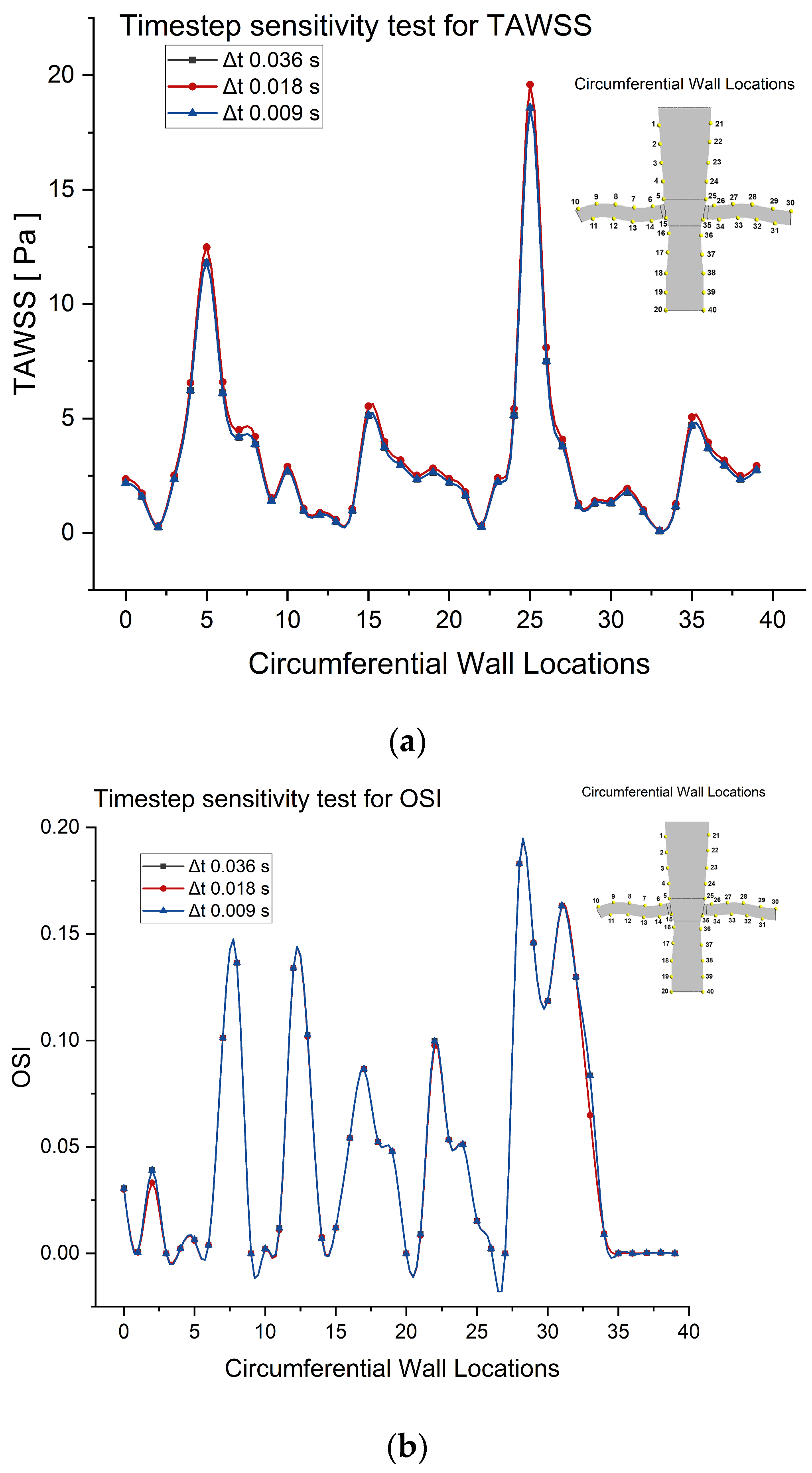
A timestep sensitivity analysis was performed to ensure that the temporal discretization does not influence the hemodynamic parameters. Each cardiac cycle was discretized into 25, 50, 100-timesteps in three iterations. Three different timestep sizes (0.036 s, 0.018 s, and 0.009 s) were evaluated, and the resulting variations in Oscillatory Shear Index (OSI) and Time-Averaged Wall Shear Stress (TAWSS) were examined at multiple circumferential wall locations as shown in Figure 5a,b. The results indicate that the differences between the smaller timesteps are minimal across all sampled points. In particular, the values obtained with 0.018 s and 0.009 s timesteps show very close agreement, suggesting that further reduction in timestep does not significantly alter the computed hemodynamic quantities. Based on this observation, the timestep of 0.018 s was considered sufficient to capture the transient flow behavior while maintaining computational efficiency. Within each time step, iterations were performed until residuals for continuity and momentum equations decreased below 10⁻⁶ or a maximum of 30 iterations was reached. Mass flow rate and pressure monitors at the inlet and outlets were employed to verify the global mass and flux balance within the simulation. The implicit formulation allowed stable time advancement without strict Courant number impositions in the simulations.

Spatial discretization of momentum equations was performed using second-order schemes to ensure improved solution accuracy, while temporal discretization employed a first-order implicit formulation to maintain numerical stability during transient pulsatile simulations. A comparison between first-order and second-order temporal discretization schemes was performed for the smallest timestep (0.009 s). The OSI and TAWSS results showed negligible differences, indicating that the solution is insensitive to the discretization scheme. Consequently, the first-order scheme was used in all simulations to reduce computational costs.

3. Results and Discussion

3.1. Velocity Contours

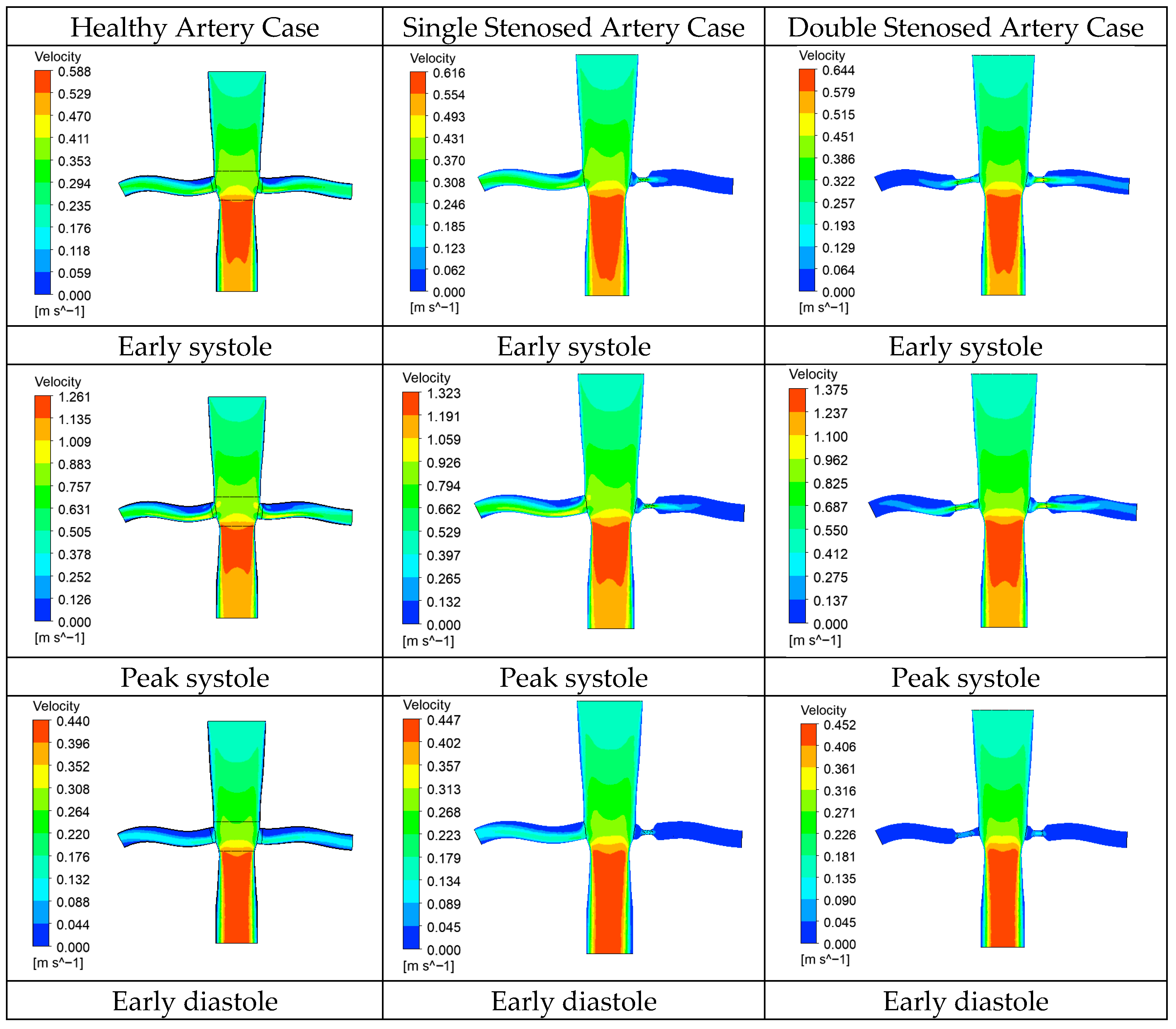
Figure 6 presents the velocity contours along the axial mid-plane of the abdominal aorta and renal branches for the healthy, single stenosed, and double stenosed geometries during early systole, peak systole, and early diastole, respectively.

During early systole, the velocity distribution remained relatively uniform in the healthy model, with smooth acceleration along the abdominal aorta and near symmetric flow division into the renal branches. The maximum velocities observed were 0.588 m/s (healthy), 0.614 m/s (single stenosis), and 0.644 m/s (double stenosis). In the stenosed models, flow acceleration was expected at the constriction throat, accompanied by the formation of localized high velocity regions. At peak systole, the differences became more prominent. Maximum velocities increased to 1.261 m/s, 1.323 m/s, and 1.375 m/s for the healthy, single stenosed, and double stenosed cases, respectively. In stenosed configurations, a strong jet formed at the stenosis throat, followed by a region of rapid deceleration downstream of the flow. Post-stenotic regions exhibited zones of reduced velocity adjacent to the wall, indicating flow separation and recirculation. These low-velocity regions were more widespread in the double stenosed model compared to the single stenosed case. During early diastole, overall peak velocities decreased to 0.44, 0.447, and 0.452 m/s. However, residual flow disturbances continued in the stenosed cases. The post-stenotic regions continued to show localized low-velocity pockets and asymmetric flow structures. The higher peak velocities observed in stenosed cases are consistent with stenotic jet formation as observed in previous studies [45,51], where flow contraction at the throat produces elevated local wall shear stresses.

Downstream of the stenosis, a rapid increase in the lumen cross-section leads to adverse pressure gradients, leading to flow separation and recirculation zones. These post-stenotic recirculation regions are characterized by low-velocity regions near the vessel wall and are more prominent during peak systole [24,45,52]. In the single stenosed case, the simultaneous presence of constrictions in the renal branches intensifies flow redistribution within the abdominal aorta, promoting stronger secondary flow structures and asymmetric velocity fields. These altered flow patterns likely contribute to increased oscillatory shear and extended regions of low wall shear stress downstream of the stenoses. This condition is known to be associated with endothelial dysfunction and atheroprone environments [18,19,53]. The enlarged post-stenotic low-velocity regions observed in stenosed cases indicate prolonged residence time compared to the healthy model. Such hemodynamic alterations may intensify vascular remodeling and disease progression, particularly under increased flow acceleration during peak systole.

Under high blood pressure conditions, the overall velocity magnitudes increased marginally across all models with similar spatial distribution patterns as seen previously. The maximum velocities during early systole, peak systole, and early diastole were 0.604, 1.241, and 0.525 m/s in the healthy model; 0.633, 1.310, and 0.560 m/s in the single stenosed model; and 0.661, 1.370, and 0.549 m/s in the double stenosed model, respectively. Although the absolute velocities were elevated compared to normal blood pressure conditions, the characteristic jet formation at the stenosis throat and post-stenotic low-velocity regions remained qualitatively unchanged. The values of flow velocity distribution have a close match with the values and contours of velocity given in the literature [24,45].

3.2. Pressure Distribution and Pressure Drop

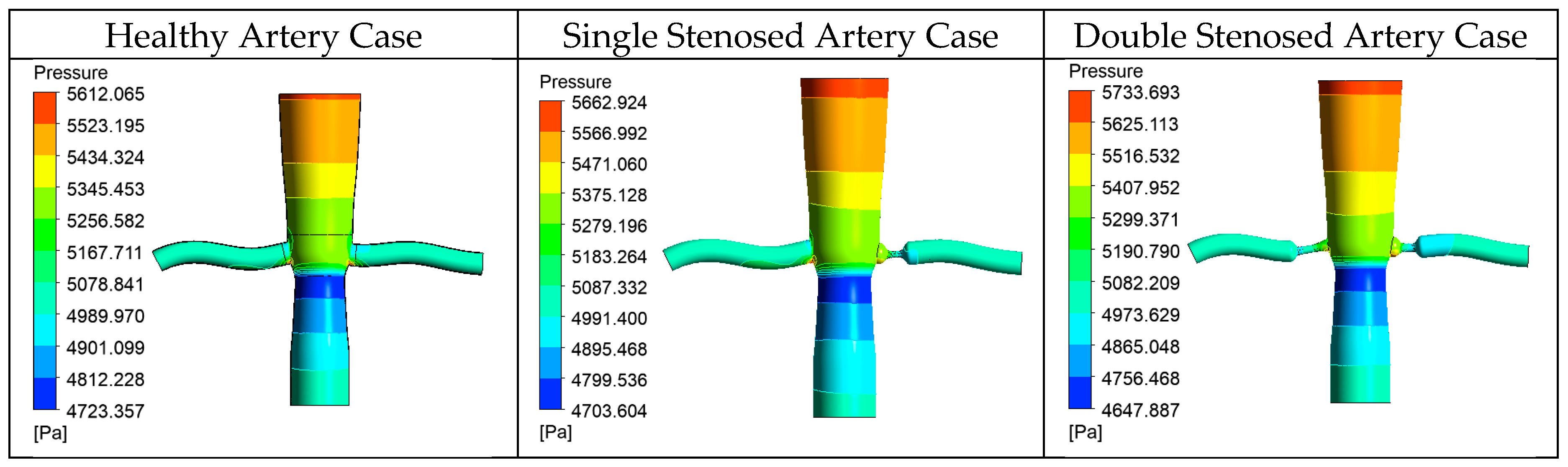
The pressure distribution along the abdominal aorta and renal arteries was analyzed to understand the hemodynamic impact of stenosis. Figure 7 presents the wall pressure distribution in the healthy, single stenosed, and double stenosed models during peak systole under normal blood pressure conditions. In all three models, the pressure gradually decreases along the length of the abdominal aorta. This trend is expected and reflects the normal resistance encountered by blood as it flows through the vessel. The boundary conditions applied in the simulations also contribute to this behavior. Again, the pressure distribution pattern closely aligns with the literature and validates the boundary conditions assigned [16,45].

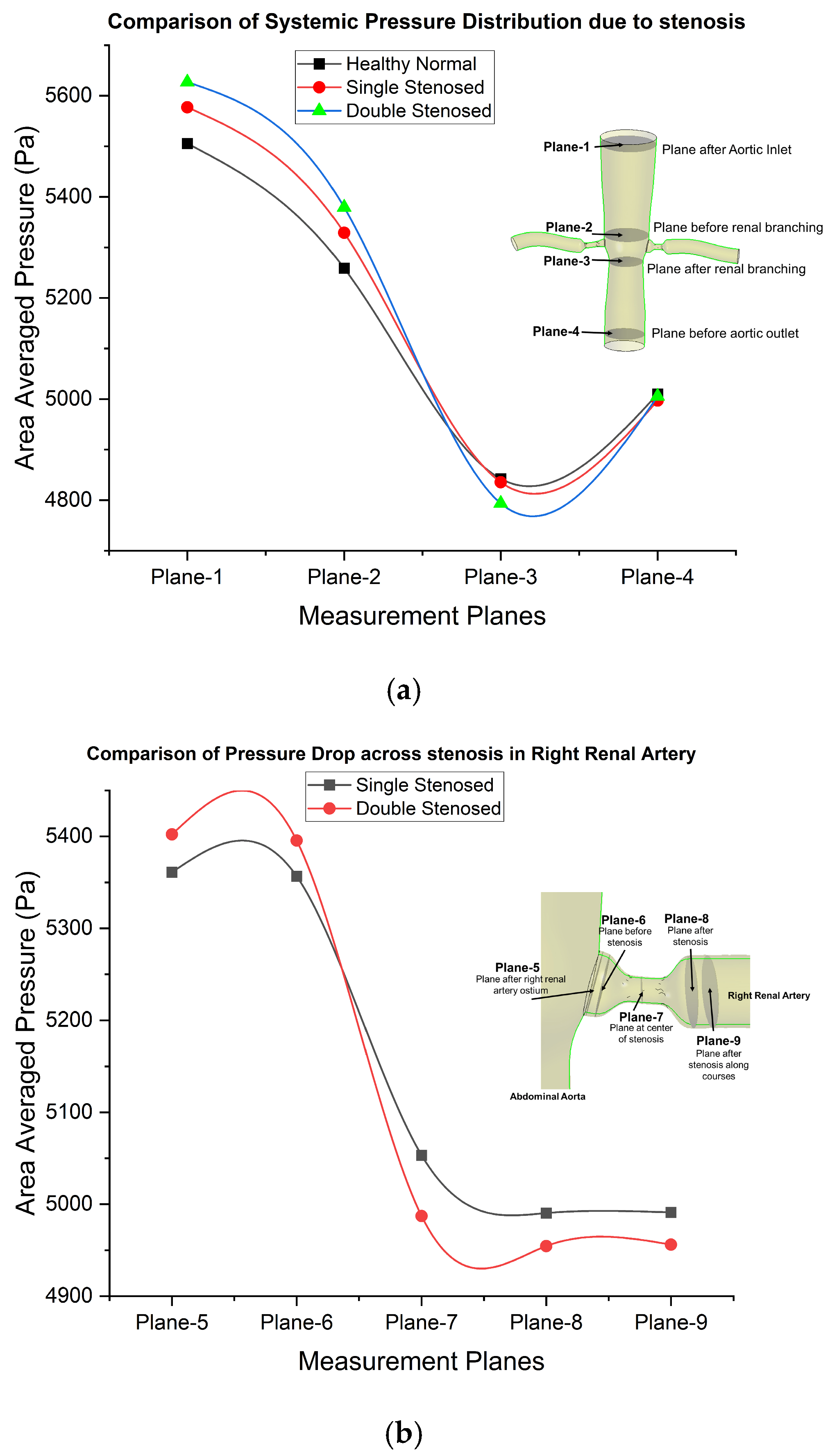
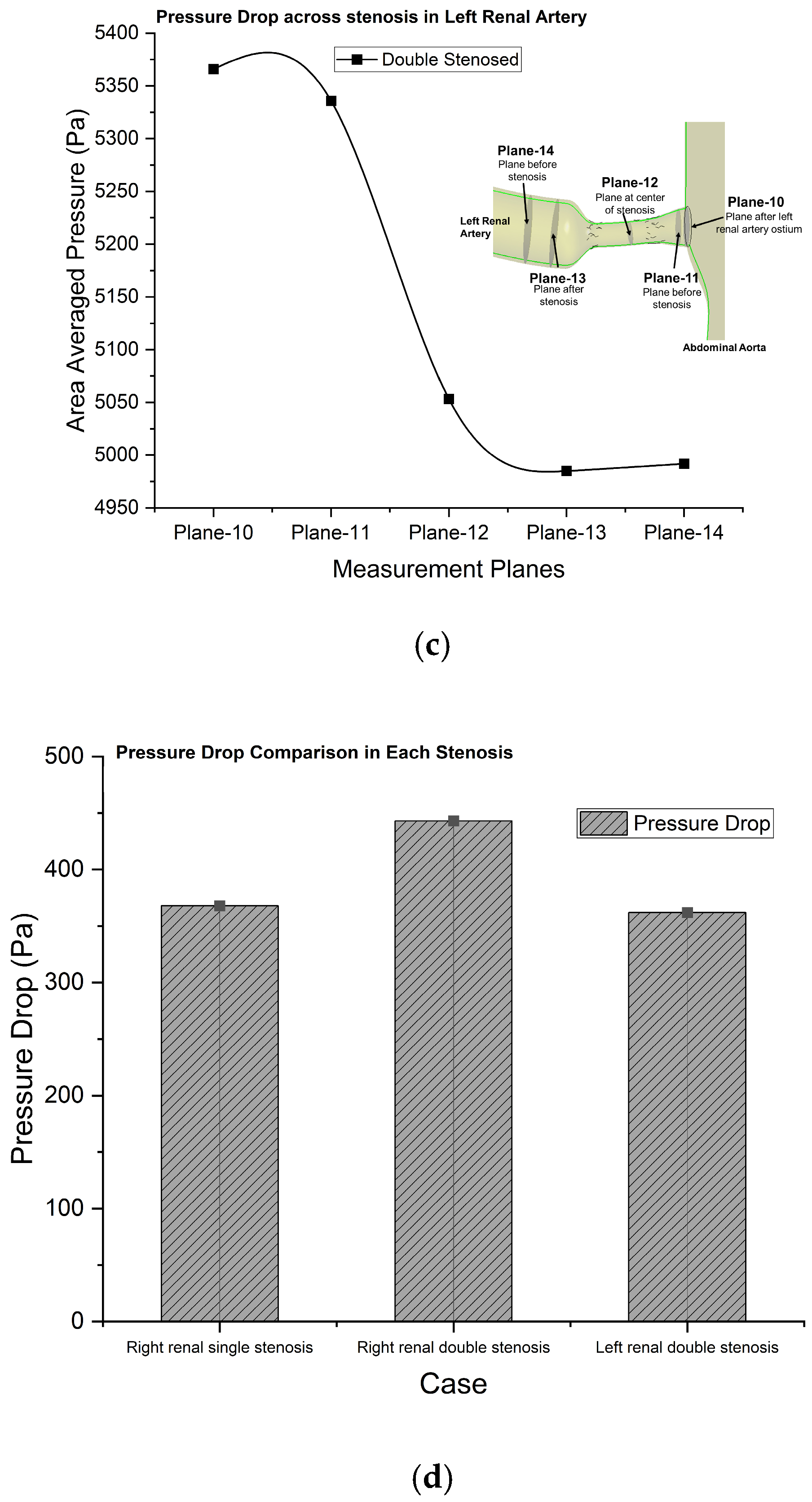
A different pattern is observed near the stenotic regions. A noticeable localized pressure drop appears at the stenotic neck of the right renal artery in the single stenosed model and at the necks of both renal arteries in the double stenosed model, as shown in Figure 7. This pressure reduction occurs as shown in Figure 8a,b, specifically in the narrowed section where the lumen is constricted. The drop is therefore spatially confined to the stenotic segment. Beyond this region, the pressure shows a partial recovery as the flow enters the wider portion of the artery.

The double stenosed model shows a larger pressure gradient across the stenotic necks compared with the healthy and single stenosed cases as shown in Figure 8b,c. This indicates a higher resistance to blood flow when both renal arteries are narrowed. Such behavior is consistent with basic fluid dynamic principles, where a reduction in vessel diameter accelerates the flow and increases energy losses [24,52]. The localized pressure reduction at the stenotic neck highlights its hemodynamic importance because pressure gradients directly influence renal perfusion. If the pressure drop persists across the stenosis, the downstream blood supply may decrease.

A comparison of the pressure drop values shown in Figure 8d further supports these observations. The pressure loss across the stenosis is greater in the double stenosed model than in the single stenosed case, indicating an increase in flow resistance within the renal branches. This behavior is again consistent with fluid dynamic theory, where narrowing of the vessel lumen produces stronger velocity gradients and higher energy dissipation. Overall, the results show that the presence of stenosis alters the pressure field in both the renal arteries and the abdominal aorta, with more pronounced effects in the double stenosed configuration.

3.3. Flow Redistribution

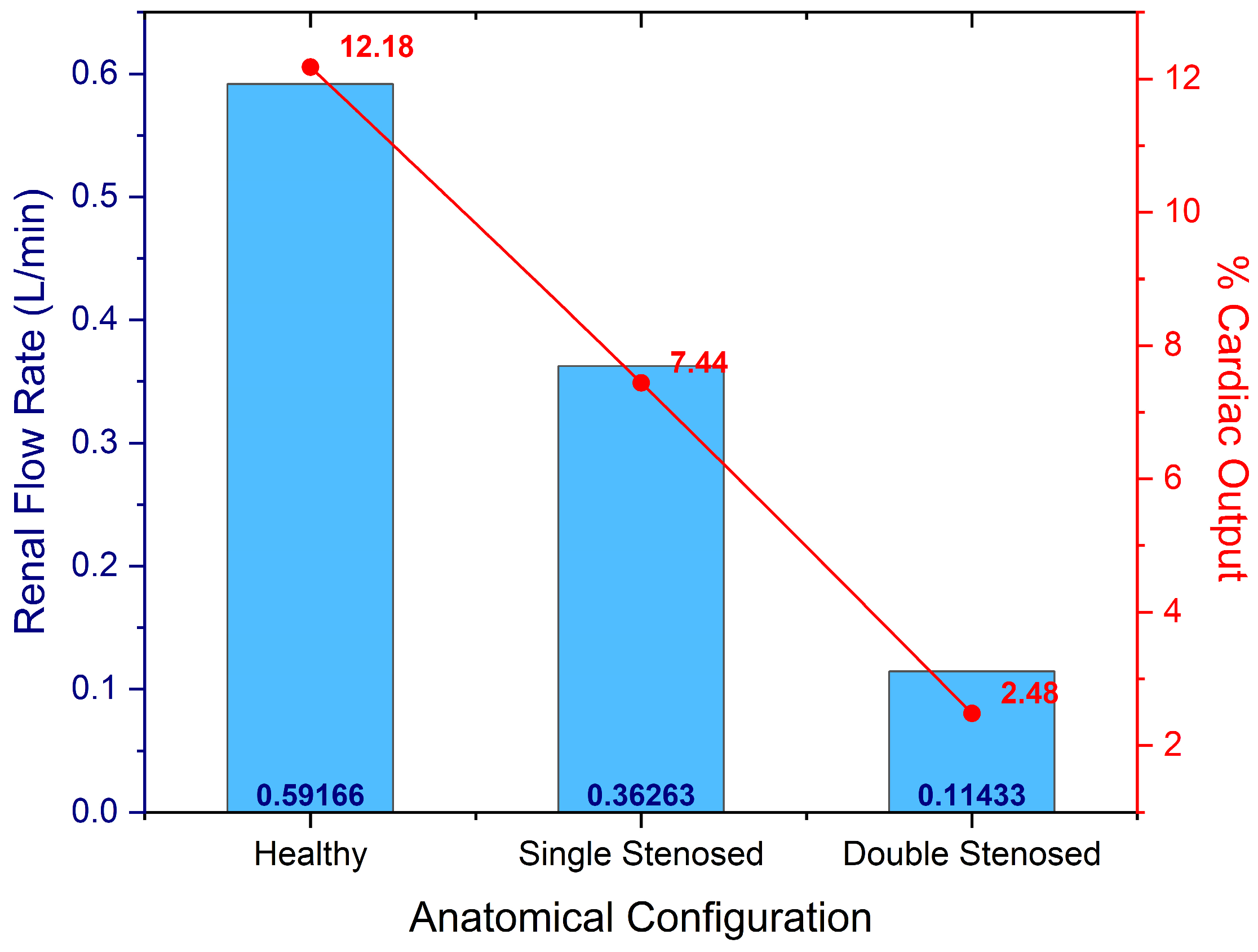
The computed flow distribution across the three cases demonstrates a physiologically consistent response to increased stenotic resistance. In the healthy case, the total renal fraction was 12.18% of the cardiac inflow, as shown in Figure 9, aligning with established resting state hemodynamic data. Under stenotic conditions, the model successfully captures the ‘flow-steal’ phenomenon, where the high-pressure gradient across the 72.5% (RRA) and 65% (LRA) diameter reductions forces a redistribution of the volume flux toward the distal aorta. Specifically, the renal flow fraction decreased to 7.44% in the single stenosed case and further to 2.47% in the double stenosed case. This significant reduction in perfusion is a characteristic clinical hallmark of high-grade renovascular hypertension, confirming that the rigid-wall CFD model accurately reflects the macro-scale hemodynamic impact of severe geometric narrowing [52,53].

3.4. Wall Shear Stress Distribution

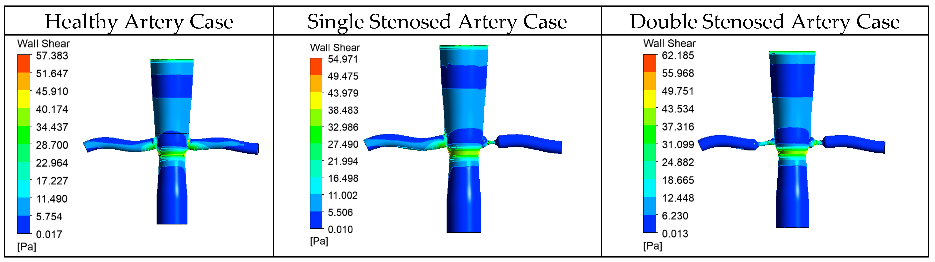
The instantaneous wall shear stress (WSS) distributions shown in Figure 10 provide direct insight into the localized mechanical loading imposed by stenosis. At peak systole under normal blood pressure conditions, the healthy configuration exhibits maximum WSS values of approximately 57 Pa at the renal ostial regions, corresponding to physiologic flow acceleration at the bifurcation. In contrast, the single stenosed model shows an elevated peak of nearly 54 Pa at the stenotic side, while the double stenosed case demonstrates further amplification, with bilateral peaks approaching 62 Pa at the pre-stenotic necks. These progressive increases reflect intensified velocity gradients and jet impingement caused by luminal narrowing. Notably, distal to the stenotic throat, WSS drops sharply to values below 2 Pa, indicating regions of flow deceleration and separation. Wall shear distribution trends have a close match with the literature [45,52].

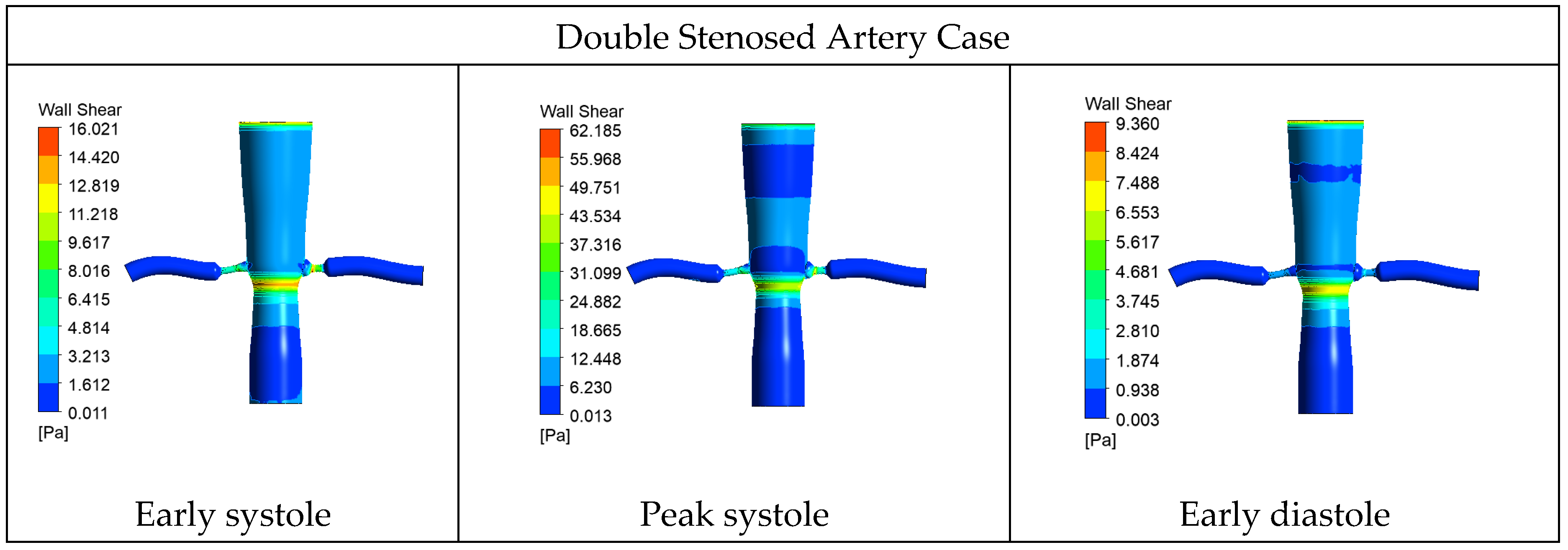
The temporal evolution observed in the double stenosed case in Figure 11 further emphasizes the pulsatile amplification of shear. During early systole, WSS begins to rise moderately at the stenotic neck, reaching its maximum during peak systole, and subsequently decreases in early diastole, although spatial heterogeneity persists. The concentration of elevated WSS at the stenotic throat is clinically significant, as sustained high shear (>15 Pa) has been associated with endothelial injury and plaque destabilization, whereas adjacent low-shear regions (<1–2 Pa) downstream promote atherogenic remodeling. Thus, the instantaneous WSS analysis highlights both the mechanical burden at the constriction site and the development of low-shear zones distal to the stenosis, providing a mechanistic context for the subsequent cycle-averaged TAWSS and OSI assessments used to evaluate long-term progression risk.

3.5. Time-Averaged Wall Shear Stress

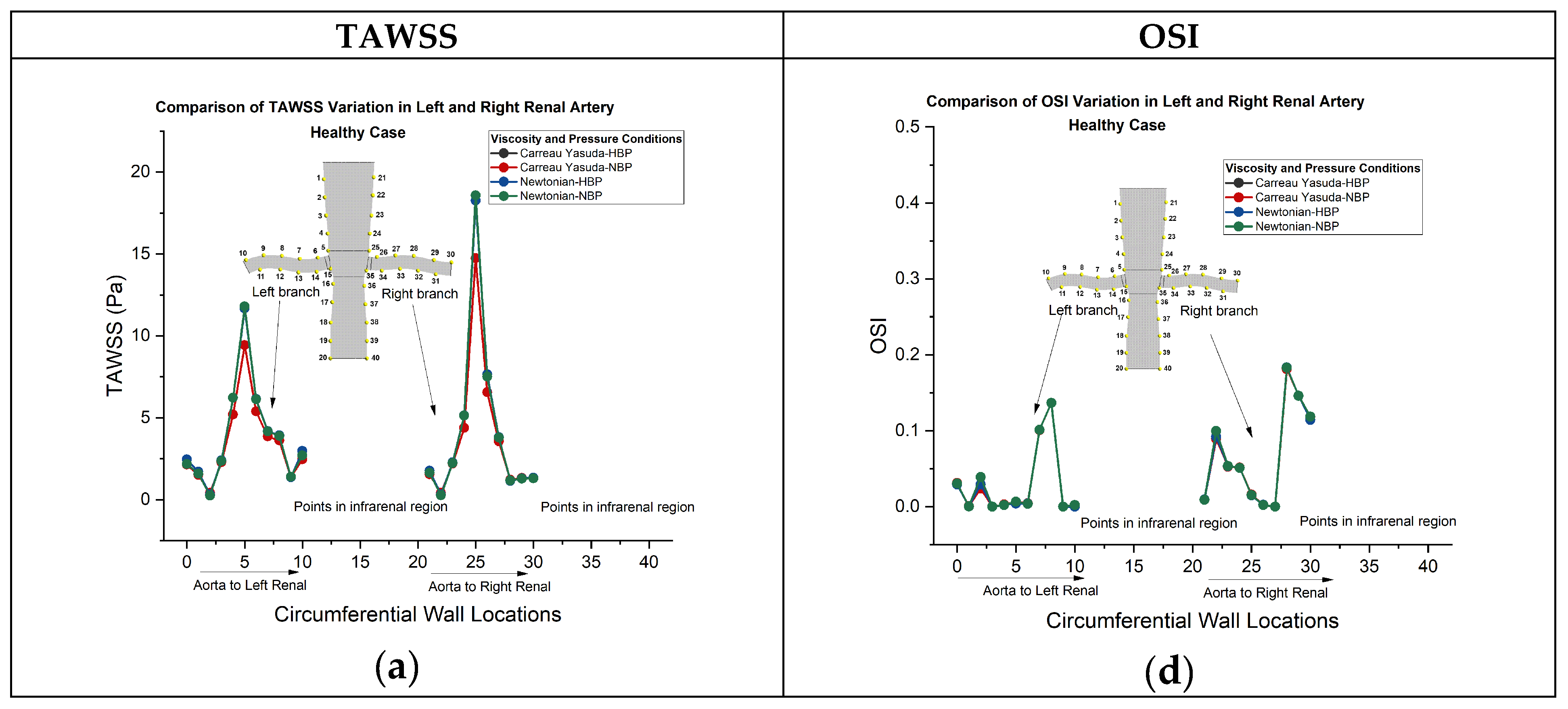
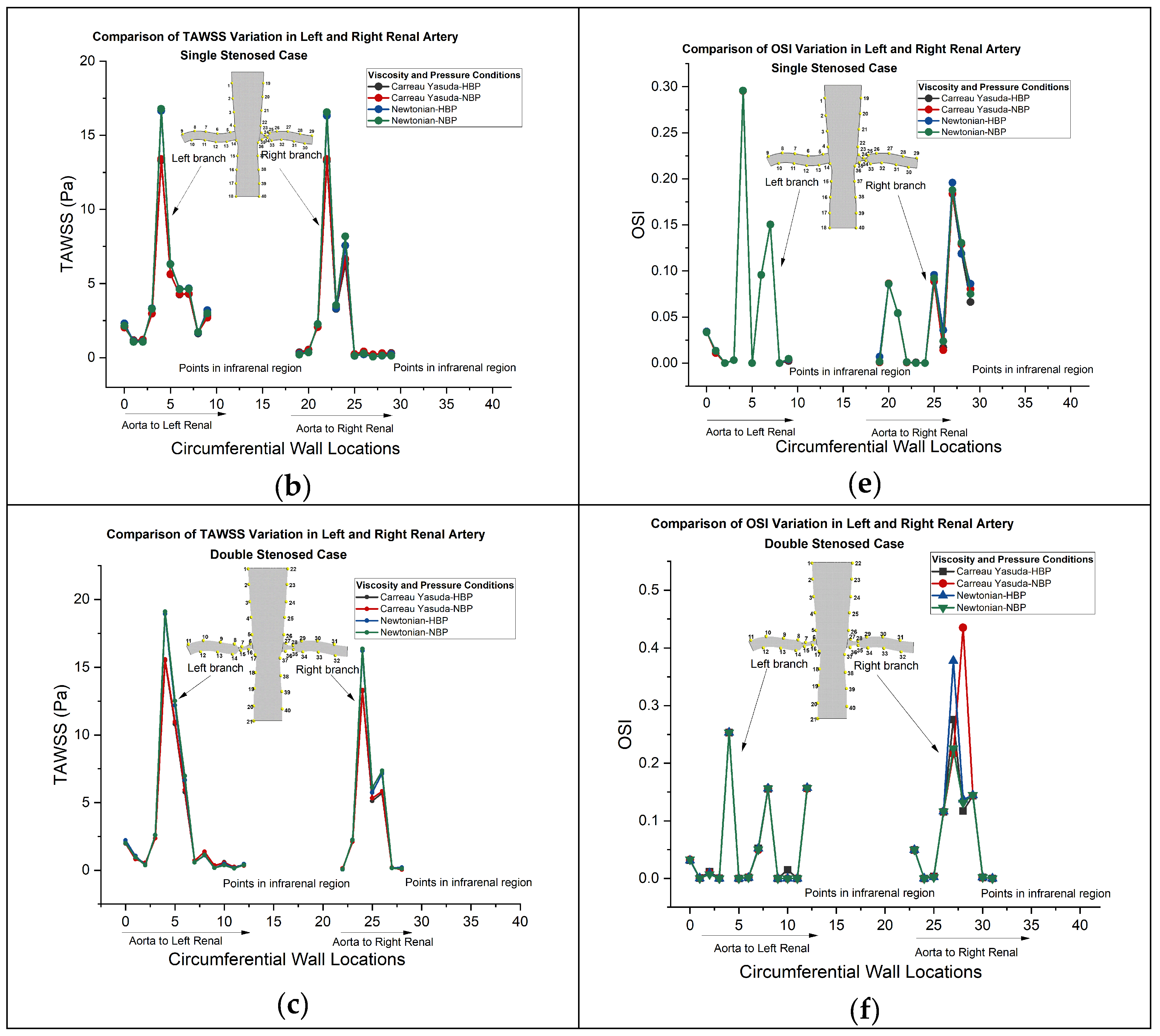
The axial variation in time-averaged wall shear stress (TAWSS) demonstrates a progressive amplification in peak shear magnitude with increasing stenosis severity, as shown in Figure 12a–c. In the healthy configuration, TAWSS peaks of approximately 14–15 Pa are observed immediately proximal to both renal artery bifurcations, corresponding to regions of localized flow acceleration. These values drop sharply to below 2 Pa within the infrarenal segments, indicating substantially reduced shear exposure downstream of the branching region [41,42,43]. In the single stenosed model, the peak TAWSS increases to approximately 16–17 Pa at the stenotic side, while the contralateral branch maintains values comparable to the healthy case, reflecting asymmetric flow redistribution. The double stenosed configuration exhibits the highest shear amplification, with bilateral peaks approaching 18–19 Pa at the pre-stenotic neck regions, indicating intensified velocity gradients and jet impingement effects on both renal ostia.

Despite this progressive increase in magnitude from healthy to double stenosis, the spatial footprint of TAWSS remains consistent, with maxima localized just upstream of the renal branches and markedly low values (≈0–2 Pa) in the distal infrarenal wall segments. Hypertensive conditions systematically elevate TAWSS across all cases, although the increase is moderate and does not alter the distribution pattern. Similarly, the Newtonian model predicts marginally higher peak TAWSS compared to the Carreau–Yasuda model, particularly in high-shear regions, reflecting the shear-thinning behavior of blood under non-Newtonian modeling. The observed escalation of peak TAWSS with stenosis severity highlights the increasing mechanical load imposed on the renal ostial regions, while the persistently low shear in infrarenal segments may predispose these areas to disturbed flow-related endothelial dysfunction.

3.6. Oscillatory Shear Index

The circumferential variation in oscillatory shear index (OSI) along the axial locations demonstrates a marked increase in flow oscillation with stenosis severity, as shown in Figure 12d–f. In the healthy configuration, OSI values remain predominantly low (<0.05) along most of the aortic and renal wall segments, with moderate elevations reaching approximately 0.15–0.18 near the distal renal regions, particularly under Newtonian–HBP conditions. This indicates relatively stable, unidirectional shear in the absence of geometric obstruction.

In the single stenosed model, localized amplification of OSI is observed near the stenotic side. Peak OSI values approach 0.28–0.30 in the left renal branch, while the contralateral branch exhibits moderate elevations (~0.15–0.20). These elevated values coincide spatially with regions downstream of the stenotic throat, where post-stenotic flow separation and recirculation are expected. The infrarenal segments largely maintain low OSI (<0.05), suggesting limited oscillatory behavior away from the disturbed zones.

The double stenosed configuration exhibits the most pronounced oscillatory behavior. Bilateral peaks are observed, with OSI values exceeding 0.40 and reaching approximately 0.43–0.45 under hypertensive conditions. These high OSI regions are localized distal to both stenotic necks, reflecting intensified bidirectional shear resulting from jet breakdown and recirculatory flow structures [43,52]. Compared to normotensive cases, hypertensive loading amplifies OSI magnitude without substantially shifting its spatial footprint. Differences between Newtonian and Carreau–Yasuda models are present but modest, with slightly elevated oscillation predicted under Newtonian assumptions in high-disturbance regions. Overall, the results indicate that increasing stenosis severity primarily magnifies oscillatory shear magnitude, particularly in post-stenotic zones, while preserving the general spatial pattern dictated by branching geometry.

The combined assessment of TAWSS and OSI provides a more comprehensive characterization of the local hemodynamic environment than either parameter alone. Regions exhibiting low TAWSS (<1–2 Pa) coupled with elevated OSI (>0.2) are widely recognized in the literature as atheroprone, as such conditions promote endothelial dysfunction, inflammatory signaling, and lipid accumulation [18,19,41,53]. In the present study, the infrarenal and post-stenotic regions in the stenosed models demonstrate precisely this hemodynamic signature—reduced cycle-averaged shear accompanied by increased oscillatory behavior—particularly in the double stenosed configuration under hypertensive loading.

Conversely, the stenotic neck regions exhibit very high TAWSS (up to ~18–19 Pa) with relatively low OSI, indicative of strong but predominantly unidirectional shear. While sustained high shear may contribute to endothelial injury or plaque destabilization, it is the coexistence of low TAWSS and elevated OSI distal to the stenosis that represents a more critical environment for plaque initiation and progression. The progressive amplification of OSI alongside increasing stenosis severity therefore suggests an expanding region of disturbed hemodynamics, potentially accelerating atherosclerotic remodeling and adverse vascular adaptation. These findings reinforce the mechanobiological link between geometric obstruction, altered pulsatile flow, and spatially heterogeneous vascular risk.

4. Limitations of the Study and Future Work

The present study has some limitations that should be acknowledged. First, the current simulations employ a rigid wall assumption for the arterial walls. While this simplification is commonly adopted in vascular CFD studies to isolate flow-related effects, arterial wall compliance may influence local hemodynamic parameters. Future work will incorporate the patient-specific fluid–structure interaction (FSI) framework discussed in the introduction to further examine the effect of wall deformation on the TAWSS and OSI patterns. Although the idealized computational geometry enables systematic evaluation of flow behavior under controlled geometric conditions, future investigations will consider patient-specific models derived from clinical imaging. This will also account for inter-individual anatomical variability in addition to physiological variations. The stenosis was modeled as an axisymmetric concentric narrowing to provide a controlled representation of lumen reduction. Arterial stenoses may exhibit irregular or eccentric morphologies. However, the simplified representation used here allows clearer interpretation of the hemodynamic influence of stenosis severity without introducing additional geometric complexities. Finally, the outlet boundary conditions were prescribed using representative pulsatile pressure profiles from the literature sources rather than patient-specific measurements. While this approach reproduces physiologically realistic pulsatile flow conditions, future studies incorporating subject-specific pressure or flow waveforms may provide further insight into individual hemodynamic responses.

5. Conclusions

In conclusion, increasing stenosis severity gradually altered the hemodynamic environment within the abdominal–renal arterial system. Velocity contours showed increased jet formation and enlarged post-stenotic recirculation zones, accompanied by pronounced localized pressure drops across the stenotic necks. These flow changes resulted in elevated peak WSS and TAWSS at the pre-stenotic regions, most prominently in the double stenosed case, while distal segments showed reduced shear experience and increased oscillatory behavior, as reflected by elevated OSI. Importantly, the study provides a comparative assessment of left and right renal branch hemodynamics under healthy, single, and double stenosis, further evaluated across normal blood pressure and high blood pressure conditions and under both Newtonian and Carreau–Yasuda rheological assumptions. While the spatial distribution patterns remained majorly same, stenosis severity, pressure, and viscosity have collectively changed the magnitude of shear and oscillatory indices. Altogether, these findings highlight the compounded influence of geometric obstruction, systemic pressure, and blood rheology on renal arterial hemodynamics and their potential role in vascular dysfunction.