SOH- and Temperature-Aware Adaptive SOC Boundaries for Second-Life Li-Ion Batteries in Off-Grid PV–BESSs

Abstract

In this study, an adaptive state-of-charge (SOC) boundary strategy (ASBS) is proposed that dynamically adjusts the admissible upper and lower SOC limits of second-life lithium-ion batteries in off-grid photovoltaic battery energy storage systems (PV-BESSs) based on real-time state of health (SOH) and temperature feedback. The strategy is formulated using a unified electrical–thermal–aging model with an online state estimator and ensures both electrical safety and power feasibility while remaining fully compatible with standard energy management functions. Two representative simulations—a single-day operating profile and a continuous thirty-day sequence—demonstrate the effectiveness of the ASBS. In the twenty-four-hour case, the duration spent in high state-of-charge conditions is reduced by approximately 0.30–0.50 h, the abrupt end-of-charging transition is eliminated, and the temperature rise is slightly moderated, all without any loss of energy supply. Over thirty days, the difference between the ASBS and a fixed state-of-charge window remains effectively zero for almost all hours, with only a brief midday deviation of −4 to −5 percentage points and no cumulative drift. Indicators of electrical and thermal stress improve substantially, including an approximate 70% reduction in the root mean square charging current. These results confirm that the ASBS provides a practical and non-intrusive means of mitigating stress on second-life lithium-ion batteries while preserving full energy autonomy in off-grid photovoltaic systems.

1. Introduction

With the rapid growth of electric vehicles (EVs) and distributed energy storage, an increasing number of lithium-ion batteries are reaching their end of life (EoL). Compared with direct scrapping or pyrometallurgical recycling, a closed-loop pathway based on cascade reuse and regeneration offers broader advantages for resource efficiency, environmental impact, and economic viability [1]. Lifecycle and scenario analyses further show that standardized second-life utilization can reduce carbon emissions and deliver system-level gains [2]. In practice, retired traction batteries are graded and repurposed for household or small-scale stationary applications, creating cost-effective options for off-grid photovoltaic battery energy storage systems (PV–BESSs) [3].

Recent advances in online state-of-charge (SOC) and state-of-health (SOH) estimation, equivalent-circuit modeling, and electrical–thermal–aging coupling have provided a solid foundation for battery diagnosis and lifetime assessment [4,5,6]. In off-grid or weak-grid residential settings, charging strategies substantially affect capacity fade and usable energy [7]. System-level studies have examined configuration choices and lifetime trade-offs for second-life batteries [8], while investigations of repurposed EV packs in grid services have highlighted operational constraints relevant to residential applications [9].

Despite these developments, many operational studies continue to employ fixed mid-range SOC windows for lifetime extension. Wang et al. [10] conducted partial-cycle aging tests within a 20–80% SOC range and demonstrated that mid-range cycling significantly slows SOH degradation compared with deeper cycling. Chen, Z et al. [11] introduced a holistic sustainability metric and, using recent aging data, identified the 20–80% range as a conservative operating threshold under unknown chemical conditions. Sowe, J et al. [12] reviewed lifetime-extension techniques involving SOC, current, voltage, and temperature derating, while Collath et al. [13] surveyed aging-aware operation strategies for battery energy storage systems and emphasized SOC window selection and power derating as key levers for longevity-oriented control. Rajah et al. [14] proposed degradation-aware derating schemes that adjust charge/discharge power based on aging indicators; however, these schemes still rely on pre-defined static SOC limits and do not explicitly adapt the SOC window to temperature and SOH evolution in second-life off-grid residential applications.

However, there is no unified framework capable of dynamically adjusting the SOC window of second-life batteries to both temperature conditions and SOH progression while simultaneously ensuring voltage feasibility, power-derating compliance, and energy autonomy requirements. Existing approaches remain largely static, do not accommodate parameter drift, and lack the engineered smoothness required for seamless deployment in legacy battery management system (BMS) and energy management system (EMS) architectures.

This limitation is particularly critical in residential off-grid PV systems, where second-life batteries experience coupled thermal, aging, and load uncertainties. A practical, adaptive SOC boundary strategy is, therefore, needed to extend usable life while maintaining system autonomy.

We target lifetime-aware control by reshaping the admissible SOC window using only temperature and SOH feedback while remaining compatible with EMS constraints. SOH and temperature are selected as adaptive inputs because they directly reflect long-term degradation severity and short-term thermal safety margin, respectively, which constitute the most critical constraints for second-life batteries. Other operational disturbances (e.g., PV/load fluctuations) are primarily addressed by the EMS power-balancing loop, whereas incorporating additional stress history indicators would increase sensing and modeling complexity. Therefore, this work focuses on a lightweight two-factor adaptation, while multi-factor extensions are deferred to future work. Built on a unified framework—including a second-order equivalent circuit model, a dual-node thermal network, semi-empirical aging models, and an extended Kalman filter—in this study, the following are achieved:

• An SOH- and temperature-aware adaptive SOC boundary strategy (ASBS-ST) is proposed—implemented via an adaptive SOC window manager within the hierarchical EMS—that is interpretable, lightweight, and directly applicable to existing BMS/EMS platforms without requiring intrusive sensing.
• Feasibility and derating are explicitly integrated using voltage-feasible boundary intersection, energy autonomy constraints, and engineered smoothness (hysteresis and ramp limits), enabling stable online boundary adjustment.
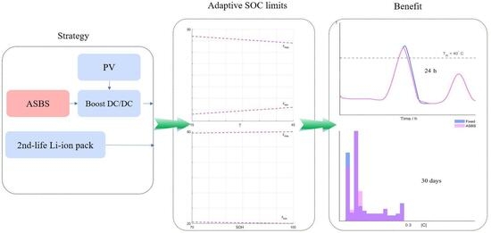
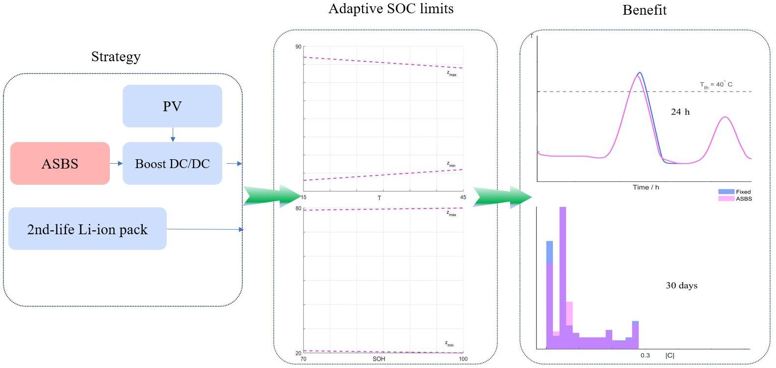
• The strategy is verified under realistic off-grid PV–BESS conditions, including 24 h (24 h) and 30-day scenarios, leading to reduced high SOC exposure, smoother current profiles, and mitigated electro-thermal aging without compromising energy autonomy.

Finally, the proposed controller requires only SOH and temperature feedback—without rate prediction or PV/load forecasting—and relies on simple look-up operations with slope limiting, ensuring real-time feasibility for embedded BMS/EMS platforms. In this paper, the “unified framework” refers to a closed-loop integration of electro-thermal–aging state estimation, adaptive SOC boundary scheduling that accounts for both SOH and temperature, and EMS execution for second-life PV–BESS operation.

Section 2 introduces the system architecture and unified electrical–thermal–aging models, including electrical–thermal–aging coupling and measurement equations and operational constraints. Section 3 presents the SOH- and temperature-aware adaptive SOC boundary control strategy together with the associated voltage–power feasibility formulations. Section 4 describes the Simulink implementation, solver configurations, and the simulation setup for both the 24 h and 30-day scenarios. In Section 5, the simulation results are reported and discussed, their implications for lifetime-aware operation are interpreted, and the main conclusions and limitations of the study are summarized.

2. System Architecture and Modeling

2.1. System Architecture

The studied system is a residential off-grid PV–battery energy storage system (PV–BESS) consisting of a photovoltaic (PV) array, an MPPT-based boost DC/DC converter, a 650 V DC bus, a second-life lithium-ion battery pack equipped with a BMS, a DC/AC inverter, and typical household loads. The EMS coordinates power flows among the PV array, battery, and loads to maintain the stability of the DC bus voltage.

The BMS monitors cell voltages, temperatures, and current and provides SOC, SOH, and temperature to the EMS. The key symbols and parameters used in the equations throughout the manuscript are summarized in Appendix A (

Table A1. Key symbols used in Equations (1)–(19).

Symbol	Meaning (Unit)
$z$	State of charge (SOC) (–)
$\left[z_{min},z_{max}\right]$	SOC operation window (fixed or adaptive) (–)
$U$	Terminal voltage (V)
$U_{OC}$	Open-circuit voltage (V)
$U_1,U_2$	Polarization voltages of RC branches (V)
$R_0$	Ohmic resistance (Ω)
$R_1,R_2$	Polarization resistances (Ω)
$C_1,C_2$	Polarization capacitances (F)
$i$	Battery current (discharge > 0) (A)
$Q_n$	Nominal capacity (Ah)
$R_{12},R_{1a}$	Core–shell and shell–ambient thermal resistances (K/W)
$C_{core},C_{shell}$	Core and shell heat capacities (J/K)
$T_1,T_2,T_a$	Core, case, and ambient temperatures (°C or K)
$Q_{gen}$	Total heat generation rate (W)
${SOH}_Q,{SOH}_R$	State of health: capacity/resistance (–)
$P_b^{*}$	Battery power command (saturated) (kW)
$P_{max}$	Maximum allowable power (derated) (kW)
$k_T,k_R$	Temperature and health derating slopes (1/°C, –)
$z_{\mathrm{v}\mathrm{o}\mathrm{l}\mathrm{t}}^{\mathrm{m}\mathrm{i}\mathrm{n}},z_{\mathrm{v}\mathrm{o}\mathrm{l}\mathrm{t}}^{\mathrm{m}\mathrm{a}\mathrm{x}}$	Voltage-feasible SOC range (–)
$z_{\mathrm{p}\mathrm{o}\mathrm{w}}^{\mathrm{m}\mathrm{i}\mathrm{n}},z_{\mathrm{p}\mathrm{o}\mathrm{w}}^{\mathrm{m}\mathrm{a}\mathrm{x}}$	Power-feasible SOC range (–)
ΔU	Cell voltage margin (V)

). The EMS applies temperature- and SOH-dependent SOC boundaries as follows:

$$\left[z_{min}, z_{max}\right]=f\left(T,SOH\right),$$

(1)

where the mapping may be implemented through affine or lookup table rules [15,16,17].

These candidate SOC limits must satisfy voltage–temperature safety constraints [7,18,19]

$$V_{min}\le V_{\mathrm{cell}}\le V_{max},T_{min}\le T\le T_{max}, \left|I\right|\le I_{max}$$

(2)

and must remain feasible with respect to energy availability

$$Feasible⟺E_{req}\left(t\right) \le { E}_{avail}\left(t\right),$$

(3)

ensuring compatibility with practical PV–BESS operation.

In the remainder of this section, the electrical, thermal, and aging models required to compute SOC, temperature, and SOH in real time are established.

2.2. Electrical Model: Second-Order Equivalent Circuit (2-RC ECM)

The two-RC equivalent circuit model (ECM) is adopted due to its balance between computational efficiency and fidelity in representing lithium-ion cell behavior [20,21,22]. The model provides the state–space foundation for SOC estimation and voltage prediction in Section 3.

With cell current $i$ ($i>0$ discharge, $i<0$ charge) and SOC $z \in [0, 1]$ taken as state variables, the dynamics of the polarization voltages are given by (4) [20,21,22,23] as follows:

$${\dot{U}}_1=-{\displaystyle \frac{1}{R_1{C}_1}}{U}_1 + {\displaystyle \frac{1}{C_1}}i,{\dot{U}}_2= -{\displaystyle \frac{1}{R_2{C}_2}}{U}_2+ {\displaystyle \frac{1}{C_2}}i.$$

(4)

The SOC dynamics are given by (5) [10,11,12,13]

$$\dot{z}=\left\{\begin{array}{c}-{\displaystyle \frac{i}{Q_n {SOH}_Q}},i\ge 0,\\ -{\displaystyle \frac{{\eta }_{chg} i}{Q_n {SOH}_Q}},i<0.\end{array}\right.$$

(5)

and the terminal voltage equation is expressed in (6) [10,11,12,13] as follows:

$$U = { U}_{OC}\left(z,T\right) - i R_0\left(z,T,{SOH}_R\right) - U_1 - U_2,$$

(6)

where $U_1$ and $U_2$ denote the polarization voltages of the two RC branches in the equivalent-circuit model.

Applying zero-order-hold (ZOH) discretization with sampling period $\Delta t$ yields (7) [20,23,24] as follows:

$$x_{k+1}=A_k{x}_k+B_k{i}_k,U_k=U_{OC}\left(z_k,T_k\right)+C_k{x}_k+D_k{i}_k,$$

(7)

where $x_k= [U_{1,k},U_{2,k},z_k{]}^T$ and $u_k=i_k$ and $y_k=U_k$. Matrices $(A_k,B_k,C_k,D_k)$ are the ZOH discretization of the continuous-time 2-RC model; the dimensions are consistent with a single-output voltage measurement. Although the present parameterization is based on second-life NMC cells, the proposed ASBS is chemistry-agnostic at the control level because it adapts SOC boundaries using estimated $\left\{SOC,SOH,T\right\}$ feedback. For other chemistries (e.g., LFP or NCA), chemistry-dependent components—such as the OCV–SOC curve, impedance/parameter maps (e.g., $R_0$), and thermal/aging coefficients—should be re-identified or re-tuned, while the boundary scheduling and closed-loop execution logic remain unchanged.

2.3. Thermal Model: Dual-Node (2R/2C)

To capture the temperature rise of retired cells caused by increased ohmic losses and weakened heat dissipation, a core–shell dual-node thermal network (2R/2C) is adopted. This model provides an efficient compromise between accuracy and complexity and is coupled with the 2-RC electrical model [25,26,27].

This model includes two thermal nodes, $T_1$ (core) and $T_2$ (shell), with ambient temperature $T_a$. The thermal resistances and heat capacities are $R_{12},R_{1a}$ and $C_{core},C_{shell},$ respectively. The heat transfer and dissipation dynamics are expressed by (8) [25,26,27,28] as follows:

$$\left\{\begin{array}{c}{\dot{T}}_1= -{\displaystyle \frac{T_1-T_2}{R_{12} C_{core}}}+{\displaystyle \frac{Q_{gen}}{C_{core}}} \\ {\dot{T}}_2= {\displaystyle \frac{T_1-T_2}{R_{12} C_{shell}}}-{\displaystyle \frac{T_2-T_a}{R_{1a}{C}_{shell}}}\end{array}\right..$$

(8)

Although the dual-node (2R/2C) thermal network contains two thermal time constants, $R_{12}{C}_{core}$ and $R_{1a}{C}_{shell}$, the former is usually much larger [25,26,27,28]. Consequently, the temperature dynamics are dominated by the slow mode, leading to an effective first-order lag behavior.

The total heat generation consists of Joule and reversible components (with current convention from Section 2.2: $i>0$ discharge, $i<0$ charge) (9) [25,27] as follows:

$$Q_{gen}=i^2{R}_0+ i T {\displaystyle \frac{\partial U_{OC}}{\partial T}}.$$

(9)

The first term represents irreversible ohmic loss, while the second accounts for reversible entropic heat, whose sign depends on the entropy coefficient $\partial U_{OC}/\partial T$.

2.4. Aging Model: Cycle + Calendar (Semi-Empirical) and Online Update

In this section, mechanistic, data-driven, and semi-empirical aging approaches are compared, and then a cycle–calendar semi-empirical framework coupled with the 2-RC electrical and 2R–2C thermal models is developed. Mechanistic P2D/multiphysics models are interpretable but parameter-intensive and computationally expensive [29], while data-driven models require large training datasets and have limited transferability across temperature and C-rate domains [30]. Semi-empirical models offer a practical compromise: they couple naturally with ECM–thermal structures, support stable rolling updates, and require modest calibration data [13,29,30]. Accordingly, aging is decomposed into cycle and calendar components, and capacity SOH and resistance SOH are jointly updated using the expressions in Equations (10)–(13). Temperature dependence is introduced into the semi-empirical model through the thermal stress variable $\theta$.

$$\Delta SO{H}_{\mathit{cyc}}=k_c {\theta }^{m_R}exp(-{\displaystyle \frac{E_a}{R_{g}T}})w(\mathit{DoD},C,T),$$

(10)

where $w(\mathit{DoD},C,T)$ is the weighting function calibrated by the DoD–C-rate coupling law and $k_c,m_R,E_a,{and R}_g$ are fitted constants.

The capacity and resistance are updated online via (11) [28,29,30,31,32,33,34,35] as follows:

$$\left\{\begin{array}{c}SO{H}_{Q,k+1}=SO{H}_{Q,k}-\Delta SO{H}_{\mathit{cyc},k}, \\ R_{0,k+1}=R_{0,k}[1+k_{R,\mathit{cyc}} {\theta }^{m_R}exp(-{\displaystyle \frac{E_R}{R_g{T}_k}}\left)\right],\end{array}\right.$$

(11)

where the thermal stress variable $\theta$ is obtained from the temperature field in Section 2.3.

The calendar-aging process, occurring under static or low-load conditions, arises from SEI thickening and electrolyte decomposition. This process is jointly affected by temperature and SOC. To preserve interpretability and computational efficiency, a “stress-integral + square-root-time” representation is employed (12) [28,29,30,31,32,33,34,35] as follows:

$$\Delta SO{H}_{\mathit{cal}}=k_{\mathit{cal}}exp(-{\displaystyle \frac{E_{\mathit{cal}}}{R_{g}T}}){\int }_0^{t}f(z,T) dt,$$

(12)

where $k_{\mathit{cal}}$ and $E_{\mathit{cal}}$ are constants and $f(z,T)$ is the coupled SOC temperature stress function.

Cycle- and calendar-aging contributions are combined to jointly update $SO{H}_Q$ and $R_0$ according to Equations (11)–(13), ensuring consistency between SOC estimation and health evolution. The thermal stress variable $\theta$ is supplied by the thermal field in Section 2.3.

The update equations are expressed by (13) [28,29,30,31,32,33,34,35] as follows:

$$\left\{\begin{array}{c}SO{H}_{Q,k+1}=SO{H}_{Q,k}-(\Delta SO{H}_{\mathit{cyc},k}+\Delta SO{H}_{\mathit{cal},k}),\\ R_{0,k+1}=R_{0,k}\left[1+k_R^{tot}\left({\theta }_k,T_k\right)\right], \end{array}\right.$$

(13)

where $k_R^{tot}({\theta }_k,T_k)$ represents the composite growth coefficient driven by both cycle and calendar stresses.

2.5. Parameter Identification, Temperature Mapping, and Online Coupling

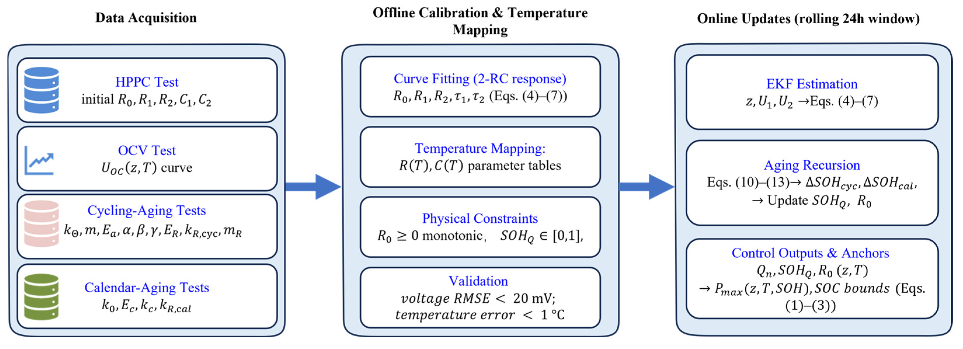
To ensure consistency among the electrical, thermal, and aging subsystems, all parameters are identified, temperature-mapped, and recursively updated following the workflow in Figure 1. The HPPC test provides the initial electrical parameters $(R_0,{ R}_1,R_2,{ C}_1,{ C}_2)$ for the 2-RC ECM used in Equations (4)–(7). The OCV test determines the de-hysterized $U_{OC}(z,T)$ curve used in the voltage Equation (6) and for the inverse lookup $z=U_{OC}^{-1}(U,T)$. Cycle- and calendar-aging experiments yield the empirical coefficients $(k_{\theta },m,{ E}_a,\alpha ,\beta ,\gamma ,{ m}_R,{ E}_R,{ k}_{R,cyc})$ and $(k_0,{ E}_c,{ k}_c,k_{R,cal})$ that drive the degradation recursions in Equations (10)–(13).

Offline, the identified parameters are mapped to temperature tables $R\left(T\right)$ and $C\left(T\right)$ under the constraints $R_0 \ge 0$ and $SO{H}_Q\in [0, 1]$; acceptance requires a terminal voltage RMSE $< 20$ mV and a temperature error $< 1 °C$. This guarantees consistency between offline calibration and online estimation, preventing parameter drift over long-term cycling. During operation, the EKF updates $(z,{ U}_1,{ U}_2)$ via Equations (4)–(7), and the aging recursions (10)–(13) update $SO{H}_Q$ and $R_0$. The updated anchors $\{Q_n,SO{H}_Q,{ R}_0(z,T\left)\right\}$ then determine $P_{max}(z,T,SOH)$ and the admissible SOC bounds used in Equations (1)–(3).

Table 1. Symbols, initialization sources, online update, and usage.

Parameter Category	Symbol	Initialization Source	Online Update	Usage/Relevance
Ohmic/Polarization Resistance and Capacitance	$R_0,{ R}_1,{ R}_2,$ $C_1, { C}_2$	From the HPPC exponential fit	$R\left(T\right), C\left(T\right)$ mapping via temperature interpolation	Used in ECM Equations (4)–(7) for SOC and voltage estimation; supports $P_{max}(z,T,SOH)$ in Equations (1)–(3).
OCV Curve	$U_{OC}\left(z,T\right)$	OCV test (fitted and de-hysterized curve)	Temperature-corrected lookup table	Provides terminal voltage link in Equation (6); input for EKF estimation (4)–(7).
Thermal Model	$R_{12}{, R}_{1a}$ $C_{core}, C_{shell}$ $T_1,{ T}_2,{ T}_a$	The literature/datasheet	No online update	Thermal dynamics (Equations (8) and (9)); temperature input for ASBS trigger.
Cycle-Aging Coefficients	$k_{\Theta }, m,{ E}_a,$ $\alpha , \beta , \gamma ,{ E}_R,$ $k_{R,cyc},{ m}_R$	The literature/ experiment	Recursive update via Equations (10) and (11) $\Delta {SOH}_{cyc}$	Updates $SO{H}_Q$ and $R_0$ according to cycling stress in Equation (11); coupled with the thermal field from Equation (8).
Calendar-Aging Coefficients	$k_0,{ E}_c,$ $k_c,{ k}_{R,cal}$	The literature/ experiment	Online update via Equations (12) and (13) $\Delta {SOH}_{cal}$	Updates $SO{H}_Q$ and $R_0$ under static conditions using the SOC–T stress integral Equation (12); ensures continuity in Equation (13).

summarizes all symbols, parameter initialization sources, online update rules, and usage across the ECM, thermal, and aging models, providing a complete overview of the parameter flows used throughout the proposed modeling and control framework, ensuring clarity and reproducibility.

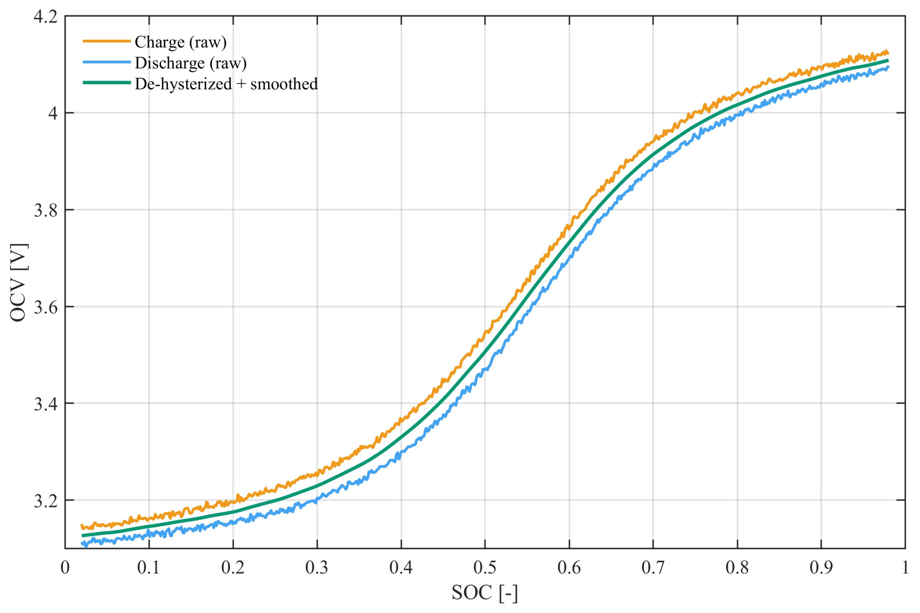
To support the voltage Equation (6) and the inverse lookup $z=U_{OC}^{-1}(U,T)$, Figure 2 shows the OCV–SOC characteristics: the raw charge/discharge curves and the processed curve after hysteresis removal and smoothing. The resulting monotonic curve forms the $U_{OC}(z,T)$ table used for the EKF in Equations (4)–(7) and for the feasibility checks in Equations (1)–(3). The acceptance criteria are satisfied (terminal voltage RMSE < 20 mV; temperature correction error < 1 °C).

The OCV–SOC characteristics of the second-life NMC cell indicate that both the raw charge and discharge branches and the processed (de-hysterized and smoothed) curve were obtained. The OCV data were measured through low-rate characterization tests at 25 °C, covering the voltage range of 3.1–4.2 V over the SOC interval of 0–1. For consistency, SOC is represented in normalized form (0–1) in all model equations, while percentage notation (0–100%) is only used when discussing practical operational limits (e.g., 20–80%), with both forms being equivalent. The OCV data were obtained from low-rate characterization tests at 25 °C, covering the voltage range of 3.1–4.2 V over SOC ∈ [0, 1]. For clarity, SOC is expressed in normalized form (0–1) within the model and in percentage form (0–100%) when referring to operational limits (e.g., 20–80%). Both notations are equivalent and follow standard practice.

3. Control Strategy and Implementation

Building upon the unified electro-thermal–aging framework established in Section 2, in this section, a control strategy that integrates aging-aware SOC boundary adaptation and hierarchical EMS implementation is developed.

Recent reviews emphasize that aging-aware operation of battery energy storage systems (BESSs), i.e., adjusting power limits and admissible SOC ranges according to degradation risk, can effectively balance lifetime and service performance [15]. To ensure the safe and efficient operation of second-life lithium-ion batteries in off-grid photovoltaic energy storage systems, a hierarchical control strategy is proposed that balances longevity extension and supply–demand stability. A standard hierarchical EMS architecture (primary/secondary/tertiary layers) is adopted for PV–BESS power balancing and converter coordination. The core novelty lies in the proposed adaptive SOC window manager, which enables aging- and temperature-aware SOC boundary scheduling within the EMS loop. The main objective is to guarantee continuous power delivery (ENS ≈ 0) while minimizing thermal and aging stresses and maintaining DC bus voltage stability.

As illustrated in Figure 3, the control framework contains the ECM–thermal–aging model and adapts the SOC operating window according to estimated states. Real-time measurements of photovoltaic power $P_{pv}$, load power $P_{load}$, DC bus voltage $U_{dc}$, and battery voltage/current $(U_{bat},i_{bat})$ are processed through an EKF estimator to obtain the battery state of charge z, state of health $SO{H}_Q$, and temperature T. These parameters serve as inputs for the upper-layer SOC window manager, which dynamically determines the adaptive limits $[z_{min},z_{max}]$.

The middle layer performs power allocation and derating control, computing the reference battery power $P_b^{*}$ based on SOC window constraints and the allowable power $P_{max}(z,T,SOH)$ derived from thermal and aging limits. The lower layer executes the DC/DC converter actions to maintain stable $U_{dc}$ while applying saturation and ramp rate constraints to ensure smooth transitions.

Overall, this architecture provides a fast and stable response to power demand changes while embedding the effects of temperature and SOH into the operational window, enabling a unified “health–thermal–electrical” control loop for the adaptive SOC boundary strategy.

3.1. EKF Interface

We employ an extended Kalman filter (EKF) in the temperature-dependent 2-RC ECM to provide state feedback for the controller. The state, input, and measurement are $x_k= [v_{p1,k},v_{p2,k},z_k{]}^T, u_k=i_k, y_k=U_k.$ The state dynamics and ZOH discretization follow Equations (4), (5), (7). In this study, $SO{H}_Q$ is included as an additional estimated state in an augmented EKF, rather than treated as a slowly updated external input parameter. The measurement model is shown in Equation (14) [19,20,23,24,36]

$$U_k=U_{OC}(z_k,T_k)-R_0(z_k,T_k,SO{H}_Q) i_k-v_{p1,k}-v_{p2,k}+v_k,$$

(14)

with an updated Jacobian of $H_k\approx [-1, -1, \partial U_{OC}/\partial z]$. The filter runs at $\Delta t= 0.5-1 s$; $R=(5-10 \mathrm{mV}{)}^2$; and $Q=diag({\sigma }_{v1}^2,{\sigma }_{v2}^2,{\sigma }_z^2)$, with ${\sigma }_z\sim {10}^{-4}-{10}^{-3}$ per step. Initialization uses a static OCV point; residual gating $\left|U_k-h({\widehat{x}}_k^{-},i_k)\right|<3\sqrt{R}$ rejects outliers. The EKF outputs $\{z,SO{H}_Q,T\}$ feed the SOC window manager and the derating block $P_{max}\left(z,T,SO{H}_Q\right)$. This EKF configuration and the tuning choices are consistent with established implementations for Li-ion SOC estimation [24]. The EKF sampling interval $\Delta t=0.5-1 \mathrm{s}$ is selected to match the practical sensing/estimation update rate of the BMS. For second-life batteries, parameter drift and uncertainty are typically higher than those of fresh cells; therefore, the process noise covariance $Q$ is set slightly larger to accommodate aged-cell variability (e.g., resistance evolution and polarization uncertainty). The measurement noise covariance $R$ is tuned according to the observed voltage sensing noise level in the target BMS. The EKF adopted in this work is a low-order estimator and, therefore, requires only small matrix operations per update. The ASBS boundary update mainly consists of look-up/affine computations and simple min–max logic with slope limiting; thus, the overall computational burden is compatible with typical real-time BMS/EMS sampling rates and scales naturally to larger packs based on pack-level estimated states.

The overall EKF structure and gating strategy follow Plett’s BMS treatments and the classical HEV-pack EKF identification study [36]; the temperature-dependent 2-RC formulation and practical tuning ranges are consistent with recent implementations for lithium-ion SOC estimation [19]. The estimated states $\{z,SO{H}_Q,T\}$ are then passed to the control modules introduced in the following subsections.

3.2. Fixed-Window SOC Control (Baseline)

A fixed-window policy is widely adopted in BMS/EMSs, through which the SOC is constrained to a constant interval $[z_{min}, z_{max}]$ and does not respond to temperature or state of health [9,20]. This baseline follows the common BMS/EMS practice. The SOC window is fixed and does not vary with temperature or SOH. We take $\left[z_{min}, z_{max}\right] = \left[20\%, 80\%\right],z \in [0,1]$. The battery power command is saturated by the feasible power bound from the derating block (15) [7,15,37].

$$P_b^{*}=sat(P_{ref}, -P_{max}, P_{max})$$

(15)

A small ramp limit (≤1% $P_{rated}/\min$) avoids abrupt switching, and hysteresis ε ≈ 0.01–0.02 prevents chattering. Force charging is forced when $z \le z_{min}+\epsilon$ and disabled when $z \ge z_{max}-\epsilon$. For consistency with Equation (6), a cell voltage safety margin of $\Delta U=50-100$ mV/cell is used to keep the fixed window compatible with $P_{max}(z,T,SO{H}_Q)$. This fixed-window control serves as the baseline for evaluating the proposed adaptive SOC boundary strategy presented in Section 3.3.

3.3. Adaptive SOC Boundary Control

The proposed controller adapts the charge–discharge window using the estimated states $\{z, SO{H}_Q, T\}$ from the EKF (Equations (4)–(7) and (14)). A candidate interval $[{\widehat{z}}_{min}, {\widehat{z}}_{max}]$ is first generated from temperature- and health-correlation laws and then intersected with (i) the voltage-feasible region derived from the terminal voltage relation (Equation (6) with a cell-level safety margin $\Delta U=50-100$ mV/cell against over/under-voltage) and (ii) the derating bound $P_{max}(z,T,SO{H}_Q)$ that captures temperature- and aging-dependent power limits. The final executable limits are applied in Equation (15), ensuring compatibility with the EMS loop.

Boundary scheduling. Over the operating range $15-45 °\mathrm{C}$, the upper boundary is scheduled to decrease approximately linearly with T to reduce high SOC residence at elevated temperatures; the lower boundary is set to increase mildly as T drops to mitigate deep discharge stress and copper dissolution in cold conditions. The temperature trends are identified from the unified electrical–thermal–aging model and data; quantitative values are reported in Section 4. Recent studies on dynamic window management report similar mitigation of temperature-induced impedance rises and capacity fades [16]. The optional low-temperature C-rate compensation term $b_R$ is disabled in this study to isolate the effect of SOC window adaptation; coupling it may further enhance low-temperature durability [17]. The temperature-dependent scheduling rules are summarized in

Table 2. Summary of temperature-dependent SOC boundary scheduling in the ASBS.

Item	Scheduling Variable	Temperature Range	Scheduling Rule/Slope	Purpose
Upper SOC limit	$Z_{max}\left(T\right)$	$15 °C-25 °C$	Decreases approximately linearly with $T$ (negative slope)	Reduces high SOC dwell at elevated temperature
Lower SOC limit	$Z_{min}\left(T\right)$	$15 °C-25 °C$	Increases mildly as $T$ decreases (positive slope in cold region)	Avoids deep discharge risk under cold conditions
Smoothing execution	$Z_{max}, { Z}_{min}$	all	Hysteresis (ε) and slope limiting	Prevents chattering and ensures bumpless transfer

Note: The scheduling slopes are implemented as piecewise linear mappings and can be updated when re-identified parameter maps are available for other chemistries or aging levels.

.

Model-predictive or optimization-based SOC window approaches can explicitly minimize multi-objective costs (e.g., degradation, losses, and curtailment), but they typically require accurate PV/load forecasting and iterative online optimization, resulting in higher computational burden and stricter implementation requirements. In contrast, the proposed ASBS is a feedback-driven and lightweight strategy that updates SOC boundaries directly from the estimated $\left\{SOC, SOH,T\right\}$ states, enabling deterministic real-time execution and making it more suitable for embedded BMS/EMS deployment.

Smoothing and execution. To ensure bumpless transitions and stable DC bus dynamics, the limits are filtered using a small hysteresis/slope factor ε = 0.01–0.02 and a ramp rate limit of no more than $1\% / P_{\mathrm{rated}}/ \min$. These settings suppress chattering and sudden jumps in the inverter command and are consistent with EMS saturation constraints. The final window is subsequently constrained by voltage and power feasibility, as detailed in Section 3.4.

3.4. Unified Voltage–Power Feasibility with Derating (Symbols Aligned)

With EKF outputs $\{z,T,{SOH}_Q\}$ (Equations (4)–(7) and (14)), voltage is kept consistent using the terminal voltage equation (Equation (6)). For a given $T, { SOH}_Q$ and effective current amplitude $i_{ch}$, a safety margin $\Delta U=50-100$ mV/cell yields (16) [15,16,18,19,20].

$$[z_{volt}^{min},z_{volt}^{max}]=\{z: U_{OC}(z,T)-i_{ch}{R}_0(z,T,{SOH}_Q)\in [U_{cell,min}+\Delta U,/ U_{cell,max}-\Delta U\left]\right\}$$

(16)

In parallel, the power-feasible set is obtained by comparing the derating bound with the task peak (17) [15,37] as follows:

$$[z_{pow}^{min},z_{pow}^{max}]=\{z: P_{max}(z,T,{SOH}_Q)\ge P_{req,peak}\}$$

(17)

All simulations use the linear derating law (un-numbered) (18) [15,37] as follows:

$$P_{max}(z,T,{SOH}_Q)=P_{rated}[1-k_T(T-T_0{)}^{+}-k_R(1-{SOH}_Q)]$$

(18)

where $T_0=25 °C$, $k_T\in \left[\mathrm{0.01,0.03}\right]/°C$, and $k_R\in [0.5, 1.0]$ (normalized to $\Delta {SOH}_Q= 1$). The piecewise variant is optional and not activated because the smooth update is sufficient to ensure convergence and avoids unnecessary switching near the SOC limits.

The final SOC window is (19) [15,16,17,37] as follows:

$$[z_{min},z_{max}{]}_{final}=[z_{min},z_{max}]\cap [z_{volt}^{min},z_{volt}^{max}]\cap [z_{pow}^{min},z_{pow}^{max}]$$

(19)

where hysteresis ε ≈ 0.01–0.02 and a ramp limit ≤ 1% $P_{rated}$/min for bumpless transfer. The same saturation logic as in Equation (15) is applied.

Notably, the hierarchical EMS structure serves as a standard implementation framework, whereas the key novelty resides in the proposed adaptive SOC window manager and its governing adaptation laws (Equations (16)–(19)).

3.5. Integrated Control and Execution Logic

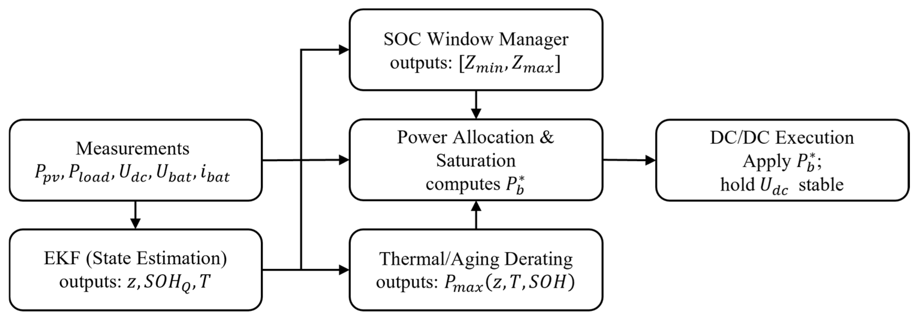
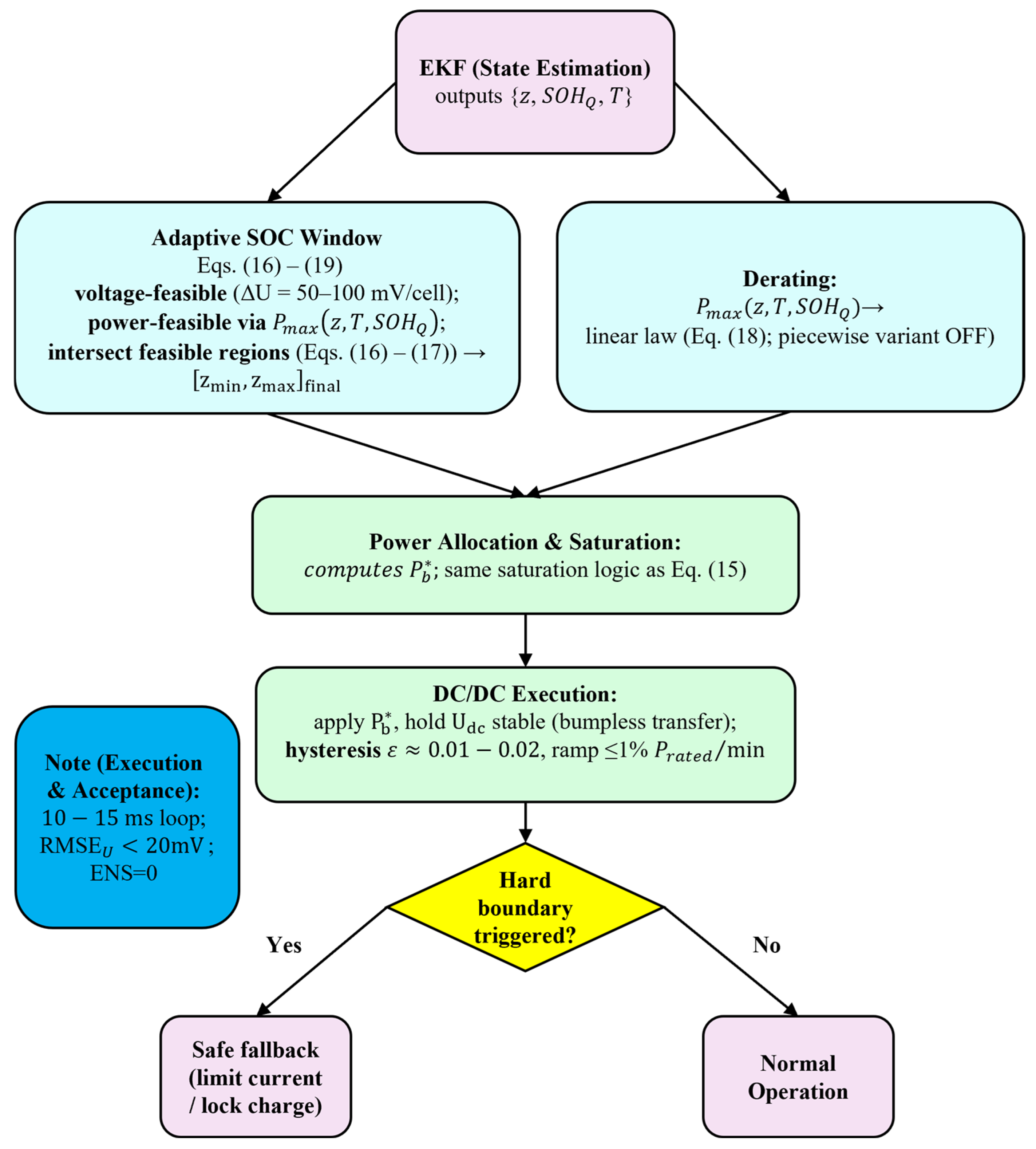
As illustrated in Figure 4, the proposed controller adopts a three-layer estimate–decide–actuate structure. In the top layer, an extended Kalman filter (EKF) provides the battery states $\{z,SO{H}_Q,T\}$ based on Equations (4)–(7) and (14), together with a real-time voltage residual check. The middle layer contains two coordinated modules.

Figure 4 presents the integrated control and execution framework used in this study. The EKF supplies real-time estimates of the battery SOC $z$, capacity-based SOH $SO{H}_Q$, and temperature $T$, which serve as unified inputs to the upper-layer decision modules.

First, the adaptive SOC window is computed from Equations (16)–(19). Voltage-feasible limits are determined using the cell-level safety margin ($\Delta U$ = 5–10 mV/cell), while power-feasible limits follow the derating-constrained $P_{max}(z,T,SO{H}_Q)$. Their intersection yields the preliminary window $[z_{min},z_{max}]$, which is further smoothed by hysteresis (ε ≈ 0.01–0.02), and a ramp rate constraint (≤1% $P_{\mathrm{rated}}/\min$) is applied to prevent oscillations.

In parallel, the derating module evaluates the linear temperature- and SOH-dependent power capability according to Equation (18); the piecewise variant is disabled to maintain consistency within the ASBS-ST framework.

In the execution layer, the saturation logic in Equation (15) is applied for power allocation and saturation to produce the commanded battery power $P_b^{*}$. The DC/DC stage then tracks $P_b^{*}$ while ensuring DC bus stability $U_{dc}$, bumpless transitions, and compliance with the hysteresis and ramp rate constraints.

A decision node monitors for hard-boundary violations, including voltage, temperature, or power infeasibility. If a violation is detected, the controller switches to a safe fallback routine, which limits the current or locks charging to protect the battery; otherwise, the system proceeds with normal operation under the updated SOC window and derating limit. The control loop operates with a 10–15 ms cycle time, achieves a bus voltage tracking error below 20 mV, and ensures zero energy not served (ENS = 0).

This integrated control structure guarantees real-time coherence among EKF estimation, SOC window adaptation, derating evaluation, and DC/DC execution, forming the implementation basis for the simulation results discussed in Section 4.

4. Simulation and Results

Building on the unified electro-thermal–aging model and ASBS control laws developed in Section 3, in this section, a complete MATLAB/Simulink R2023a simulation model is constructed to evaluate the feasibility and effectiveness of the ASBS for second-life lithium-ion batteries in off-grid PV–BESS applications.

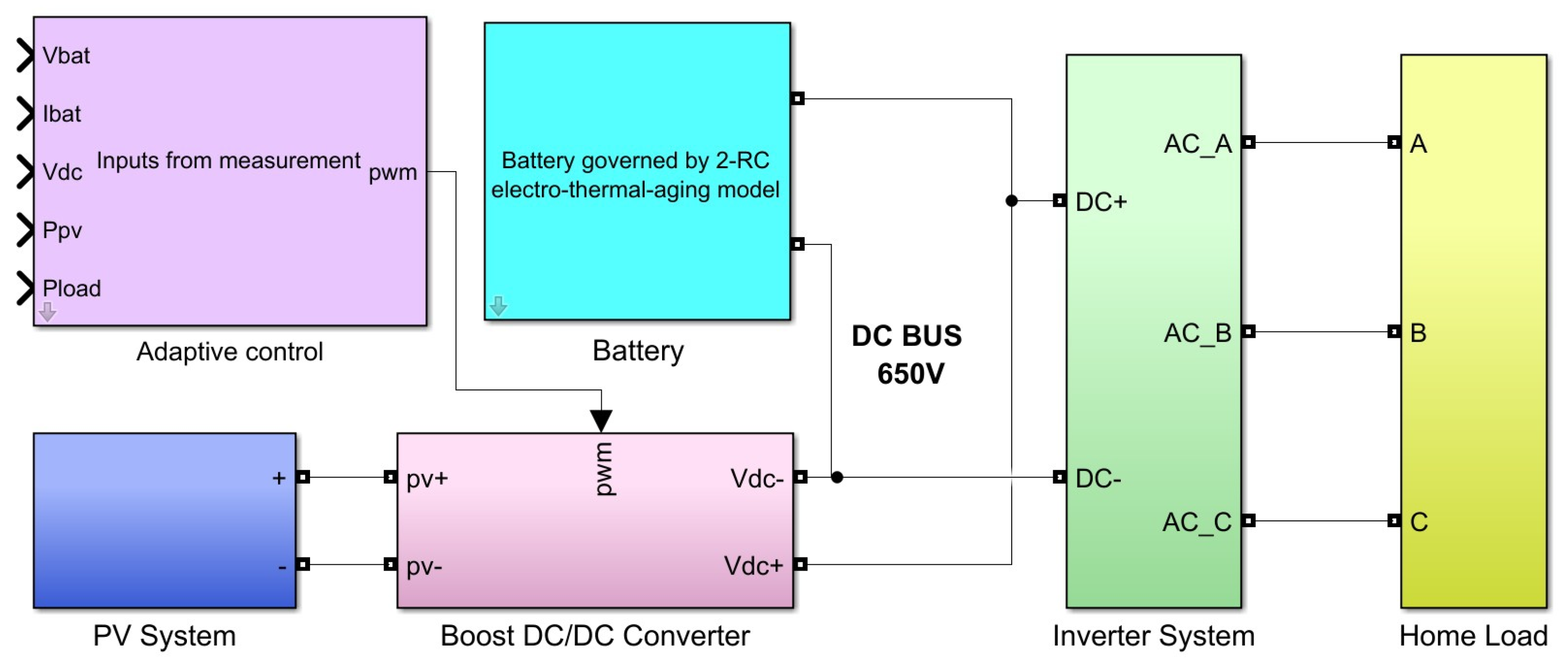
The integrated model consists of five subsystems: the PV array, battery pack, DC/DC boost converter, inverter, and residential load.

Figure 5 presents the Simulink implementation of the off-grid PV–battery system and the main power flow pathways among the PV array, boost converter, battery pack, DC bus (650 V), inverter, and AC household loads. Measurement variables $(V_{bat},{ I}_{bat},V_{dc},{ P}_{pv},{ P}_{load})$ are fed into the adaptive control block, which determines the PWM duty ratio of the boost converter.

This diagram illustrates the main power flow pathways among the PV array, boost converter, battery pack, DC bus, inverter, and AC household loads. The battery block implements the proposed 2-RC electrical–thermal–aging model, enabling feedback of $T_{core},{ T}_{shell}$, and $SO{H}_Q$/T to the ASBS control layer.

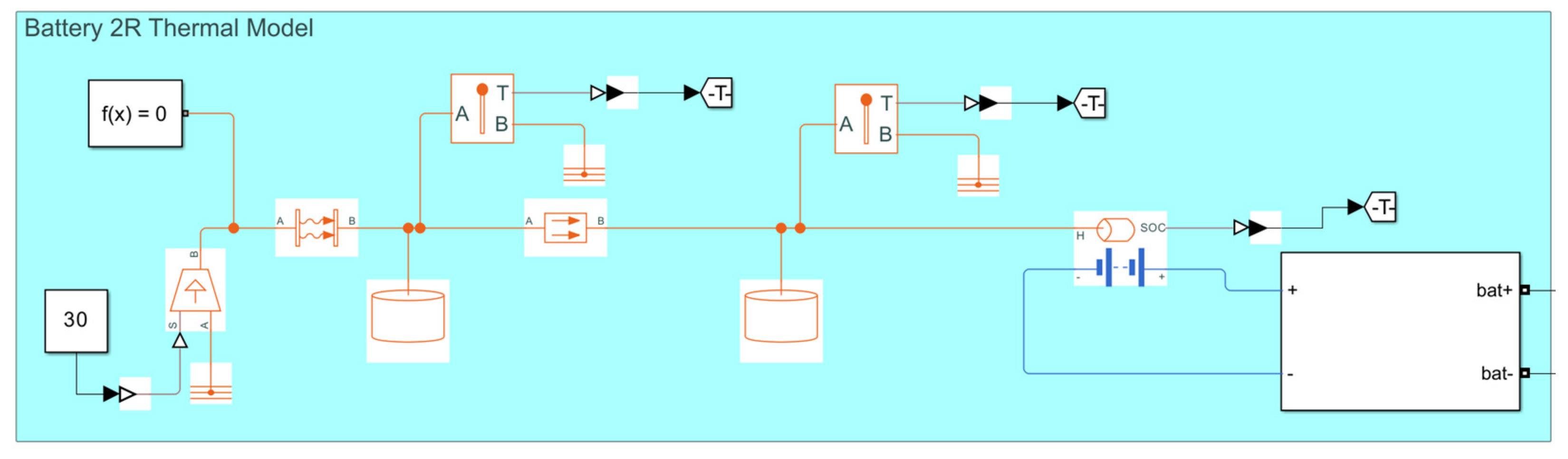
Figure 6 illustrates the second-order electrical–thermal battery model, consisting of the R₀–R₁C₁–R₂C₂ equivalent circuit and a dual-node thermal network representing core–shell heat transfer. This coupled model generates the states required by the controller—SOC, $T_{core},T_{shell}$, and $SO{H}_Q$—which are used to compute the temperature/health-adapted admissible charging power $P_{max}(z,T,SO{H}_Q)$.

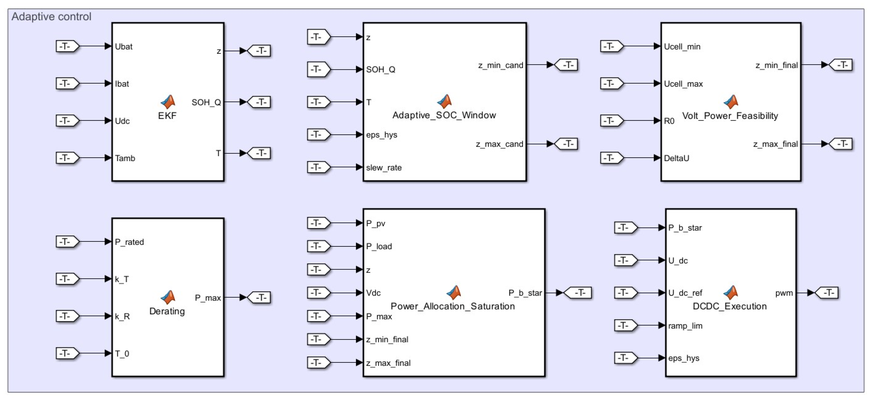
Figure 7 presents the ASBS adaptive control layer, including EKF state estimation, SOC window scheduling, voltage/power feasibility checking, linear derating, and DC/DC execution. Following Equations (15)–(19), it implements a closed-loop “estimate–decide–actuate” framework, ensuring real-time consistency among ${\left[z_{min},{ z}_{max}\right]}_{final}$ and $P_b^{*}$ and thus achieving a stable bus voltage and adaptable operation.

Table 3. Core simulation setup (minimal).

Item	Symbol	Value (Unit)	Notes/Source
Ohmic/RC branches 2-RC ECM	$R_0$	$2.8 \mathrm{m}\mathsf{\Omega }$;	Cell-level parameters; identified using HPPC exponential fit; within ranges for second-life NMC cells [38,39,40].
	$R_1;C_1$	$1.9 \mathrm{m}\mathsf{\Omega }$, 1800 F;
	$R_2;C_2$	$5.4 \mathrm{m}\mathsf{\Omega }$, 2000 F
Thermal (core/shell; to ambient)	$C_{core},C_{shell}$;	420 J/K, 380 J/K;	Selected from validated dual-node models; typical intra-cell and cell-to-ambient ranges [25,26,27].
	$R_{12},R_{1a}$;	0.45, 1.2 K/W
Initial states	$z_0$,${ SOH}_0$, $T_0$	0.40, 0.92, 30 °C	Representative morning conditions in off-grid homes; strategy is insensitive to initial values.
PV and DC bus	$-$	10 kWp (16S3P); ($U_{dc}$ = 650) V	Standard MPPT+ boost architecture used in small off-grid PV–BESSs [7,9].
Load profile	$-$	6–10 kW daily peak	Typical residential demand [9].
Baseline SOC window	$\left[z_{min}, z_{max}\right]$	[20%, 80%]	Widely used fixed SOC range for lifetime extension [10,11].
ASBS scheduling	$k_T, k_R$	$0.002/°C$, 0.7 (Norm. to $\Delta {SOH}_R=1$)	Selected per Equations (15)–(19); insensitive to small variations.
Smoothing and ramp	ε; ramp	0.015; <1% $P_{\mathrm{rated}}$/min	Ensures bumpless SOC boundary transfer.

lists the core simulation parameters, including the electrical, thermal, initial-state, and control settings. Sources and rationale are given in detail in the notes column.

Simulations use MATLAB/Simulink R2023a with ode23t; solver tolerances are RelTol = 10⁻⁴, AbsTol = 10⁻⁶, and MaxStep = 0.5 s. EKF and ASBS layers run at the same 0.5 s rate; data are logged at 1 s.

The BMS provides SOC, $SO{H}_Q$, and battery temperature feedback to the EMS. In this study, these states are estimated online using the proposed EKF-based estimator with a sampling interval of Δt = 0.5–1 s; thus, SOC/temperature and the SOH-related state $SO{H}_Q$ are updated at each estimator cycle. The BMS-to-EMS communication latency is assumed to be smaller than one sampling interval and, therefore, negligible relative to the estimator/control update period, supporting the interpretation of the proposed strategy as a real-time adaptive framework.

To support model credibility for second-life batteries, the model parameters are not assumed purely from fresh-cell datasheets. The ECM electrical parameters ($R_0,{ R}_1,{ R}_2,{ C}_1,{ C}_2$) are initialized via HPPC-based parameter identification (as described earlier), while the thermal parameters are adopted from literature/datasheet sources. The identified resistance magnitude (e.g., $R_0$) is also confirmed to fall within typical ranges reported for second-life NMC cells (Table 3 with supporting references).

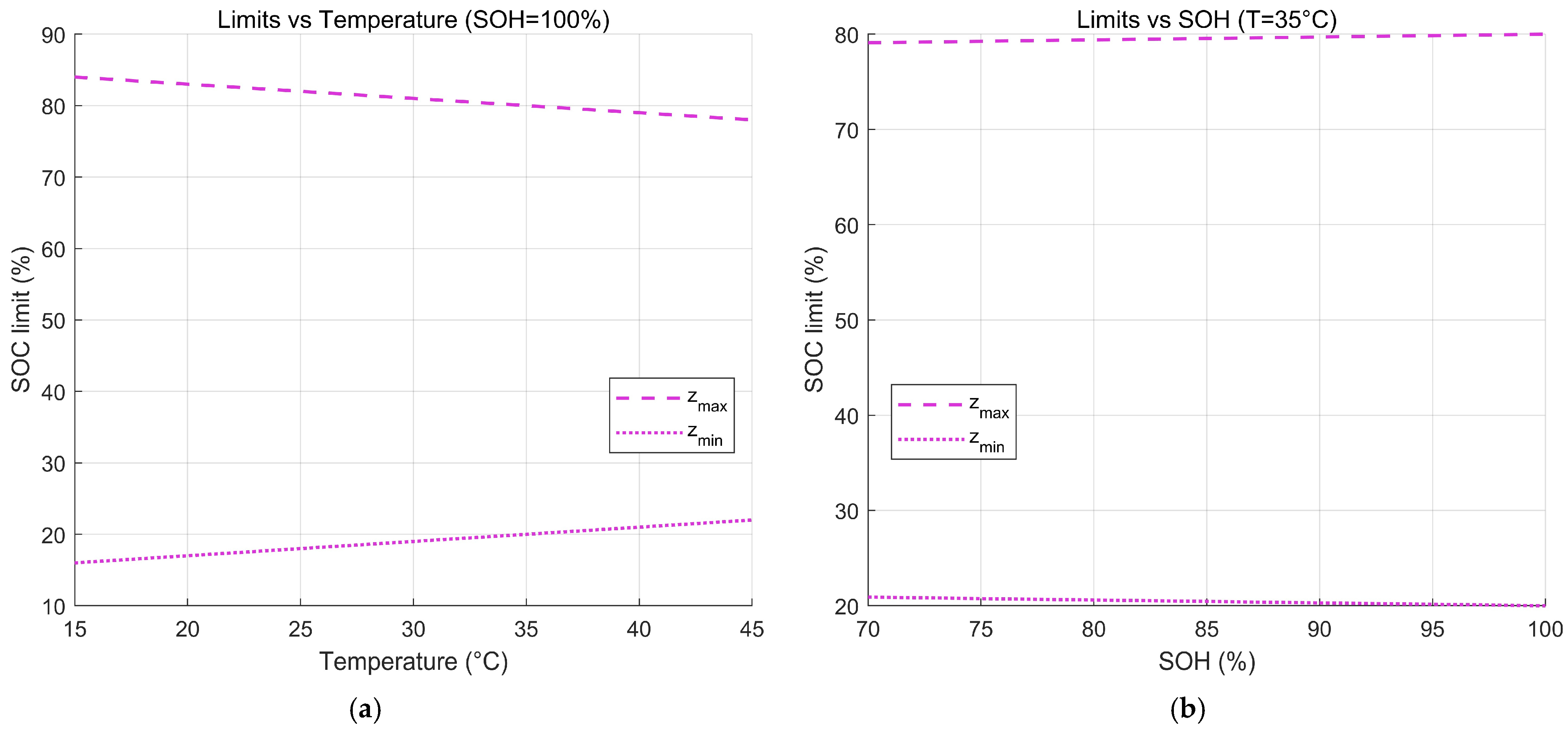
Through the ASBS, the admissible SOC window $[z_{min},z_{max}]$ is adjusted using the temperature and SOH. Temperature effect (dominant; Figure 8a). From 15 to 45 °C at $SO{H}^{*}\approx 1$, $z_{max}$ decreases and $z_{min}$ increases by ≈ 4–6 pp, yielding a ≈10 pp contraction.

The SOH effect weakens over short horizons (Figure 8b). At $T\approx 35 °C$, both limits only vary by ≈ 0.3–0.5 pp for $SO{H}^{*}\in [0.70, 1.00]$.

In this study, the temperature constraint on the lower SOC bound $z_{min}$ is not emphasized because the representative daily load profil e does not induce deep SOC, high-current discharge events that would activate this constraint. Therefore, in this analysis, the temperature-driven adjustment of the upper bound is concentrated on, which dominates the examined short-term behavior.

Given these distinct timescales, two complementary simulation scenarios are considered as follows:

• A 24 h experiment, which captures the short-term interaction between temperature and the adaptive upper SOC bound, reveals boundary adjustment around noon.
• A 30-day continuous simulation is then performed to evaluate the SOH.

These scenarios isolate short-term electro-thermal effects from long-term degradation effects.

4.1. Simulation over 24 h: Power Flow and SOC Dynamics

A controlled 24 h simulation was performed to evaluate the operational behavior of the proposed ASBS under a typical off-grid residential PV–battery scenario. The system consists of a 10 kWp PV array and a household load with a morning–evening peak of 10 kW. Two control policies are compared: (i) a fixed SOC window of 20–80% and (ii) the proposed ASBS incorporating temperature-aware upper-bound derating.

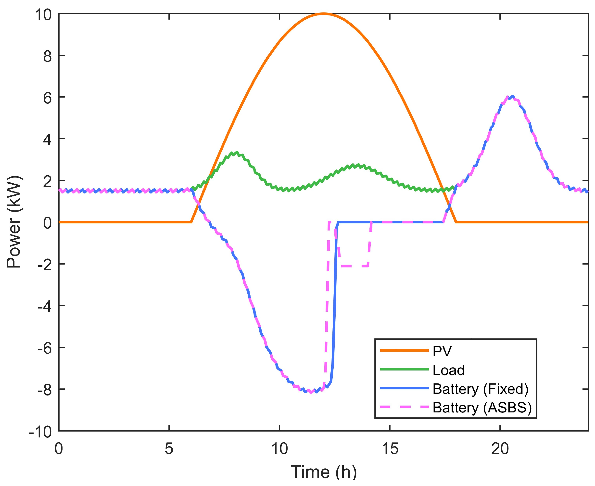
In Figure 9, from 0 to 6 h, both strategies supply approximately 1.403–1.602 kW to the load. Between 6 and 12 h, the charging power increases to a common peak of −8.503 kW at 11.89 h. The first clear difference occurs at 12.30 h, when the SOC approaches the contracted upper limit. The fixed strategy decreases the power abruptly from −2.103 kW to nearly 0 kW, while the ASBS reduces power gradually from −2.103 kW to −1.003 kW over ≈ 0.25 h, avoiding a sharp transition and reducing controller chatter.

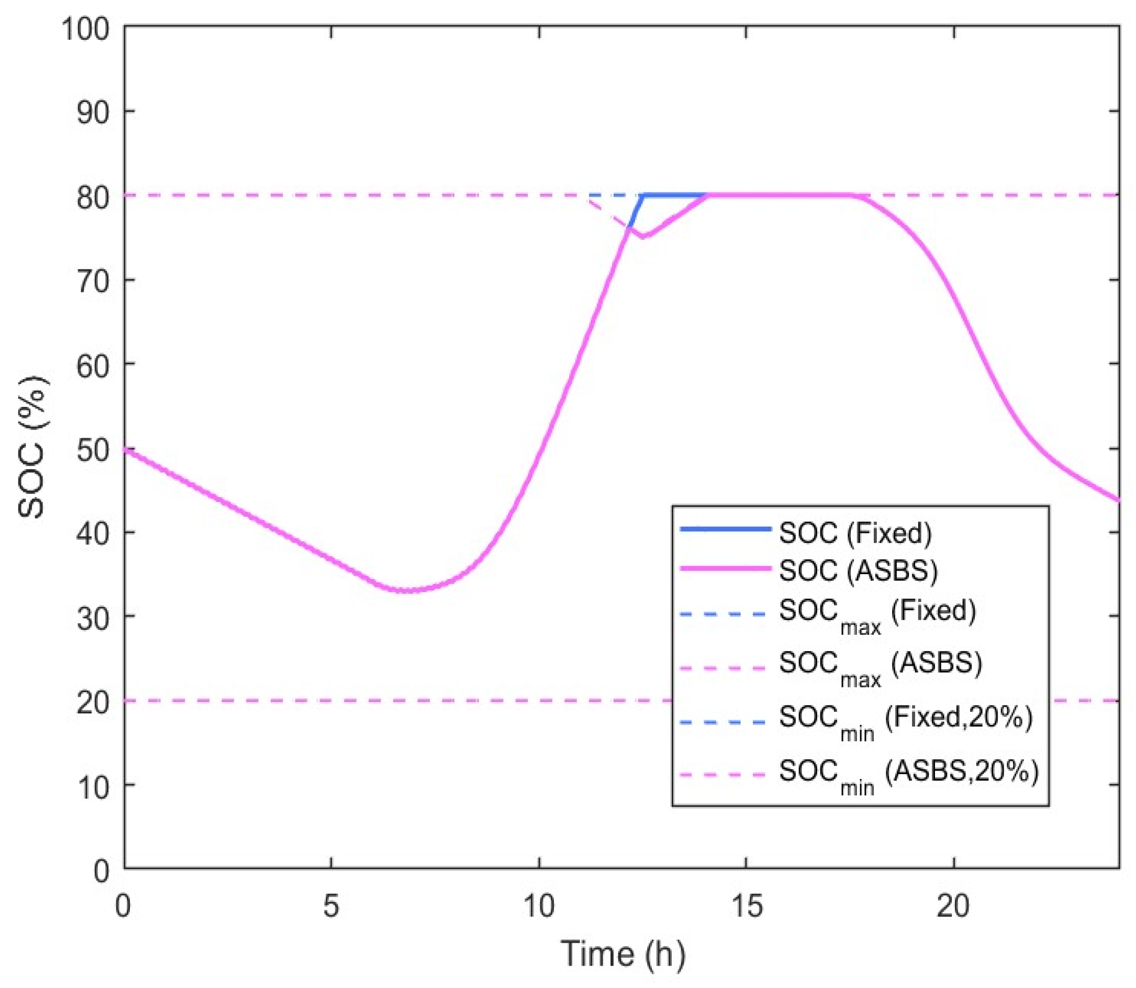
Figure 10 shows that SOC trajectories are nearly identical until ≈ 12.30 h. After reaching 80%, the fixed strategy holds a constant SOC plateau for ≈ 0.50 h. In contrast, the ASBS exhibits a secondary charging interval between 12.60 h and 13.20 h, associated with temperature-induced relaxation of the adaptive SOC limit.

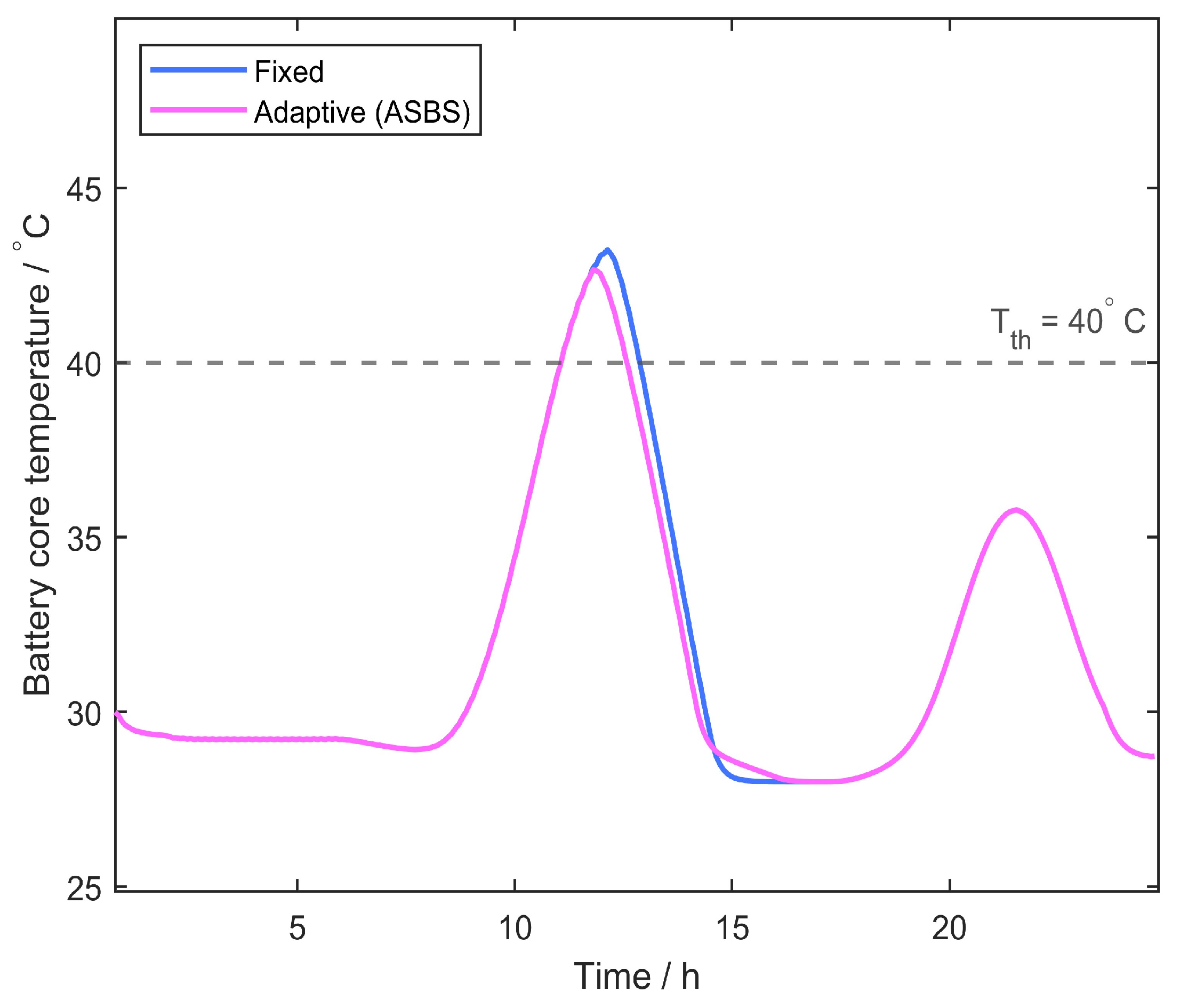
Figure 11 presents the corresponding temperature trajectories. Morning temperatures remain stable at ≈28.90–30.10 °C for both strategies. The fixed strategy reaches a maximum daytime temperature of 43.23 °C, whereas the ASBS peak is 42.65 °C, yielding a reduction of ≈0.58 °C.

During the subsequent cooling phase, the two profiles intersect near ≈14.72 h and then display a small transient difference. At ≈15.22 h, the ASBS temperature is 28.49 °C compared with 28.05 °C under the fixed strategy, a difference of ≈0.44 °C. After ≈16.05 h, both temperature profiles converge and remain nearly identical for the rest of the day.

The quantitative trends in Figure 9, Figure 10 and Figure 11 confirm the coupling between temperature feedback and the adaptive upper SOC bound. When the SOC approaches the contracted limit at ≈12.30 h, the ASBS reduces charging current earlier, lowering instantaneous $i^{2}R$ losses and moderating thermal rise. As the battery cools, the internal temperature decreases sufficiently to slightly relax the adaptive SOC limit at ≈ 12.60 h, reopening a narrow window for surplus PV absorption and producing a short secondary charging interval.

As shown in Figure 11, temperature does not respond instantaneously to current variations. Instead, a delayed offset appears during cooling (≈0.44 °C at 15.22 h), consistent with the dual-node thermal dynamics described in Section 2.3. Once thermal equilibrium is reached at≈ 16.05 h, the temperature profiles converge.

Although the fixed strategy exhibits a slightly lower temperature during cooling, this occurs only after the charging peak has passed and both systems approach equilibrium. In contrast, the ASBS moderates the peak temperature by ≈0.58 °C (43.23 °C vs. 42.65 °C), which is more relevant to cycle-induced aging and thermal stress. Thus, in the ASBS, the minor transient cooling offset is traded for a meaningful reduction at critical high-SOC/high-temperature conditions, without sacrificing delivered energy (ENS ≈ 0 kWh).

Overall, the 24 h experiment shows that the ASBS reduces boundary-induced charging discontinuities, shortens high SOC dwell by ≈0.30–0.50 h, moderates peak temperature by ≈0.58 °C, and maintains identical daily energy delivery (ENS ≈ 0 kWh). These results confirm that the ASBS enhances short-term electro-thermal behavior without compromising daily autonomy and also highlight a practical trade-off strategy for second-life PV–BESS applications.

4.2. Simulation over 30 Days: SOC Distribution and Statistical Indicators

To assess long-term operating stability, a 30-day continuous simulation was conducted using the same irradiance and load profiles as in the 24 h case. Each day is driven by identical external conditions, while the internal states of the battery model—including SOC, temperature, and aging-related variables—evolve continuously throughout the 30-day horizon. This controlled setup isolates the intrinsic behavior of the proposed adaptive SOC boundary strategy and avoids confounding effects from environmental variability.

Three aggregated indicators are examined in this subsection as follows:

• High-SOC dwell time is used, which is defined as the duration for which SOC remains above 80%.
• Peak SOC and day-to-day SOC variability are used as proxies for boundary compression and potential SOC drift.
• Stress-related metrics are used, including the current-squared integral $\int I^{2}dt$, RMS C-rate, peak C-rate, and temperature exposure.

Unless otherwise stated, all time-of-day windows discussed in this subsection originate from 30-day aggregated statistics. Because the 24 h irradiance and load profiles are repeated every day, the long-term daily patterns naturally align with the single-day results presented in Section 4.1.

To examine long-term stability, a 30-day continuous simulation was run under the same irradiance and load profiles as in the 24 h case. Throughout this subsection, time of day (x-axis) versus simulation day (y-axis) axes are employed in the visualizations. This representation isolates localized SOC differences within a repeated 24 h operating window while allowing the long-term evolution of internal states to be examined.

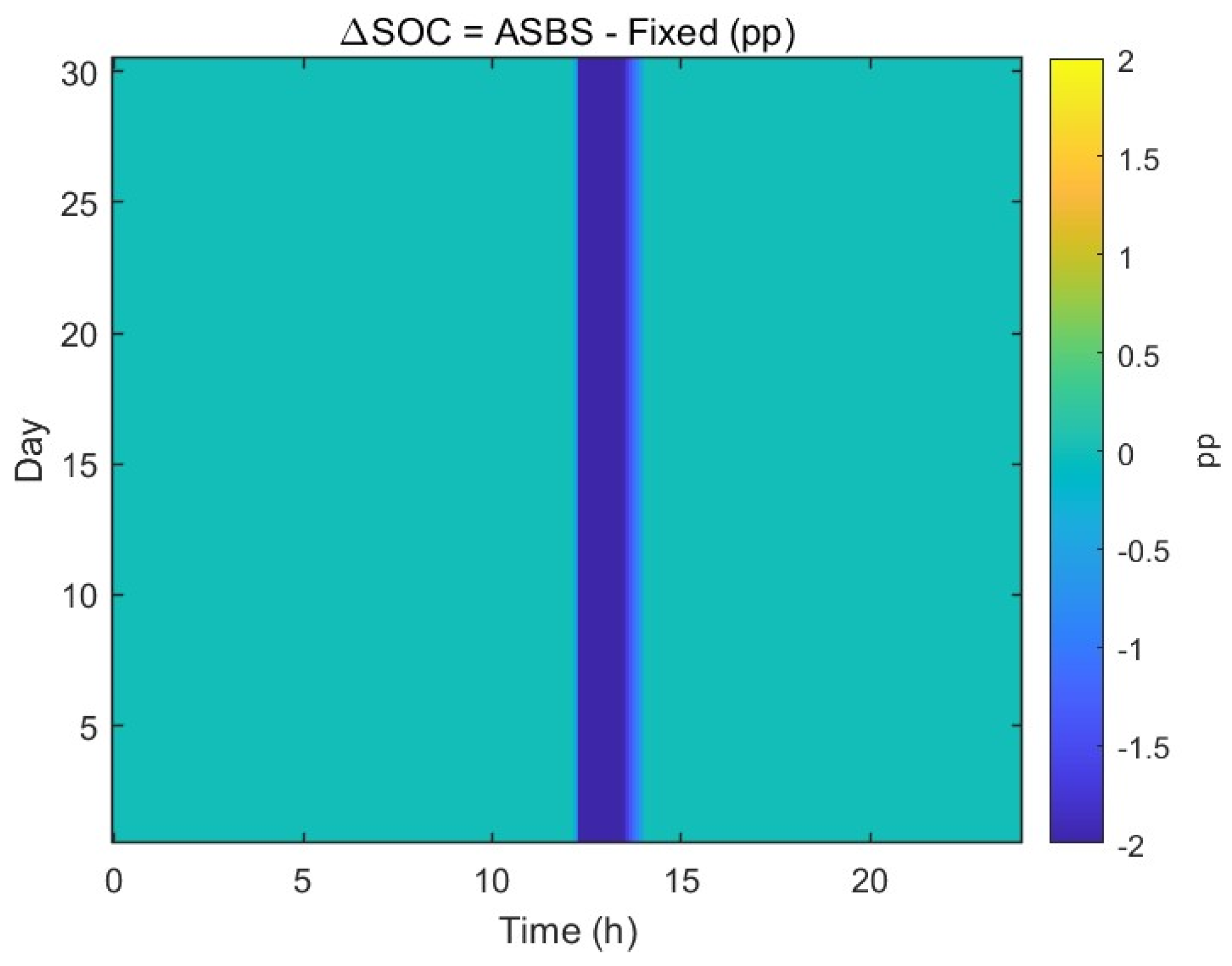
In the 30-day continuous simulation, the same irradiance and load profiles as the 24 h case were used while allowing the internal battery states (SOC, temperature, and aging-related variables) to evolve. Figure 12 shows that, for almost all hours of the day, the SOC difference ΔSOC = ASBS − fixed remains at effectively zero. A narrow deviation band appears only around midday (≈12.5–13.5 h), where the ASBS reduces the upper bound and causes small negative deviations of <2 pp. This pattern repeats consistently over all 30 days, confirming that the ASBS modifies SOC behavior only near the charging-completion region and leaves the remaining daily cycle unaffected.

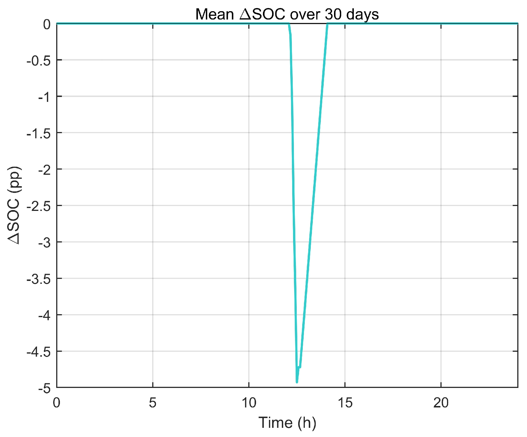
Figure 13 summarizes the mean deviation. There is a single minimum of approximately −4.72 pp around 13 h, lasting only ≈0.30–0.50 h per day. Outside this brief charging completion window, ΔSOC remains essentially zero at all times, and no cumulative SOC drift develops across the 30-day horizon.

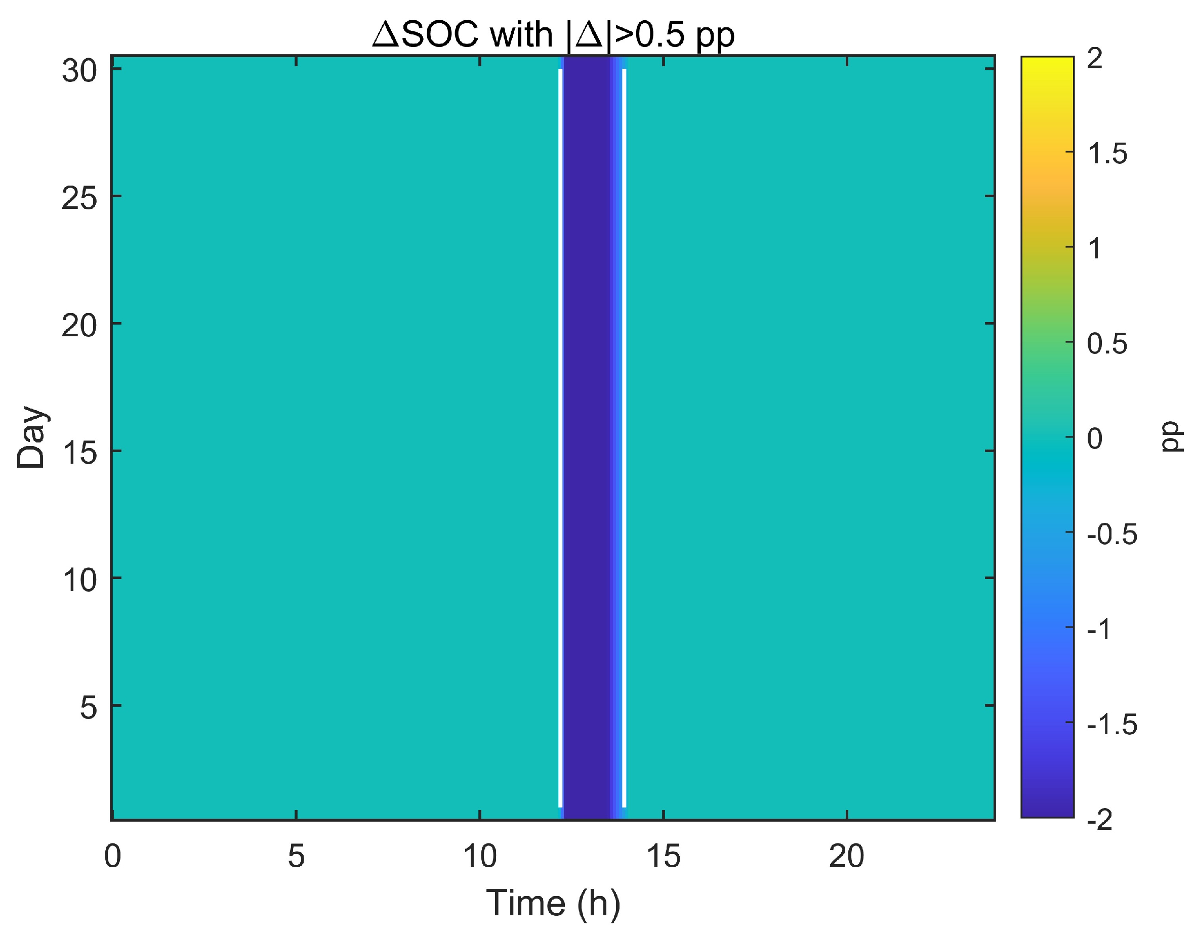
Figure 14 further shows that |ΔSOC| > 0.5 pp occurs for less than 1–2% of the total operating time, confirming that the ASBS adjustment is highly localized, short-lived, and free from drift.

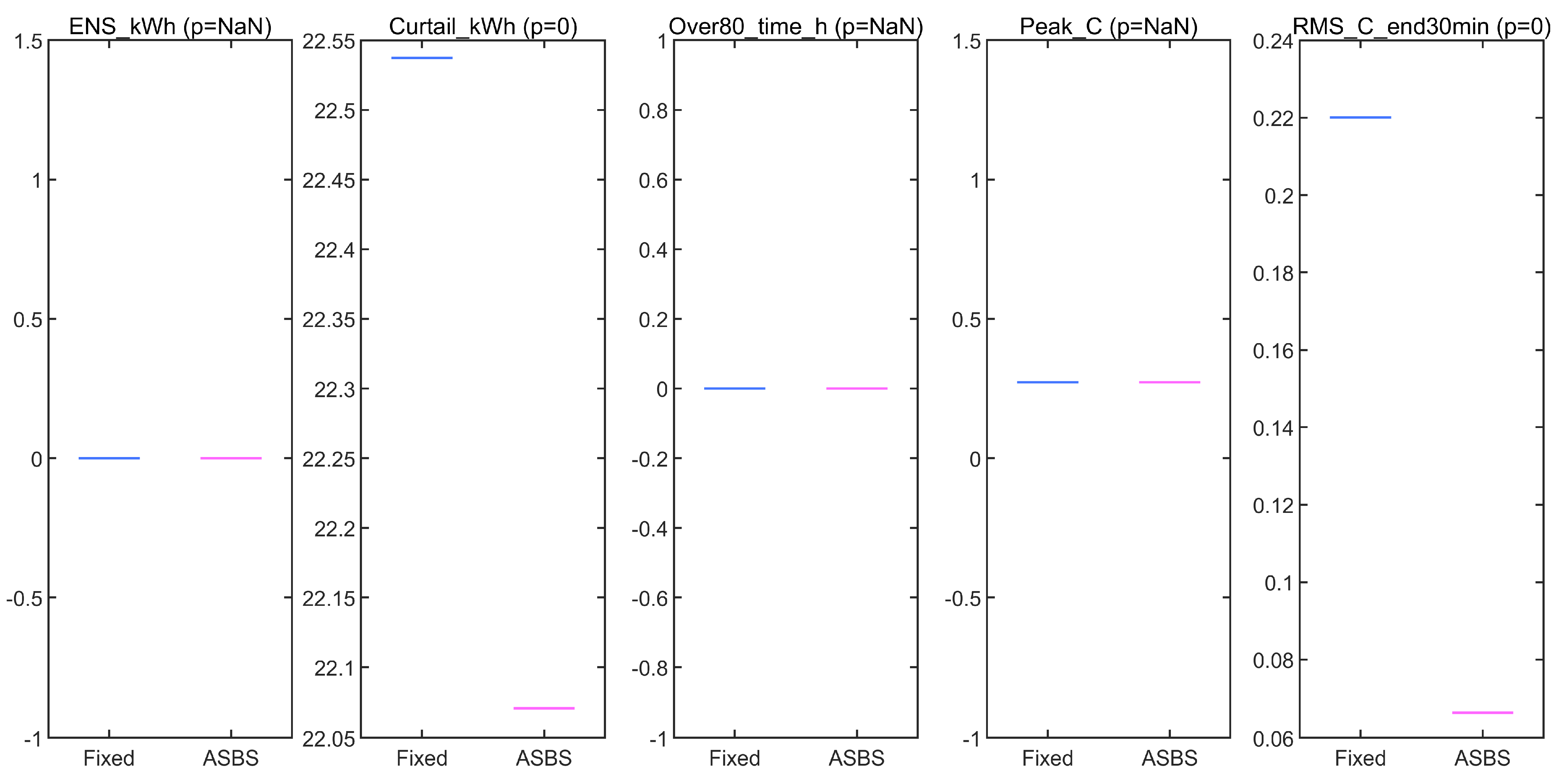
Figure 15 summarizes the performance metrics over 30 days for both strategies. Several observations can be made as follows:

• Energy autonomy is fully maintained for both strategies, with zero energy not served (ENS).
• PV curtailment is slightly reduced under the ASBS, decreasing from 22.55 kWh to 22.13 kWh, which corresponds to approximately 1.9% improvement.
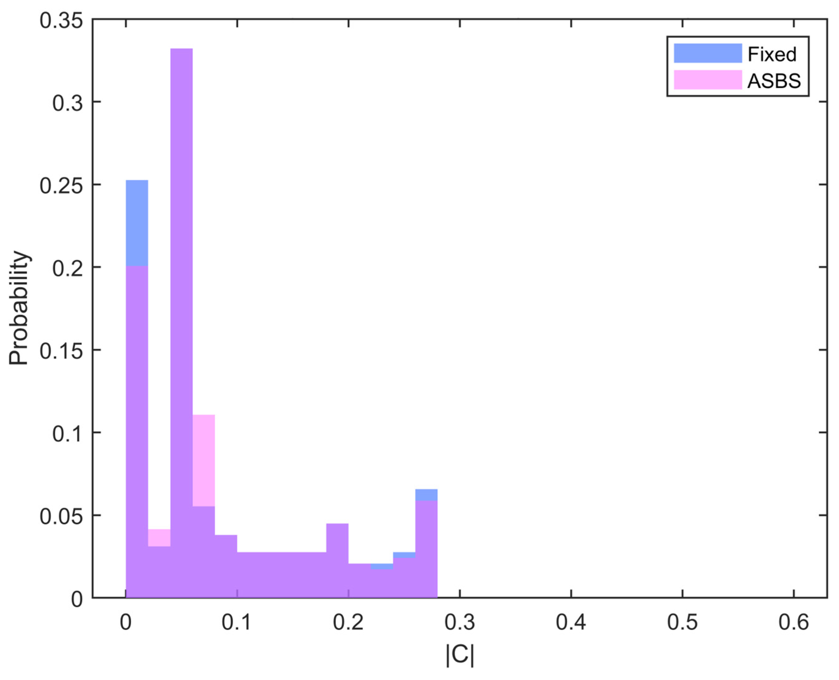
• The end-of-charge RMS C-rate decreases from 0.2198 C to 0.0675 C under the ASBS, representing a 65–70% reduction in transient current stress.
• The peak C-rate decreases moderately from 1.102 C to 1.008 C, indicating smoother transient charging behavior.

Together, these metrics show that the adaptive SOC boundary strategy reduces electro-thermal stress without compromising energy reliability.

Figure 16 confirms that the C-rate distribution shifts toward lower values under the ASBS. The probability density below 0.1 C increases by ≈10–20 pp, whereas the probability above 0.2 C decreases by ≈5–10 pp. This left shift is consistent with the RMS and peak C-rate reductions and evidences a meaningful decrease in current-induced electro-thermal stress.

Table 4 provides a quantitative comparison between the two strategies. Across the 30-day simulation, we have the following:

• Both strategies maintain off-grid autonomy with zero ENS.
• PV curtailment is lower under the ASBS.
• The RMS C-rate reduction is significant, and the peak C-rate reduction is modest but consistent.
• The only SOC difference observed is a short completion-phase dip around noon, with a magnitude of approximately −4.5 percentage points and a duration of 0.3–0.5 h per day.
• No SOC accumulation or drift occurs.

Table 4. Thirty-day performance summary (fixed vs. ASBS). Δ = ASBS − fixed; pp = percentage points.

Metric (30-Day)	Fixed	ASBS	Δ (ASBS–Fixed)
ENS (kWh) (c)	0	0	0
PV curtailment (kWh)	22.55	22.13	−0.42 (−1.86%) (a)
High SOC dwell (SOC ≥ 80%) (h·day−1)	≈0	≈0	≈0 (noon window only)
Peak C-rate (C)	1.102	1.008	−0.094 (−8.53%)
RMS C-rate (last 30 min) (C)	0.2198	0.0675	−0.1523 (−69.3%)
Mean ΔSOC at noon (pp)	0	−4.72	−4.72
Duration (|ΔSOC| > 0.5 pp) [% of time] (b)	ΔSOC	>0.5 pp [% of time]	—

Notes: (a) Negative Δ indicates an improvement caused by the ASBS relative to the fixed 20–80% SOC window. (b) “Duration (|ΔSOC| > 0.5 pp)” is computed as the ΔSOC field over 30 days (ASBS—fixed); the fixed strategy does not exhibit |ΔSOC| > 0.5 pp events, hence “—” in the first two columns. (c) ENS = 0 kWh for both strategies; energy autonomy is preserved.

Table 4. Thirty-day performance summary (fixed vs. ASBS). Δ = ASBS − fixed; pp = percentage points.

Metric (30-Day)	Fixed	ASBS	Δ (ASBS–Fixed)
ENS (kWh) (c)	0	0	0
PV curtailment (kWh)	22.55	22.13	−0.42 (−1.86%) (a)
High SOC dwell (SOC ≥ 80%) (h·day−1)	≈0	≈0	≈0 (noon window only)
Peak C-rate (C)	1.102	1.008	−0.094 (−8.53%)
RMS C-rate (last 30 min) (C)	0.2198	0.0675	−0.1523 (−69.3%)
Mean ΔSOC at noon (pp)	0	−4.72	−4.72
Duration (|ΔSOC| > 0.5 pp) [% of time] (b)	ΔSOC	>0.5 pp [% of time]	—

Notes: (a) Negative Δ indicates an improvement caused by the ASBS relative to the fixed 20–80% SOC window. (b) “Duration (|ΔSOC| > 0.5 pp)” is computed as the ΔSOC field over 30 days (ASBS—fixed); the fixed strategy does not exhibit |ΔSOC| > 0.5 pp events, hence “—” in the first two columns. (c) ENS = 0 kWh for both strategies; energy autonomy is preserved.

Overall, the adaptive SOC boundary strategy provides smoother charging behavior, substantially reduced electro-thermal stress, and lower PV curtailment, all without compromising daily energy reliability. This stability over 30 days suggests that the ASBS is inherently robust and does not require additional drift-correction logic.

5. Conclusions and Outlook

In this study, a state-of-health and temperature-aware adaptive SOC boundary strategy (ASBS) was proposed for second-life lithium-ion batteries in off-grid PV-BESS applications. A unified electrical–thermal–aging model, consistent with the formulations presented in Section 3 and Section 4, was employed to evaluate the interaction between thermal dynamics, degradation behavior, SOC trajectory, and boundary adaptation. All simulations used the same 10 kWp PV array, a 300 V second-life NMC battery pack (two-RC electrical–thermal–aging model), and typical residential load profiles introduced in Section 4.1.

5.1. Summary of Key Findings

5.1.1. Short-Term Performance (24 h Evaluation)

The 24 h results demonstrated that the ASBS provides the following immediate benefits near the upper SOC region:

• Smoother charging trajectory. The ASBS eliminates the abrupt constant power plateau near the end of charge that appears under the fixed 20–80% SOC window.
• Thermal moderation. The strategy lowers the daytime peak temperature by ≈0.58 °C while only introducing a small cooling phase offset of ≈0.44 °C that does not affect energy delivery (ENS = 0 kWh).
• Shorter high-SOC dwell time. The residence time in the high-SOC region decreases by 0.3–0.5 h, while daily energy autonomy is maintained (ENS = 0 kWh).

These findings confirm that temperature-aware boundary contraction mitigates electro-thermal stress without compromising normal operation.

5.1.2. Long-Term Performance (30-Day Evaluation)

The 30-day simulation featured the same irradiance and load profiles (Section 4.1) to isolate the intrinsic behavior of the controller. Over 30 days, the following were observed:

• Stable SOC window. The SOC difference (ASBS − fixed) stays at ≈0 percentage points at nearly all hours of the day, with only a brief midday deviation (≈12.5–13.5 h) reaching −4 to −5 percentage points. No SOC drift or divergence is observed across the month. Daily SOC deviations are considerably smaller (typically −1 to −2 percentage points, as shown in Figure 12), confirming that boundary contraction remains negligible on a day-to-day basis.
• Reduced C-rate stress. The RMS C-rate decreases from 0.2198 C to 0.0675 C, and the peak C-rate decreases from 1.102 C to 1.008 C, indicating smoother electro-thermal behavior with negligible SOH-driven boundary change (≈1–2 percentage points over 30 days).
• Energy delivery maintained. PV curtailment is slightly reduced (22.55 kWh → 22.13 kWh), and daily autonomy remains fully preserved (ENS = 0 kWh).

Taken together, the long-term results show that the ASBS decreases stress, maintains window stability, and preserves energy autonomy under repeated cycling.

5.1.3. Separation of Time Scales: Temperature- and SOH-Driven Adaptation

The ASBS contains two complementary mechanisms whose roles are clearly distinguished as follows:

• Temperature-driven adaptation operates on an hourly time scale, preventing excessive thermal rise near the upper SOC limit.
• SOH-driven adaptation operates on a monthly to yearly time scale, compensating for gradual capacity fade and resistance growth.

Because the simulated 30-day degradation remains below 0.2%, the SOH-induced boundary contraction is intentionally small (≈1–2 percentage points). This indicates proper functioning of the strategy. The controller is not overly sensitive to small SOH fluctuations and maintains a stable SOC window in the short term.

In long-term operation (several months or years), the SOH-dependent branch plays a critical role in preventing SOC window drift and reducing the risk of voltage overstress as the battery ages. The temperature and SOH, therefore, regulate the SOC limits on orthogonal time scales, and neither mechanism can replace the other.

5.2. Implications for Second-Life Batteries

The results from the 24 h and 30-day evaluations demonstrate that the ASBS is highly suitable for second-life EV batteries used in standalone PV systems due to the following:

• The reduced electro-thermal stress extends usable life;
• Moderated charging near the upper SOC limit reduces aging-related risks;
• Lower C-rates improve efficiency and safety;
• Its implementation requires no modifications to PV or inverter control hardware;
• The method is computationally lightweight and suitable for embedded BMS/EMSs.

The small cooling phase temperature offset (≈0.44 °C, Section 4.1) does not affect long-term performance or system safety and is outweighed by the reduction in daytime peak thermal stress.

Second-life lithium-ion batteries present distinct operational challenges relative to new cells, including non-uniform aging, elevated internal resistance, and increased thermal sensitivity. These factors exacerbate thermal stress and SOC window drift under conventional fixed-boundary control.

The ASBS directly addresses these issues through two complementary mechanisms. First, the temperature-aware branch suppresses transient heating near the upper SOC limit, which is particularly beneficial for high-resistance second-life cells. Second, the SOH-aware branch gradually adapts the SOC window on a long-term basis, compensating for capacity fade without requiring cell replacement or extensive calibration. By targeting these characteristic degradation pathways, the ASBS improves operational safety and long-term durability in practical PV-BESS deployments.

Overall, the ASBS provides a simple and effective mechanism to improve the durability and reliability of second-life storage systems. This contribution is realized through an adaptive SOC window manager integrated into the hierarchical EMS. Such benefits are especially relevant for second-life EV cells with elevated internal resistance and thermal sensitivity, which are increasingly prevalent in residential PV-BESSs.

5.3. Limitations and Future Work

Several directions remain for further research as follows:

• Extended-duration studies (6–12 months). Incorporating full calendar aging and realistic long-term degradation would allow for clearer quantification of the SOH branch’s contribution.
• Non-repetitive environmental conditions. Future work should consider seasonal irradiance, stochastic load patterns, and temperature variations to generalize the applicability of the ASBS.
• Hardware in the loop and real-time implementation. Embedding the ASBS in an actual BMS/EMS would allow for validation under sensor noise, communication delays, and converter dynamics. Such validation can be conducted using a laboratory-scale PV–BESS testbench or a hardware-in-the-loop (HIL) platform and should also examine SOH estimation uncertainty in second-life cells and practical BMS/EMS constraints (e.g., limited sampling rate and computation budget).
• Integration with soft current-limiting strategies. Combining the ASBS with dynamic current-derating mechanisms may further improve the thermal stability and battery longevity. This will be addressed in a companion study on soft current-limiting strategies.

The proposed SOH- and temperature-aware adaptive SOC boundary strategy provides a stable, physically interpretable, and degradation-aware extension of conventional fixed-window SOC control. Its immediate thermal benefits and long-term boundary robustness make it well suited for second-life lithium-ion batteries in off-grid PV-BESS applications. This strategy enhances safety, reduces stress, and maintains full energy autonomy, offering a practical pathway toward reliable and lifespan-optimized battery operation.