Abstract
Shift organizations in automotive manufacturing often rely on manual task allocation, resulting in inefficiencies, human error, and increased workload for supervisors. This research introduces an automated solution using the Kuhn-Munkres algorithm, integrated with the Moodle learning management system, to optimize task assignments based on operator qualifications and task complexity. Simulations conducted with real industrial data demonstrate that the proposed method meets operational requirements, both logically and mathematically. The system improves the start of shifts by assigning simpler tasks initially, enhancing operator confidence and reducing the need for assistance. It also ensures that task assignments align with required training levels, improving quality and process reliability. For industrial practitioners, the approach provides a practical tool to reduce planning time, human error, and supervisory burden, while increasing shift productivity. From an academic perspective, the study contributes to applied operations research and workforce optimization, offering a replicable model grounded in real-world applications. The integration of algorithmic task allocation with training systems enables a more accurate matching of workforce capabilities to production demands. This study aims to support data-driven decision-making in shift management, with the potential to enhance operational efficiency and encourage timely start of work, thereby possibly contributing to smoother production flow and improved organizational performance.
1. Introduction
In industrial environments where human resources play a direct role in product manufacturing (e.g., manual assembly), the optimal and compliant allocation of operators is a common challenge [1,2]. In the study “Notification Timing for On-Demand Personnel Scheduling,” the authors propose a system that assigns shifts for casual or temporary jobs to workers. The system ranks casual employees based on seniority and notifies them about available job opportunities. Their solution results in better job–worker matches compared to the method used by their industry partner. However, the downside is that lower-seniority employees may be excluded, limiting their opportunities for growth. Furthermore, the algorithm can only handle one-day schedules [3].
Heuristic algorithms can be enhanced with neural networks. In the study “Apply Artificial Neural Network to Solving Manpower Scheduling Problem,” the authors developed a scheduling generation algorithm that first creates initial schedules using a genetic algorithm, and then a neural network (Feedforward Deep Neural Network) learns to optimize them. This is an effective solution, as it considers the company’s manufacturing requirements and is capable of planning long-term schedules in advance. However, due to the neural network training, the solution is resource-intensive and may have high initial implementation costs [4].
At our industry partner, the goal of initiating shift scheduling is to represent an innovative and sustainable solution that can have a direct and positive impact on production efficiency by considering operators’ capabilities while not ignoring their weaknesses. The implementation cost should be kept as low as possible, and the operation of the system should not require specialized knowledge.
Moreover, it is critical that every operator adheres to the same standards and procedures. Learning Management Systems (LMSs) play a key role in supporting manufacturing processes [5] by providing an efficient training platform for employees [6]. LMSs support the continuous training and knowledge updates of staff, which is particularly important in complex manufacturing processes where the rapid advancement of new technologies and procedures requires constant adaptation. The system also enables tracking and analysis of training outcomes.
The Moodle is an open-source platform-based LMS [7], which is highly flexible due to its modular structure, allowing customization with various modules and plugins [8]. In a LAMP (Linux, Apache, MySQL, PHP) environment, it can be easily extended to meet fully customized requirements [9], making it entirely adaptable to the needs of a manufacturing company.
Our goal is to assign operators to production tasks based on specific production characteristics [10]. The Kuhn-Munkres algorithm, also known as the Hungarian algorithm, is used for cost-based optimal assignment problems. The algorithm is rooted in the research work of Hungarian mathematicians Dénes Kőnig and Jenő Egerváry, which is the origin of its name [11]. A key requirement of the algorithm is the use of an n × n matrix, where, in our case, the rows represent operators and the columns represent products. The cells represent efficiency values, indicating how well an operator performs in each production process.
The steps of the algorithm (working principles) are as follows:
- Subtract the smallest element in each row from all elements in that row.
- Subtract the smallest element in each column from all elements in that column.
- Draw lines over rows and columns to cover all zeros in the matrix using the minimum number of possible lines.
- The stopping condition is met if the number of lines equals the number of rows in the matrix.
- If the stopping condition (step 4) is not met, find the smallest uncovered element. Subtract it from all uncovered elements and add it to every element covered by two lines. Then, repeat step 3.
- Repeat the cycle until the stopping condition is met. At this point, select a subset where each row and column contain only one chosen zero. Then, remove any dummy rows/columns that were previously added. The zeros in the final matrix represent the optimal assignment in the original matrix. These indicate which task is assigned to which worker in the ideal distribution [12].
The algorithm was applied in conjunction with the Moodle Learning Management System to address the complex problem of workforce allocation at an automotive company. For large workforce sizes, this process can be time-consuming, costing the company valuable minutes of production time. At the same time, adhering to complex manufacturing regulations demands significant attention and energy from the administrative staff. Administrators must account for operators’ work efficiency, individual characteristics, preferences, and the required training for specific product manufacturing. This can create stress during their work, potentially leading to serious errors.
Our goal is to enhance efficiency and reduce the uncertainty and stress often experienced at the beginning of shifts through automated workforce allocation.
2. Related Works
The assignment problem is present in most industrial domains. In the study by Bai, X [13], a transportation task was solved through optimization. The goal was to ensure that transportation vehicles with specific characteristics (aerial/marine) delivered the cargo to the appropriate destination via the shortest possible route. In addition to route planning, they also had to solve the problem of assigning target points to the respective vehicles. Considering safety requirements, they defined a sufficient set of conditions. To assign targets to vehicles, they applied a complex genetic algorithm that combines virtual coding (to describe routes and assignments), multiple offspring generation, inter-population crossover (referred to as “intermarriage crossover”), and the tabu search mechanism. The new algorithm proved to be more efficient compared to greedy algorithms.
In the study “Distributed Multi-Vehicle Task Assignment in a Time-Invariant Drift Field with Obstacles”, a near-optimal solution was found for an NP-complete problem using a task assignment method [14]. Target locations were assigned to different vehicles. A path-planning method was developed that enables a vehicle to travel between two points in the shortest possible time while avoiding obstacles. The optimization was carried out in two steps using the new method: first, a cost matrix was generated based on time-minimizing path planning, and then, an auction-based distributed algorithm was used to assign tasks to the vehicles.
Data-driven decision-making is also highly applicable in the field of tourism [15]. In a survey, 2400 tourists were asked about their international travel experiences. Based on the collected data, machine learning models were developed and evaluated using metrics such as accuracy, precision, recall, F-score, and ROC curve. The proposed model in the study first generates categorized recommendations, which are then refined by a personalized algorithm through weighted decision-making to determine the final recommended destinations. According to the results, the proposed system provides more accurate and efficient recommendations than existing systems.
Wind power performance, long utilized in the energy sector, can also be effectively optimized using appropriate configuration and assignment algorithms [16]. The study addressed a task within a wind farm composed of wind turbines and substations. A method was developed to minimize both infrastructure costs and energy losses. The approach involves dividing the group of turbines into subgroups and assigning them to corresponding parcels using a combination of genetic algorithms (GAs) and integer linear programming (ILP). With this optimized method, a cost saving of 0.17% was achieved compared to traditional (non-optimized) clustering approaches.
3. Methods
The injection molding of polymer parts and their assembly take place in a continuous production schedule (24/7) for 360 days a year at an automotive company. The company produces 1.5 million parts daily, which are assembled and packaged by 50–80 operators. The solution related to the operators’ daily schedule must begin with gathering relevant information. Based on the organizational structure, the departments involved in scheduling were identified (marked in red in Figure 1). The relevant managers for this process were also identified. The list of stakeholders was expanded to include the employees performing the work as well.
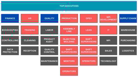
Figure 1.
Organizational units and their involvement.
The information necessary for starting the shifts was collected during the internal interviews. One of the most important interviews was with the production manager, where it was confirmed that efficient task allocation for operators at the start of shifts is necessary.
The technical descriptions, standards, internal company documents, regulations, and work instructions related to this problem were reviewed and organized. Based on this, one of the key points is the administrative processes changing. Additionally, a set of requirements were created, which defines the needs related to the efficient task allocation.
The problems and requirements are as follows:
- According to the production manager, the allocation of the workstations for the operators requires too many resources because the administrative process is not well-planned and lacks consistency.
- The shift leaders and administrators are overloaded due to the coordination of operators, as several strict regulations must be followed for task allocation. It is necessary to examine whether the operator has the appropriate qualifications to manufacture the specific product type. In addition to reviewing the regulations, the administrator must also consider whether the operator suffers from any illness that limits the type of work they can perform. Furthermore, it is important to keep track of the strengths and weaknesses of each operator in relation to the production of specific products.
- A new training system needs to be implemented, where the structure of training materials can be developed, and the configuration of work performance and health data is also possible.
- There is a new requirement to monitor the operators’ efficiency and avoid monotony.
- The allocation of operators to workstations should be pre-planned based on the existing shift schedule. When the operator arrives at the company, the planned assignment should become active. The reservation should be finalized when the operator occupies the workstation and logs into the existing operator accounting system.
The new algorithm focuses directly on the shift start and reduces administrative tasks through automation, striving to achieve a potentially optimal state.
The steps of the algorithm can be effectively implemented in multiple programming languages. In this research, the linear_sum_assignment function from the SciPy (1.14.1) library was used in a Python (3.10) environment [17]. The development environment for the project was Google Colab, and the datasets used for optimization were stored in structured matrices. NumPy was employed for matrix operations. The code is available in a public GitHub (2025) repository: https://github.com/lakatosgabor/magyar_modszer (accessed on 5 November 2024).
4. Results and Discussion
Based on the requirements, a new process was developed, which is shown in Figure 2. This process considers real-world events and appropriately links them with events occurring in the virtual space. In this section, the underline is used to indicate which part of the figure is being explained.
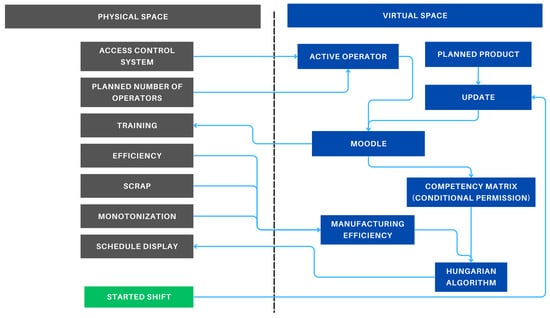
Figure 2.
New method.
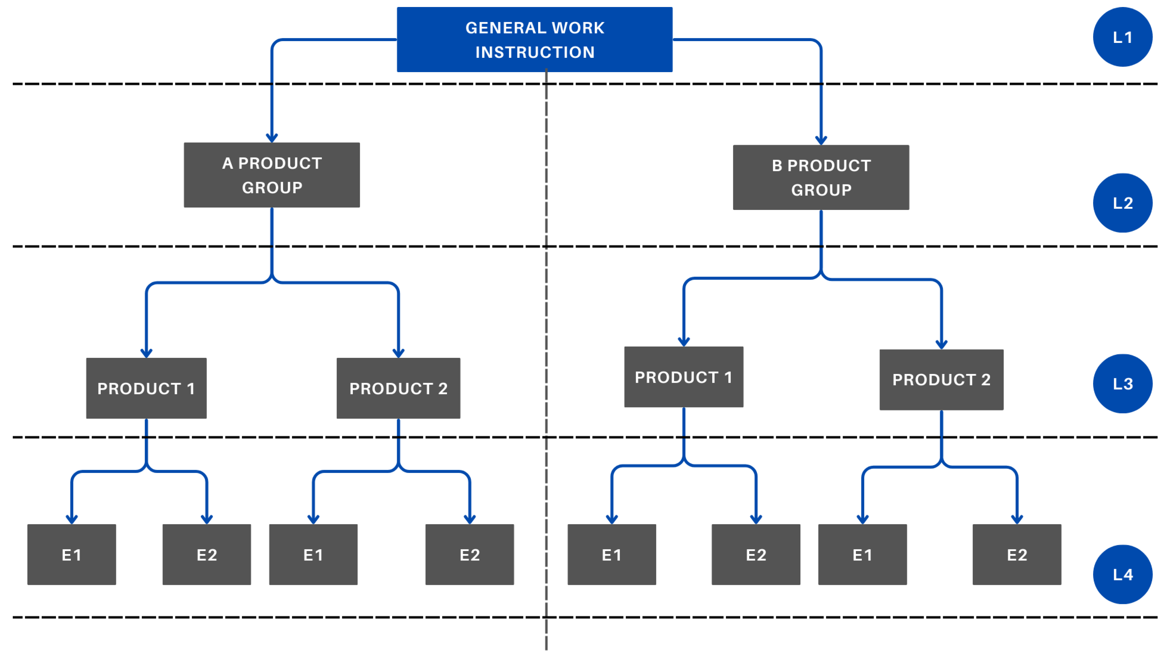
Based on the preliminary assessments, it became clear that there is a need for a new LMS that can support certain aspects of the new methods. Product training, health restrictions, and the complexity of product assembly are managed within a hierarchical model in the new Moodle system (Figure 3). Each product or product group is registered as a course, which is created and maintained by the administrators. Moodle provides an efficient platform for keeping operator qualifications up to date. Its use enables the visualization of the operators’ competency matrix, allowing for transparent and quick filtering.

Figure 3.
Hierarchical education model.
The general work instructions (fire safety, occupational safety, break schedule) are placed at the highest level of the hierarchy (L1). These are the training materials that the operator receives in all cases, and they are mandatory for performing the work. At the next level (L2), the work instructions for each product group (products belonging to the same product family) are located. These include the specific details related to the given product family (e.g., visual aids). The L3 level contains the training materials directly related to the specific product (e.g., packaging instructions). At the lowest level (L4), the extraordinary training materials are located. For an operator to manufacture a product, they must receive the relevant training for every level (L1–L4).
If an operator has a health issue (e.g., cannot perform standing work, cannot lift more than 5 kg), this information will be recorded in their profile upon entering the Moodle system. As a result, the operator will no longer be assigned to courses related to products they are not allowed to manufacture.
The products are divided into two groups based on their level of complexity. The shift leader determines, based on the operator’s prior performance, whether the operator is qualified to work with products that involve a more complex manufacturing process. Health and complexity restrictions are represented in a common matrix. Health and qualification regulations are strict constraints. There is no such thing as partial compliance, which is why we use binary notation. According to industrial standards, if someone is not in adequate health or lacks the required training, they are not allowed to perform any work. The purpose of this matrix is to clearly indicate when an operator is not permitted to carry out the task at a given moment.
For example, Product 1 is assigned to the number “12,” indicating that it has health restrictions, but its manufacturing process is not complex. In contrast, Product 2, represented by “03,” signifies a complex part without health restrictions. Operators can access the relevant training materials and complete the required tests by logging into their user accounts. For specific part training where instructor involvement is mandatory (e.g., for difficult-to-assemble categories), the instructor personally provides the necessary information. Afterward, the operator either completes a test independently or, if a test is not required, acknowledges and accepts the training information by reviewing the course.
The competency matrix is used to represent the knowledge of all available operators related to a specific product. If the value is 0, it means the operator has not received training for the product or cannot participate in its manufacturing (e.g., due to health restrictions); if the value is 1, it means the operator can manufacture the product and has valid training for the product. This restrictive matrix can be automatically generated based on the Moodle system.
Another important operator metric is the operator’s manufacturing efficiency. The company already measures the related data through another system. Manufacturing efficiency is a percentage value that indicates how quickly the operator produces the product according to the standard. This dataset has been defined as an efficiency matrix. If the operator has not yet manufactured the given product, or if there are no manufacturing data available due to the introduction of a new product, the default manufacturing efficiency value is set to 70% during the database query.
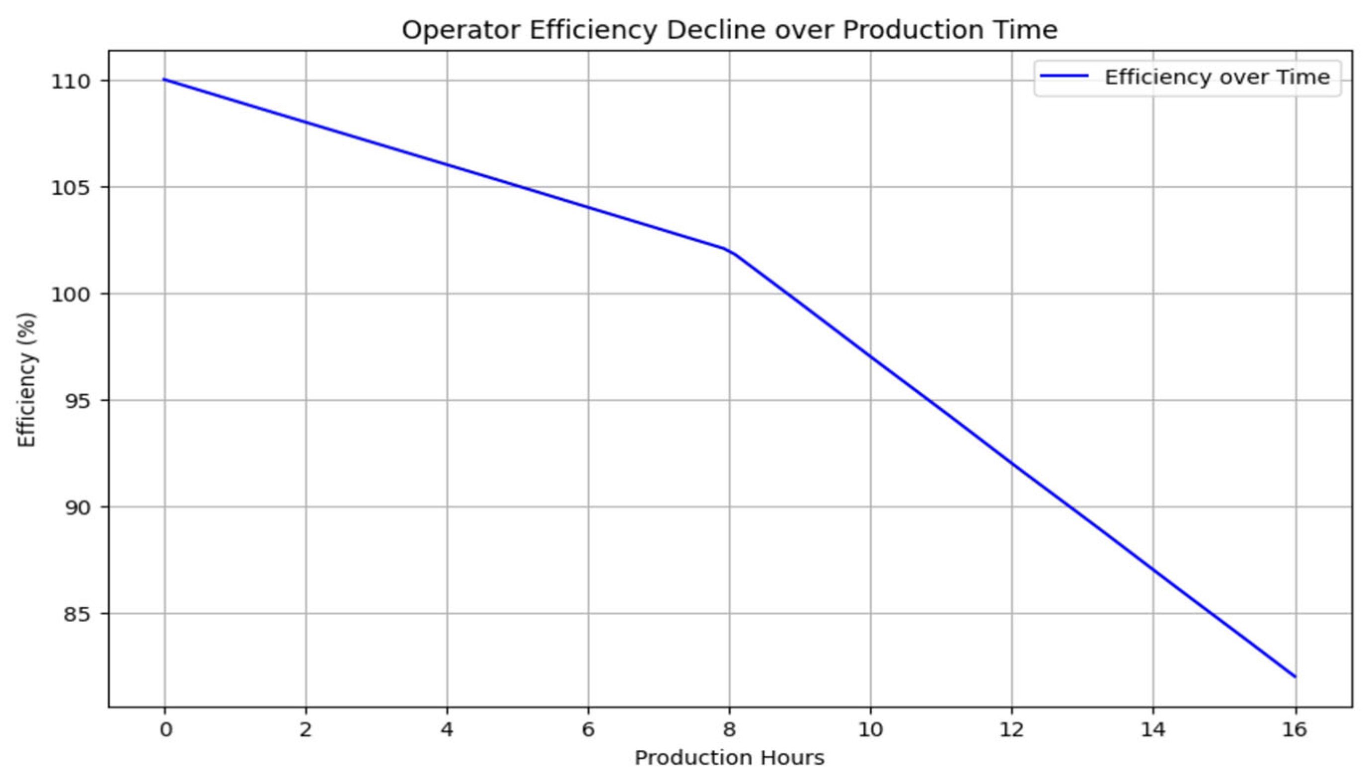
To mitigate monotony, the algorithm must account for whether an operator has manufactured the same product for two consecutive 8-h shifts in recent days. After 16 h of working on the same product, it is not advisable for the operator to continue manufacturing it. Additionally, it is important to prevent a scenario where an operator becomes proficient in only a limited range of products, resulting in low efficiency for others because the algorithm never assigns them to those tasks. This issue is addressed through a monotonicity function. During the first 8 h, efficiency decreases by 1% per hour, and after 8 h, it decreases by 2.5% per hour. For instance, with an initial efficiency of 110%, the manufacturing efficiency would drop to 82% after 16 h of production due to the monotonicity effect (Figure 4). This function can be further refined based on future data collection.
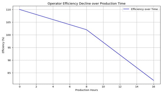
Figure 4.
Application of the monotonicity function.
The purpose of the function is to enforce the company’s prescribed regulations. In this case, the rule is a “soft” constraint. It is not recommended for an operator to produce the same product for more than 2 × 8 h. However, if available resources do not allow for sufficient variation, the regulation can be relaxed to meet production demands. The parameters of the monotony penalty were chosen based on ergonomic research demonstrating the effects of fatigue. The 1% per hour decrease during the first 8 h is a conservative estimate, while the 2.5% per hour decrease after 8 h aims to model the more pronounced impact, as supported by Folkard and others [18,19].
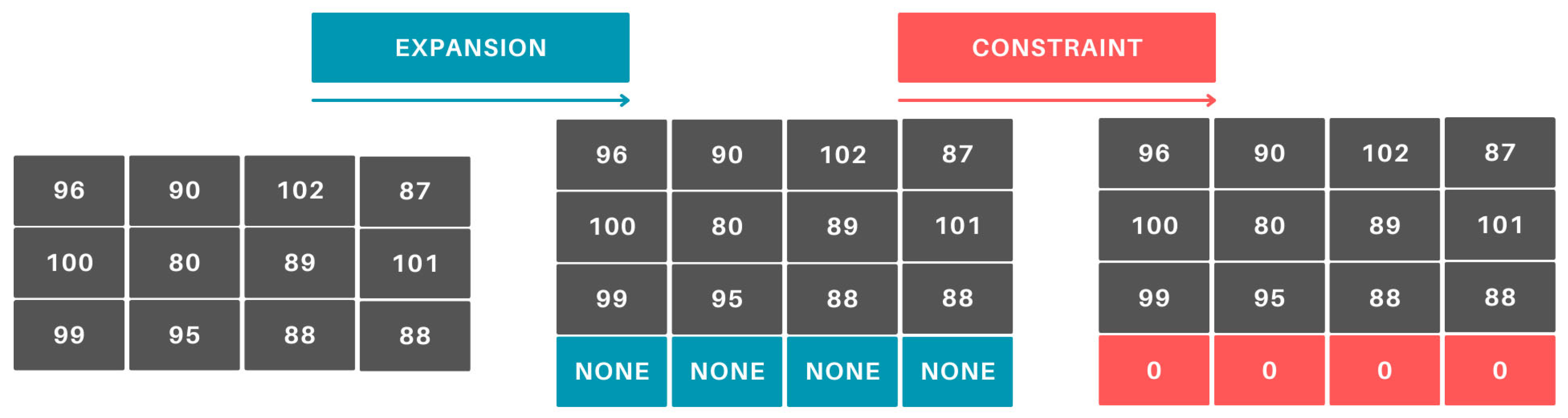
The Hungarian algorithm’s input matrix is constructed using the constraint matrix and the efficiency matrix. Since the algorithm can only optimize a square matrix, any non-square dataset must be supplemented with additional data to meet this requirement. If necessary, a row or column (as illustrated in Figure 5) is added to the efficiency matrix. In the constraint matrix, the corresponding values for the added row or column are set to 0, ensuring they are excluded from the optimization process.
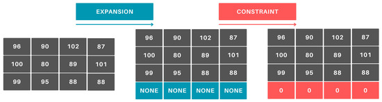
Figure 5.
Adding an extra row.
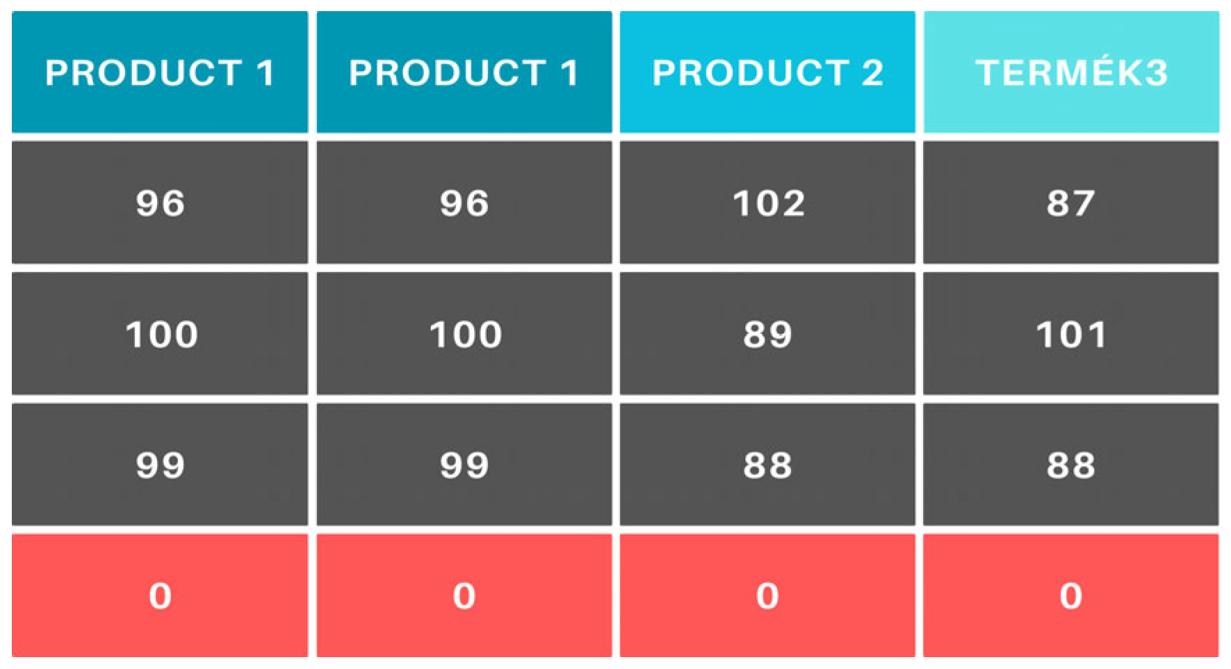
There are products where more than one operator is required for manufacturing. In this case, the product appears in the efficiency matrix column as many times as the number of operators required for its production (Figure 6).
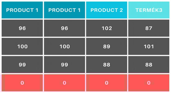
Figure 6.
Handling multi-operator products.
To determine the optimal task allocation, efficiency maximization must be converted into a minimization problem suitable for the Hungarian algorithm. This requires transforming the efficiency matrix into a cost matrix. The transformation is achieved by subtracting each value in the efficiency matrix from its maximum value, as described by Equation (1).
Equation (1). Creating a cost matrix.
- where
- Cij is the efficiency in the cost matrix at the i-th row and j-th column.
- Hmax is the largest value in the efficiency matrix.
- Hij is the efficiency value in the i-th row and j-th column of the cost matrix.
There is a linear relationship between the efficiency values. Based on predefined standards, efficiency values are determined as a function of time. Therefore, the equation provides sufficient information to represent the costs.
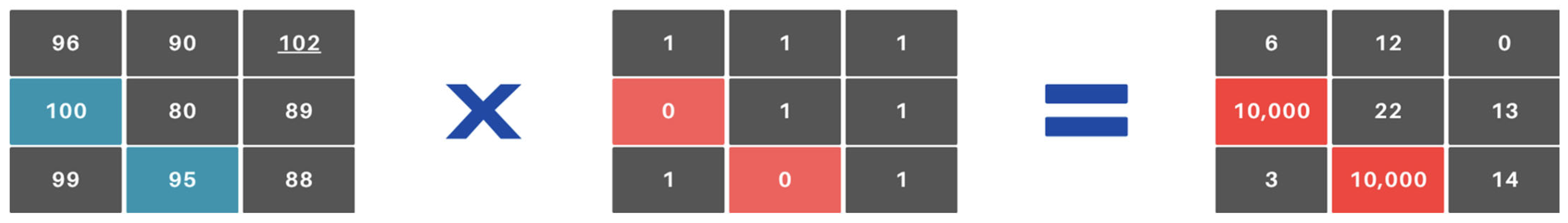
The constraint matrix must be applied to the resulting cost matrix. For the products that the operator cannot manufacture and, therefore, have a value of 0 in the constraint matrix, a high-cost value (10,000) is set (Figure 7).
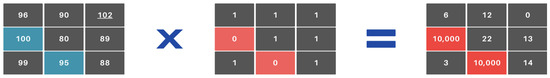
Figure 7.
Applying the constraint matrix.
In cases where an operator is excluded from producing a certain product due to a restriction, an exceptionally high constant cost is assigned. This ensures that, during optimization, the algorithm ranks the operator last for that product, increasing the likelihood of assigning them to a different product instead.
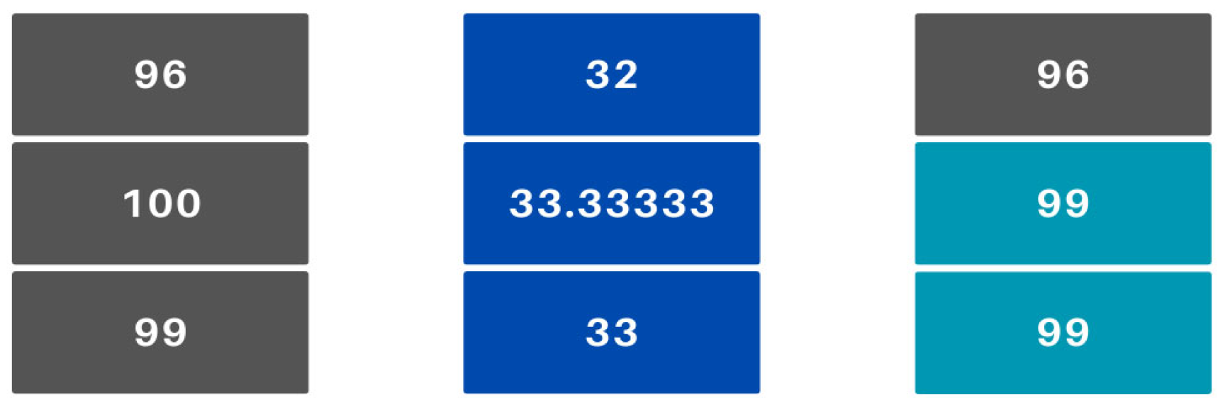
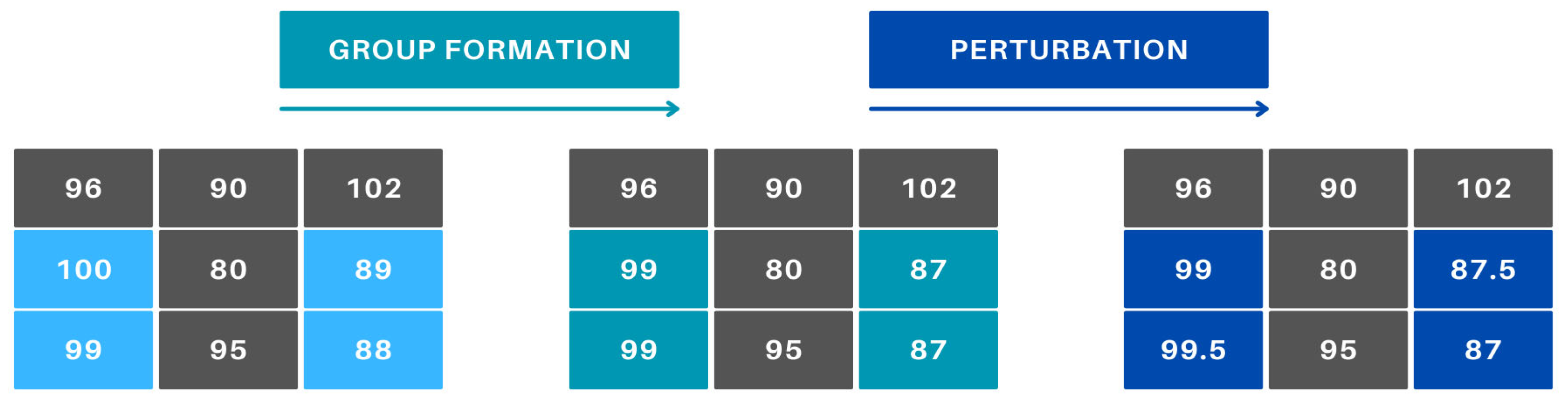
To prevent minimal differences in operators’ efficiency from disproportionately influencing the allocation results, similar efficiency values are grouped. This adjustment addresses the issue where a slightly better-performing operator would consistently be assigned the same task, potentially leading to monotony and limiting their experience with different products. The grouping process involves dividing each efficiency value by 3, retaining only the integer part of the result, and then multiplying this value by 3 (Figure 8). This ensures that efficiency within a ±1% range is treated as equivalent, promoting a fairer task distribution among operators.

Figure 8.
Grouping of similar efficiency values.
Within these groups, a perturbation ranging from −0.5 to 0.5 is applied to the efficiency values (Figure 9). This value has mathematical significance. By default, the algorithm always “rewards” the operator with higher efficiency, meaning lower cost. Therefore, we manipulate it randomly but deliberately, so that low-efficiency values do not distort the model. Preliminary experiments revealed that, when efficiency values are identical, the algorithm consistently selects the first operator in the order. This behavior would lead to the same monotonicity issue as when minimal efficiency differences exist. By adding a small random number, the monotonicity is disrupted while keeping the manufacturing efficiency effectively unchanged. This modification results in a suboptimal state. Nevertheless, we accept it because we are also considering other objectives and intentionally, under supervision, aim to manipulate the outcome to avoid monotony.
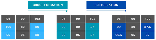
Figure 9.
Handling identical efficiencies.
The formal mathematical definition can be expressed for an n × n matrix [Equation (2)]. The term c₍ᵢⱼ₎ represents the cost of assigning operator i to task j. The variable x₍ᵢⱼ₎ is the decision variable, which takes the value 1 if operator i is assigned to task j, and 0 otherwise. These are binary variables, meaning their values are either 0 or 1. The objective is to assign each operator to at most one task, and ensure that each task is assigned to at least one operator [16].
Equation (2). Formalized mathematical definition.
The modifier rules used for the cost values generated for minimization are presented in Table 1.

Table 1.
Rules for generating production costs.
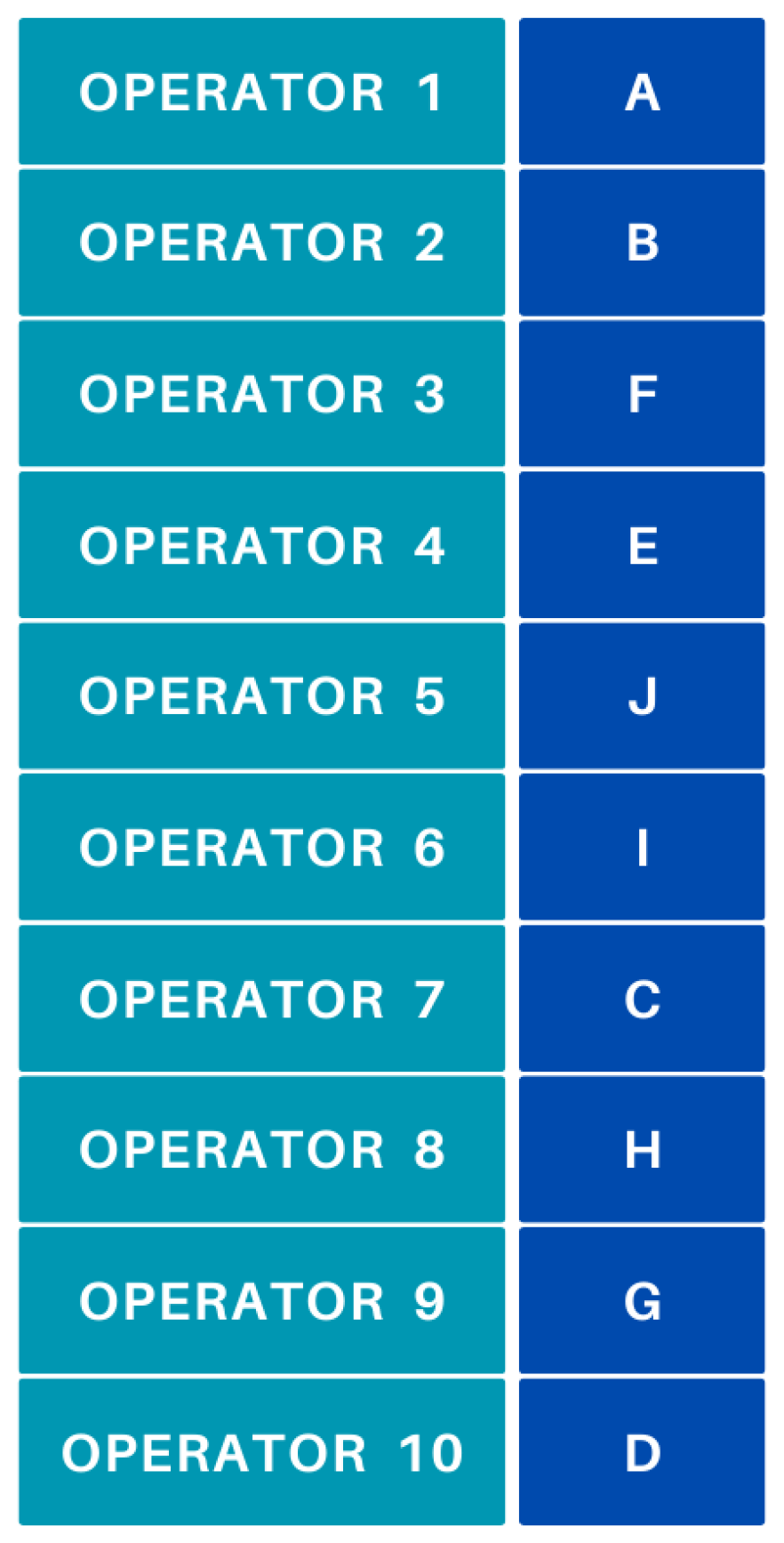
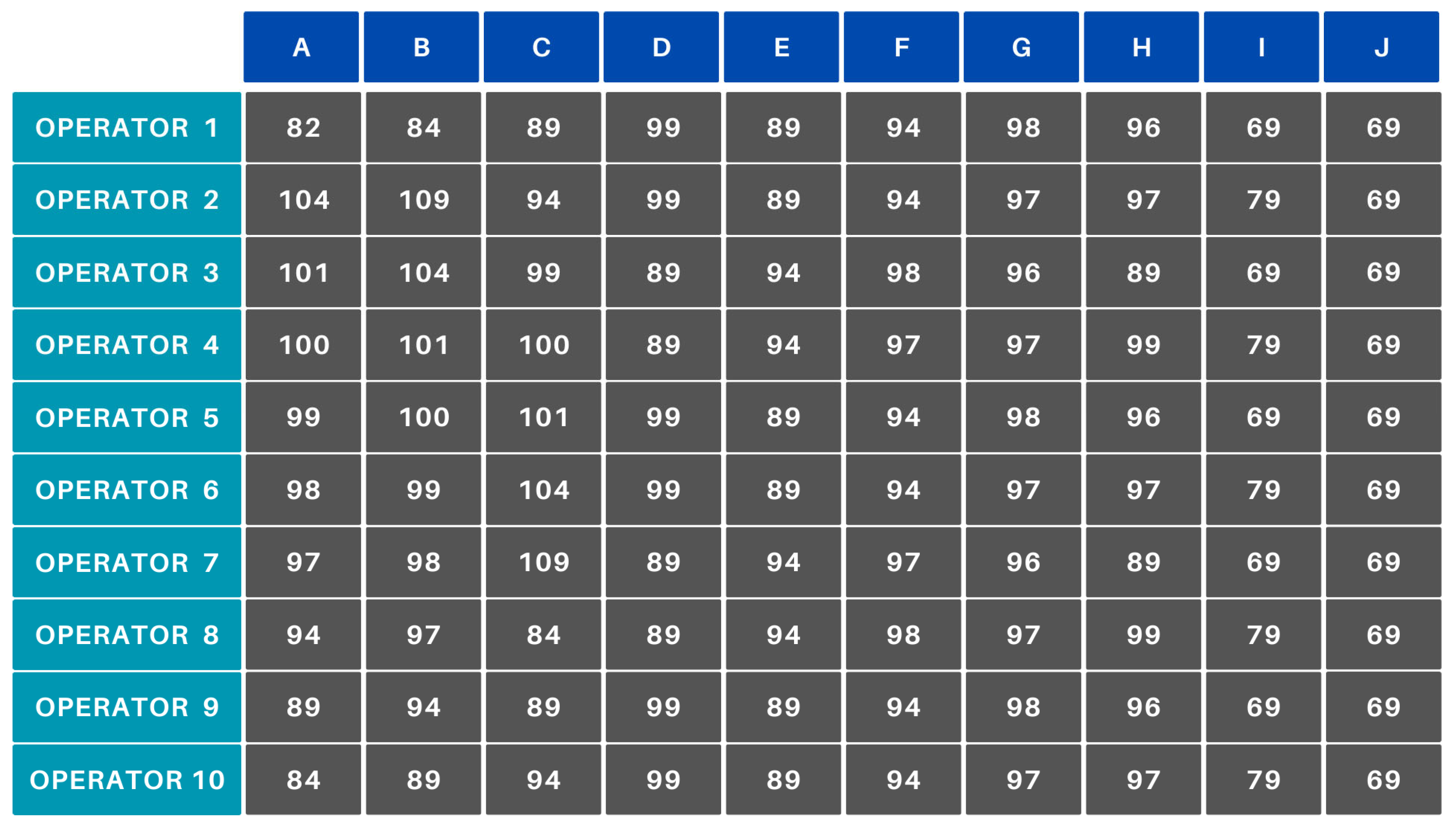
To validate the functionality of the newly created algorithm, several scenarios were examined. What they have in common is that an efficiency matrix was created for them (Figure 10), which can illustrate several industrial cases. Accordingly, the scenarios also validate extreme cases, such as when, for example, everyone produces product J with 70% efficiency. The tables below illustrate the results of the examined cases (A–F). Each table presents the assignments of 10 operators (Operator 1–Operator 10) to 10 products (A–J).

Figure 10.
Initial manufacturing efficiencies.
The data corresponding to points A–E were manually generated to ensure the reproducibility of the designated case. For point F, we used real company data extracted from the access and attendance tracking system employed by the company. These data are stored in an MSSQL database. The efficiency data were derived from the database of a data recording application developed by the company, operated by the machine operators, and supervised by the shift managers. The simulations were generated using a program written in Python 3.10.
The main parameters of the tasks performed were as follows:
- A total of 10 products, 10 operators, without monotony and restrictions.
- A total of eight products, 10 operators, without monotony and restrictions.
- A total of 10 products, eight operators, without monotony and restrictions.
- A total of 10 products, 10 operators, with monotony, without restrictions.
- A total of 10 products, 10 operators, with monotony, with restrictions.
- Real company data. Applicable and integrable from a conceptual perspective.
If a new product is added to the portfolio or a new operator joins the team and there are no manufacturing data available for efficiency, it is set to 70%. In the simulations, column J represents a new product. A cost matrix was generated from the base efficiency matrix. The result corresponding to scenario A is shown in Figure 11.
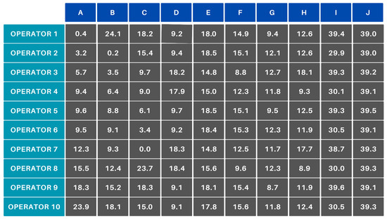
Figure 11.
Scenario A—cost matrix.
The table shows that, although the product in column J has not been manufactured yet, it has very similar costs to the product in column I, which has been manufactured previously. This avoids the problem of optimization where manufacturing a new product would result in an extreme cost function. At the same time, it is also important to consider that starting with a completely new product at the beginning of a shift is not advisable; so, a lower initial efficiency value typically meets both expectations. The latter is true when, at the beginning of the shift, more products are waiting production than the number of operators starting work. From an industrial perspective, this would be a contradiction. Running the Hungarian algorithm on the square cost matrix yields the result shown in Figure 12.
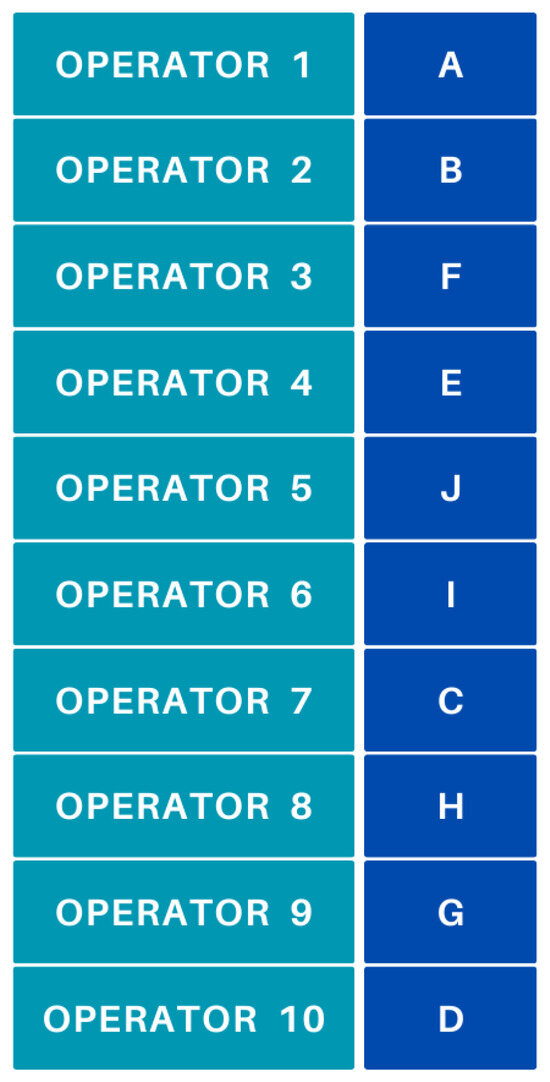
Figure 12.
Scenario A—optimal task allocation.
For additional validation of the method, the algorithm was run in a case where every operator manufactured every product with 100% efficiency. However, the matrix was created such that the manufacturing efficiency on the diagonal was set to 105%. In this case, the expected result was obtained, where the system allocated the products to the operators in the optimal order (A–J), as anticipated.
In scenario B, Operators 6 and 10 did not receive any parts, as there were only eight products to be allocated among 10 operators. The algorithm added two technical columns (I’ and J’) to the cost matrix (Figure 13) with an initial efficiency value of 0. After applying Equation (1), these technical products took on costs around 110–111, which caused them to be deprioritized during the optimization process. Although the algorithm logically assigned the I’ and J’ products to Operators 6 and 10, the actual delegation did not occur because the products do not physically exist.
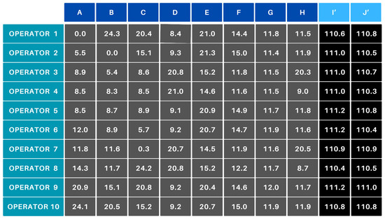
Figure 13.
Scenario B—cost matrix.
In scenario C, like the previous test, imaginary rows (operators) are assigned. However, in this case, the cost matrix is expanded with two ‘extra’ operators, assigned the highest cost values (Figure 14).
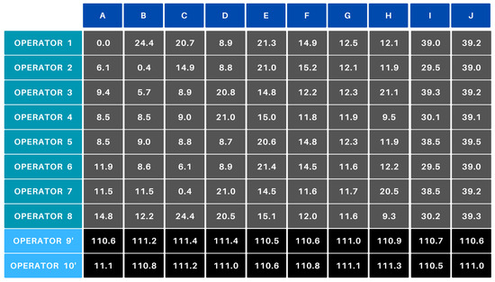
Figure 14.
Scenario C—cost matrix.
In daily operations, this scenario is typical, where the production plan usually requires manufacturing more parts than there are workers available. In such cases, when two operators are absent, two new rows need to be created in the cost matrix, and the 0-efficiency values are assigned a cost of around 110. During the allocation, these two extra operators will also be assigned work, but the associated products will remain queued for production. When a new operator arrives or a previous product is completed, the respective operator will take over the next product in line.
In scenario D, monotonicity was also considered. In this case, a high value was applied only to Operator 1 for Product A (who has been manufacturing this product for 16 h). As a result, their efficiency visibly dropped from 110% to 82% (Figure 10 vs. Figure 15). For the other operators, the hourly 1% decrease in efficiency is observed due to the 1-h manufacturing time.

Figure 15.
Scenario D—result with monotonicity.
After applying the subsequent steps (perturbation, cost matrix creation, constraints), the cost matrix used for optimization (minimization) was obtained. The application of monotonicity resulted in Operator 1 not manufacturing Product A, but instead Product J, which naturally impacted the allocation of other operators to products as well.
In scenario E, the efficiency matrix was modified. For Operator 1, the efficiency for Product E was set at 120%. By running the algorithm 10 times, it was verified that Operator 1 consistently received Product E. Afterward, Product E was excluded from the constraint matrix, causing Operator 1 to no longer be assigned to Product E. In the cost matrix, compared to the default case (Figure 11), the costs significantly increased, with an approximate rise of 10,000.
The integrability of the new algorithm into a real corporate environment was examined. The algorithm retrieves the attendance records of operators from the Seawing access control system, which includes the arrival times of operators present at the company. The efficiency data are determined based on information from the operator production-following system, which was previously developed and used within the company. The matrix of operator qualifications is available from the LMS Moodle system, providing the necessary data for defining the constraint matrix. Accurately determining the manufacturing efficiency of operators is crucial. Currently, the company uses a norm-based efficiency calculation, which compares the quantity produced by the operator and the corresponding production time to the prescribed norm. However, this method can be inaccurate in some cases. For example, if Operator 1 produces 1 box (a small quantity) with 100% efficiency, and Operator 2 produces 20 boxes (a larger quantity) with 80% efficiency, Operator 1 may appear to have better efficiency, even though Operator 2 is handling a significantly larger volume. However, this is not always certain, as Operator 1 may produce the next product at only 75% efficiency, possibly for an extended period. Additionally, if an operator completes one box at 100% efficiency at the beginning of the shift but does not work for the remainder of the shift, it will appear as if they performed at 100% efficiency, even though their output for the rest of the shift is zero. Accurately determining efficiency is a complex task, and while this research does not address the methodology for this, it is important to highlight the potential problems. It is assumed that, within the norm-based efficiency system, each operator performs their work according to the prescribed standards. During testing, it became clear that the default efficiency for newly added products and operators cannot be set to 0%, as this results in values like those created by fictitious rows or columns. The 70% value is subject to modification based on further data collection. Another important parameter in the algorithm is the monotonicity function. The 16-h time frame was objectively determined based on the experience of production managers, though the foundations of this determination were not examined in this research. From an optimization perspective, it is evident that the monotonicity effect resulting from monotonous work on the production line, whether positive or negative, must be addressed. Simulations based on company data have demonstrated that the algorithm and coding method are also suitable for integration in industrial environments. The Python programming language, which is well-known in the industry, provides an efficient development environment. It integrates seamlessly with most databases, is user-friendly, and is highly adaptable for future development.
We examined the algorithm in terms of time efficiency. Shift supervisors spend approximately 6–8 min starting a shift. In the tested cases with 20–25 personnel and running the algorithm 30 times, the longest runtime was 73 s. This duration also includes the time the program spends gathering data (retrieving efficiency data from the database, downloading attendance records, and loading the list of products to be manufactured). The time efficiency, calculated using Equation (3), is approximately between 79.72% and 82.79%.
Equation (3). Time efficiency.
In practice, it can be significantly more efficient than this. Ideally, shift supervisors do not need to intervene at all, as employees can read from a monitor placed for operators which workstation they should start working at, eliminating the need for any interaction with the shift supervisor.
The method can be generalized to other industries where tasks are assigned to one or more executors. It is important that these assignments can be represented with a cost value. A suitable competency matrix must be created to characterize the task executors. Table 2 contains a general description of the components of the method.
Table 2.
General description of the components of the method.
5. Conclusions
Automation and optimization of processes are ongoing priorities for manufacturing companies, as they significantly impact production efficiency, cost-effectiveness, and competitiveness. For automation to succeed, it is essential to thoroughly analyze the processes and identify issues in a comprehensive manner. The success of automation largely depends on how accurately the development team identifies the root causes of the problems and how effectively they choose the methods and tools to address them. As a result of a comprehensive internal survey, a method was developed that incorporates the company’s needs, making them processable by the algorithm. The core optimization method can be seen as a foundation, around which real-world solutions are organized. This complex process, illustrated in Figure 2, is achieved through additional matrices and extreme low or high exclusion values.
The scenarios conducted demonstrated that, after modifying the input conditions and parameters, optimization with the Hungarian algorithm works effectively. A key factor was ensuring that the cost matrix used for optimization was logically structured from a workforce planning perspective, considering both industry standards and the company’s internal regulations. The tests also revealed that, according to the algorithm’s principles, products that can be manufactured with high efficiency should be prioritized for assignment. This approach greatly aids employees in starting the shift with minimal issues. As workers settle into their tasks and assemble the first product in the series, they can progress to the more challenging products. Since this progression does not occur simultaneously, the production manager overseeing the shift can focus more on these transitions and intervene if necessary. During the training sessions, we verify understanding and provide the opportunity to ask for help. On the other hand, the employees’ work is continuously monitored by shift supervisors (who track performance), and assistance can also be requested during work if needed. Based on feedback from the shift supervisors, the operators began their shifts more efficiently.
It can be concluded that the newly developed method addresses the requirements and helps reduce administrative tasks. A notable opportunity that arises from the start of shift is that operators who arrive earlier receive the easier-to-manufacture products first, which could even encourage operators to arrive at their workplace on time.
6. Future Work
The algorithm does not handle shift changes and transitions during shifts. The system can be further developed, but the reasons and processes of these transitions must be precisely assessed. Additional development is needed to optimally determine the products to be manufactured. Currently, the system allocates data based on a non-optimized production plan. Due to improperly selected products, the area’s efficiency will not achieve the expected improvement. After collecting data for 6–12 months, we need to analyze how often shifts actually started according to the generated schedules and how much the time between the start of manufacturing the first box and the theoretical shift start has decreased.
Author Contributions
Conceptualization, G.L. and M.A.; methodology, G.L.; software, G.L.; validation, M.A. and B.Z.V.; formal analysis, I.A.; investigation I.A. and B.Z.V.; resources, I.A. and B.Z.V.; data curation, G.L.; writing—original draft preparation, G.L. and M.A.; writing—review and editing, G.L. and M.A.; visualization, G.L.; supervision, M.A.; project administration, G.L. All authors have read and agreed to the published version of the manuscript.
Funding
This research received no external funding.
Data Availability Statement
https://github.com/lakatosgabor/magyar_modszer/blob/main/operator_booking_data.csv (accessed on 26 July 2025).
Conflicts of Interest
The authors declare no conflict of interest.
References
- Ghoushchi, S.J.; Abbasi, A. An optimisation approach for simulation operator allocation and job dispatching rule in a cellular manufacturing system. Int. J. Serv. Oper. Manag. 2021, 40, 47–67. [Google Scholar] [CrossRef]
- Song, B.L.; Wong, W.K.; Fan, J.T.; Chan, S.F. A recursive operator allocation approach for assembly line-balancing optimization problem with the consideration of operator efficiency. Comput. Ind. Eng. 2006, 51, 585–608. [Google Scholar] [CrossRef]
- Gawas, P.; Legrain, A.; Rousseau, L.M. Personnel Scheduling with flexibility for On-Call Shifts. arXiv 2023, arXiv:2312.06139. [Google Scholar] [CrossRef]
- Liu, T.; Zhang, L. Apply artificial neural network to solving manpower scheduling problem. In Proceedings of the 2021 IEEE 4th International Conference on Big Data and Artificial Intelligence (BDAI), Qingdao, China, 2–4 July 2021; pp. 58–64. [Google Scholar]
- Li, D.C.; Lin, Y.S. Learning management knowledge for manufacturing systems in the early stages using time series data. Eur. J. Oper. Res. 2008, 184, 169–184. [Google Scholar] [CrossRef]
- Davis, B.; Carmean, C.; Wagner, E.D. The Evolution of the LMS: From Management to Learning; e-Learning Guild: Santa Rosa, CA, USA, 2009. [Google Scholar]
- Patel, D.; Patel, H.I. Blended learning in higher education using MOODLE open source learning management tool. Int. J. Adv. Res. Comput. Sci. 2017, 8, 439–441. [Google Scholar]
- Chavan, A.; Pavri, S. Open-source learning management with Moodle. Linux J. 2004, 128, 2. [Google Scholar]
- Cole, J.; Foster, H. Using Moodle: Teaching with the Popular Open Source Course Management System; O’Reilly Media: Sebastopol, CA, USA, 2007. [Google Scholar]
- Rusdiana, S.; Oktavia, R.; Charlie, E. Application of Hungarian method in optimizing the scheduling of employee assignment and profit of home industry production. J. Res. Math. Trends Technol. 2019, 1, 24–33. [Google Scholar] [CrossRef]
- Kuhn, H.W. The Hungarian method for the assignment problem. Nav. Res. Logist. Q. 1955, 2, 83–97. [Google Scholar] [CrossRef]
- Koliński, A.; Koliński, M. The use of Hungarian method in the evaluation of production efficiency. In Innovations in Management and Production Engineering; Publishing House of Polish Association for Production Management: Opole, Poland, 2013; pp. 116–127. [Google Scholar]
- Bai, X.; Yan, W.; Ge, S.S.; Cao, M. An integrated multi-population genetic algorithm for multi-vehicle task assignment in a drift field. Inf. Sci. 2018, 453, 227–238. [Google Scholar] [CrossRef]
- Bai, X.; Yan, W.; Cao, M.; Xue, D. Distributed multi-vehicle task assignment in a time-invariant drift field with obstacles. IET Control Theory Appl. 2019, 13, 2886–2893. [Google Scholar] [CrossRef]
- Shrestha, D.; Wenan, T.; Shrestha, D.; Rajkarnikar, N.; Jeong, S.-R. Personalized Tourist Recommender System: A Data-Driven and Machine-Learning Approach. Computation 2024, 12, 59. [Google Scholar] [CrossRef]
- Pires, E.J.S.; Cerveira, A.; Baptista, J. Wind Farm Cable Connection Layout Optimization Using a Genetic Algorithm and Integer Linear Programming. Computation 2023, 11, 241. [Google Scholar] [CrossRef]
- Solve the Linear Sum Assignment Problem with Python Function. Available online: https://docs.scipy.org/doc/scipy/reference/generated/scipy.optimize.linear_sum_assignment.html (accessed on 19 November 2024).
- Folkard, S.; Lomb, D.A. Modeling the impact of the components of long work hours on injuries and “accidents”. Am. J. Ind. Med. 2006, 49, 953–963. [Google Scholar] [CrossRef] [PubMed]
- Åkerstedt, T. Work hours, sleepiness and the underlying mechanisms. J. Sleep Res. 1995, 4, 15–22. [Google Scholar] [CrossRef] [PubMed]
- Ivanova, V.S.; Mertins, K.V.; Abdrashitova, M.O.; Isaeva, D. Active learning approach in Moodle for the organization of student’s self-study practice-based learning activities. In Proceedings of the MATEC Web of Conferences, Tomsk, Russia, 12–14 April 2016; Volume 48, p. 6005. [Google Scholar]
- Santoso, I.; Efendy, I. Usability study of moodle LMS in statistics Indonesia learning center-case study. J. Phys. Conf. Ser. 2020, 1511, 012023. [Google Scholar] [CrossRef]
- Jackson, E.A. MOODLE Platform: A case of flexible corporate learning in the financial sector in Sierra leone. In Trends in E-Learning; Intechopen: London, UK, 2018. [Google Scholar]


Disclaimer/Publisher’s Note: The statements, opinions and data contained in all publications are solely those of the individual author(s) and contributor(s) and not of MDPI and/or the editor(s). MDPI and/or the editor(s) disclaim responsibility for any injury to people or property resulting from any ideas, methods, instructions or products referred to in the content. |
© 2025 by the authors. Licensee MDPI, Basel, Switzerland. This article is an open access article distributed under the terms and conditions of the Creative Commons Attribution (CC BY) license (https://creativecommons.org/licenses/by/4.0/).