Abstract
Kidney-paired donation programs assist patients in need of a kidney to swap their incompatible donor with another incompatible patient–donor pair for a suitable kidney in return. The kidney exchange problem (KEP) is a mathematical optimization problem that consists of finding the maximum set of matches in a directed graph representing the pool of incompatible pairs. Depending on the specific framework, these matches can come in the form of (bounded) directed cycles or directed paths. This gives rise to a family of KEP models that have been studied over the past few years. Several of these models require an exponential number of constraints to eliminate cycles and chains that exceed a given length. In this paper, we present enhancements to a subset of existing models that exploit the connectivity properties of the underlying graphs, thereby rendering more compact and tractable models in both cycle-only and cycle-and-chain versions. In addition, an efficient algorithm is developed for detecting violated constraints and solving the problem. To assess the value of our enhanced models and algorithm, an extensive computational study was carried out comparing with existing formulations. The results demonstrated the effectiveness of the proposed approach. For example, among the main findings for edge-based cycle-only models, the proposed (*PRE(i)) model uses a new set of constraints and a small subset of the full set of length-k paths that are included in the edge formulation. The proposed model was observed to achieve a more than 98% reduction in the number of such paths among all tested instances. With respect to cycle-and-chain formulations, the proposed (*ReSPLIT) model outperformed Anderson’s arc-based (AA) formulation and the path constrained-TSP formulation on all instances that we tested. In particular, when tested on a difficult sets of instances from the literature, the proposed (*ReSPLIT) model provided the best results compared to the AA and PC-based models.
1. Introduction
The kidney exchange problem (KEP) is a combinatorial optimization problem that aims to maximize the number of patient–donor matches as represented by cycles or paths in a directed graph. The KEP has received increased attention over the past few years, with several different versions implemented worldwide through different kidney paired donation programs. The need for such a program in the U.S., for example, was outlined by Ross et al. [1], who cited four motivating factors: (a) high demand for kidneys among the population, (b) relatively low number of cadaveric (deceased) donors compared to the demand, (c) growing wait lists, and (d) the very high cost of kidney-related treatments such as hemodialysis. Several researchers have addressed each of these factors from a clinical perspective [2]. Others have taken a prescriptive approach and developed optimization models to aid decision-makers. The first such models were presented by [3,4,5]. Subsequently, there has been a spate of research ranging from model development, to ways of handling different versions of the problem, to dealing with uncertainty in donor–patient matches.
Depending on the specific application, matches can come in the form of directed cycles or directed paths. A cyclic exchange is when a living donor who is incompatible with the intended recipient (this is called an incompatible patient–donor pair (PDP)) offers a kidney to another patient conditioned on the donor’s intended recipient receiving a compatible kidney from another person (see Figure 1). Such exchanges are known as k-way cyclic exchanges, where k is the number of incompatible PDPs involved in the cycle. In a cyclic exchange, the patient in the first PDP risks not receiving a kidney in return if subsequent exchanges in other PDPs fail to proceed to transplantation. To eliminate such risk, surgeries in cyclic exchanges are conducted simultaneously. This requirement greatly increases the need for available operating rooms and surgical teams at specified times and dates ( in each case for every k-way cyclic exchange). For example, a three-way cycle involves the simultaneous coordination of six operating rooms and six surgical teams. Given this burden, cyclic exchanges with more than three patient–donor pairs are rarely conducted [6].
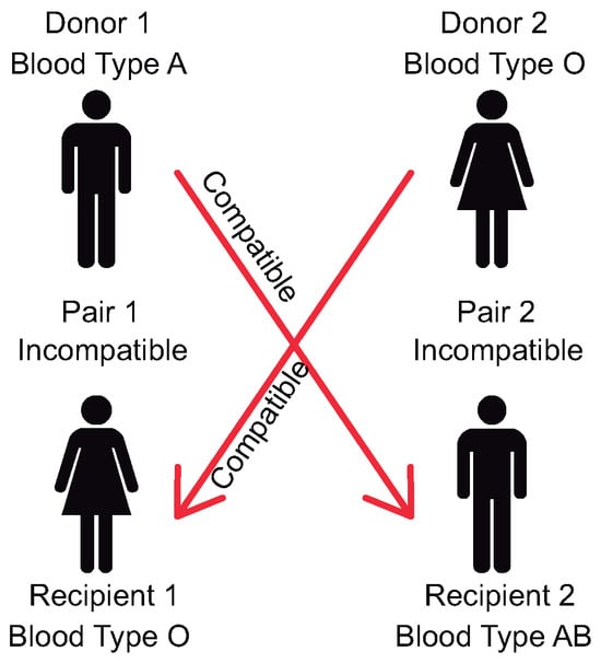
Figure 1.
Two-way cycle.
A path (or chain) exchange arises when a non-directed donor (NDD) (i.e., an altruistic person who decides to donate without having an intended recipient) offers a kidney to a patient associated with a particular PDP. The donor in this pair is then matched with a patient of another PDP, and so forth, forming a chain with the NDD and L recipients (see Figure 2) in which the donor in the last PDP in the chain either donates to a patient on a waiting list or is considered as an NDD in the next algorithm run. When a chain is initiated by an NDD, it can be structured to ensure that no donor in a pair has to donate a kidney before the corresponding patient has received one, allowing the simultaneity requirement to be relaxed.
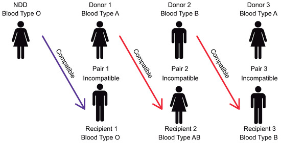
Figure 2.
Chain with length of 3.
The maximum size of chains and cycles is determined by each kidney paired donation program. An ongoing debate around chains is whether or not they should be performed simultaneously. Under the domino-paired donation scheme [7], an NDD triggers a short simultaneous chain, with the donor in the last pair donating to a candidate on the waiting list for a cadaveric organ. The other scheme is the non-simultaneous extended altruistic donor chain [8,9,10], under which the NDD initiates a theoretically never-ending chain consisting of several short segments, each of which is carried out simultaneously. The last donor in each segment becomes a bridge donor who can initiate the next chain segment at some later time unless they drop out. When the solution can be in the form of unbounded chains or cycles, the KEP turns into the problem of maximum weighted perfect matching on a bipartite graph [11], which can be solved in polynomial time. When only two-way cycle exchanges are allowed, the KEP is equivalent to the maximum matching problem, which is also solvable in polynomial time with Edmonds’ maximum cardinality matching algorithm [12]. The general problem with k-way cyclic exchanges is that they are known to be strongly NP-hard for [11,13].
Current work on solving the KEP is dominated by exact approaches based on integer programming (IP) formulations. Some IP models use a considerably large number of constraints or variables, often exponential in number. This limits the size of an instance that can be solved to optimality.
In this paper, we introduce three new models that extend several existing formulations. With the help of special network connectivity properties, we show that many of the current models can be significantly reduced in size without compromising their correctness. The improvements we have developed are based on detecting strong connectivity in the underlying graphs, especially for medium-sized instances. In particular, this is the case for the edge formulation proposed by Abraham et al. [11] and Roth et al. [14], which is impractical even for small instances [11,15,16] as it requires constraints for graphs with m (directed) edges.
One of the primary contributions of our work is the identification of a special graph structure that allows us to significantly reduce the number of constraints as well as the number of paths needed in the edge formulation of the KEP. In addition, we replace the cycle-cardinality constraints in the edge formulation by tournament inequalities, which have been shown to be valid and facet-defining for the cycle-only version [17,18]. A related contribution is our design and development of an efficient algorithm for applying the proposed reduction and building the corresponding models.
Testing was performed over a wide range of instances found in the literature. The performance of our cycle-only and cycle-and-chain versions of the KEP was compared with the performance of the most relevant previously-developed models. In terms of cycle-only models, the state of the art reveals both non-compact (exponentially-sized) formulations [11,14] and compact formulations [15]. In general terms, the former have been found to be more effective, particularly the cycle formulation. However, a study by Constantino et al. [15] showed that compact formulations have poor performance at solving instances larger than 50 pairs, where they are much less effective. For example, the non-compact cycle formulation was found to be very efficient for low-density graphs with small values of k; however, the non-compact formulation becomes inefficient for larger values of k, especially as the graphs become more dense. In such cases, compact formulations provide better results and are able to solve larger problems.
The results indicate that our formulations for the cycle-only setting are able to solve practical instances with low-density to medium-density graphs in remarkably less time than the classical edge formulation while finding many more optimal solutions within the imposed time limit. For the cycle-and-chain formulations, the results show that our approach is superior with respect to two out of the three existing formulations we tested, and is competitive with the formulation that provided the shortest running times and greatest number of optimal solutions. In sum, our main contribution lies in providing models and an accompanying solution methodology that considerably reduces the size of the problem (in terms of the number of constraints) with respect to KEP models based on an exponential number of constraints.
The remainder of this paper is organized as follows. In Section 3, the general version of the KEP is defined and some special cases are identified. This is followed by a literature review in Section 2. In Section 4, three new formulations are introduced that take advantage of certain network connectivity properties. The discussion includes a comparison of the linear programming relaxations of the corresponding models. In Section 5, we present the proposed solution algorithm, followed in Section 6 by the results of our computational experiments comparing the performance of the new and existing formulations. Section 7 concludes with a discussion of the our findings and several observations on the value of the research. Finally, we offer a number of avenues for future work.
2. Literature Review
The concept of kidney exchange was first presented by Rapaport [19]. Later, Ross et al. [1] and Ross and Woodle [20] discussed its ethical aspects. Roth et al. [3] first proposed organizing kidney exchanges on a large scale and applying operations research methods to solve the KEP (also see Roth et al. [4,21]).
2.1. Cycle-Only Formulations
Abraham et al. [11] and Roth et al. [14] introduced the first two IP models for the cycle-only case, which consisted of the cycle formulation and edge formulation. The former includes one binary decision variable for each feasible cycle, while the latter includes one binary decision variable for each arc in the graph for each compatible pair. In the cycle formulation, the number of constraints is polynomial in the size of the input, but the number of variables is exponential. In the edge formulation, the number of variables is polynomial, while the number of constraints is exponential. Abraham et al. [11] reported experimental results with simulated test instances (as proposed by Saidman et al. [22]) with up to 10,000 incompatible pairs for the cycle formulation by means of a branch-and-price algorithm for . It is worth noting that the graph density of the examined instances was not reported; to the best of our knowledge, state-of-the-art branch–cut–price algorithms have now reported results with up to 2048 pairs [18].
The initial models proposed for kidney exchange programs had exponential numbers of constraints or variables. Constantino et al. [15] presented the first two compact IP formulations for the cycle-only KEP that included the edge assignment formulation and the extended edge formulation. A compact formulation is polynomially bounded in both the number of variables and number of constraints. For testing purposes, they randomly generated instances with correspondingly low-, medium-, and high-density graphs, the largest of which had 1000 incompatible patient–donor pairs.
2.2. Cycle-and-Chain Formulations
Mak-Hau [16] introduced a compact formulation (denoted as EE-MTZ) that integrates chains and cycles. This formulation uses the extended edge formulation to address cycles, while a variant of the Miller–Tucker–Zemlin inequalities for the traveling salesman problem (TSP) is used to model chains. They also proposed an exponential version of the EE-MTZ formulation that handles cycles in the same way that the edge formulation does. The largest instance that they tackled consisted of 256 PDPs and six NDDs.
Anderson et al. [8] introduced two formulations for the KEP with bounded cycle lengths and unbounded chain lengths. The first consisted of an arc-based model that uses binary variables to represent the selection of arcs. This leads to an exponential number of constraints in order to prevent cycle lengths greater than k (cycle-cardinality constraints). The second, called the PC-TSP-based formulation, uses an exponential number of binary variables to represent cycles, but also requires an exponential number of constraints. For the first model, they presented a solution algorithm that relaxes the cycle-cardinality constraints (but not the integrality constraints), then iteratively adds them back as needed while solving an IP at each iteration. This approach can be called branch–bound–cut. For the second model, they implemented a branch-and-cut algorithm. Testing was performed using randomly generated instances based on data from the National Kidney Registry and the Alliance for Paired Donation pool. The largest instances they tried to solve contained up to 700 PDPs and 175 NDDs.
Inspired by the extended edge formulation and the cycle formulation, Dickerson et al. [23] presented three IP formulations using position-indexed variables,. Along with simulated data, they analyzed real instances obtained from the United Network for Organ Sharing (UNOS) in the U.S. and from the U.K. kidney exchange program (NLDKSS). On average, the UNOS instances contained 231 PDPs and two NDDs (UNOS runs the algorithm twice a week, keeping the number of altruists small), while the NLDKSS instances contained 201 PDPs and seven NDDs. The simulated data were based on historical UNOS data, with up to 700 PDPs and 175 NDDs.
2.3. Column and Constraint Generation Algorithms
To avoid the need to keep the entire model in memory, several different branch-and-price and branch-and-cut algorithms have been proposed. The fastest exact algorithms to date use column generation to find solutions to the cycle [11,18,23,24,25,26] and cycle-and-chain models Riascos-Álvarez et al. [27], Arslan et al. [28] of the KEP. The only two approaches that we are aware of that use constraint generation were presented by Anderson et al. [8] and Lam and Mak-Hau [18]. The former used an arc-based formulation to address chains and the cycle formulation for cycles. The solution was obtained with a branch-and-bound algorithm, which proved to be effective for solving instances with a cycle-length limit of 3 and unbounded chain lengths. However, the same algorithm proved uncompetitive when compared to branch-and-price-based approaches when the chain size is constrained [25]. To date, the latter of these, which tackles the cycle-only version, remains the only branch–cut–price algorithm. Results were provided for instances with up to 2048 pairs and .
2.4. Other KEP Studies
Alternatives to the objective of finding the maximum number of exchanges or maximum weighted sum of all exchanges include maximizing the expected number of transplants [24,29,30] and lexicographic optimization of a hierarchy of objectives [26,31]. Klimentova et al. [32] studied a stable KEP with preferences of patients over potential donors, where the objective is to find stable exchanges with the maximum cardinality. Other variations of the KEP have considered multiple donors associated with a single patient, where at most one patient is permitted to be in the final solution [11]. Another version allows compatible pairs to participate in kidney paired donation programs as long as the patient in that pair receives a “better” match than his current donor [33]. The purpose of this requirement is to increase the potential number of matches in a final solution that otherwise could not be reached without the inclusion of compatible pairs. Dickerson et al. [34] presented a compact approach to modeling kidney exchange compatibility graphs for the k-cycle KEP based on a constant number of patient and donor attributes. Using real-world data from the U.S.-wide UNOS kidney exchange, they showed that using only a small number of attributes is sufficient to represent real graphs.
The actual objective depends on the organization administering the exchange program. In Europe, most countries run these programs at the national level, with matches determined about once every three months. Biró et al. [35] presented a synthesis of models and methods applied in present European Kidney Exchange Programs. Their synthesis provides a systematic and detailed description of the models and methods used by this programs, indicating both common features and variations. In the U.S., the situation differs sharply. There are multi-transplant-center exchanges, single-transplant-center exchanges, and the deceased donor waiting list. Many hospitals, such as Mass General in Boston, Methodist in San Antonio, and Johns Hopkins in Baltimore, run their own programs and compete with each other. Nationwide exchanges include UNOS, the National Kidney Registry, and the Alliance for Paired Donations. Note that cadaver kidneys are viable for up to 24 h, and as such have typically been found unsuitable for exchange programs. Nevertheless, a recent study by Cornelio et al. [36] showed how kidneys from deceased donors can be used to initiate chains of paired kidney donations from living donor. Thus, combining deceased and living donor allocation mechanisms can help to improve both the quantity and quality of kidney transplants.
One aspect of the KEP that has not been considered in the papers mentioned above is the evolution of the pool over time. There are versions of the problem that include dynamic pools as well as compatibility-based preferences [37]. Finally, Chisca et al. [38], Awasthi and Sandholm [39] addressed the KEP as an online problem where patient–donor pairs and altruistic donors appear and expire as their circumstances change. Other kidney-related decision-making problems, such as modeling of kidney disease progression and the complex relationship between chronic kidney disease (gradual loss of kidney function over time) and acute kidney injury (sudden episodes of kidney failure in a few hours or a few days) have been tackled through operations research; these techniques were reviewed by Fathi and Khakifirooz [40].
3. Problem Description
Given the list of NDDs and PDPs along with their compatibility information, it is possible to build a compatibility graph that depicts the potential matches between donors and patients. PDP nodes represent patient–donor pairs who are generally not biologically compatible, although compatible pairs may also participate with the expectation that the patient will receive a better match. On the other hand, NDD nodes represent bridge donors (i.e., a donor whose intended recipient has received a kidney, binding them as a donor for a future exchange) or an altruist donor. Both of these donor types can trigger a chain.
In the directed graph (or digraph) in Figure 3, a directed arc from one node to another implies that the donor in the first node is compatible with the patient in the next node, either by belonging to an incompatible pair or by being a non-directed donor. Thus, each arc represents a potential transplant, and has an associated weight determined by a medical board that distinguishes the priority given to that candidate. For both the cycle-only and the chain-and-cycle versions of the KEP, the objective is to maximize the weighted sum of arcs [6,16]. When all weights have unitary value, the objective is to maximize the total number of exchanges [31]. In practice, the maximum cycle length k is established according to the capacity in the transplant center conducting the operations. However, chains may or may not be bounded [7,8,9]. When they are bounded, it is assumed that the maximum length L is also known in advance.
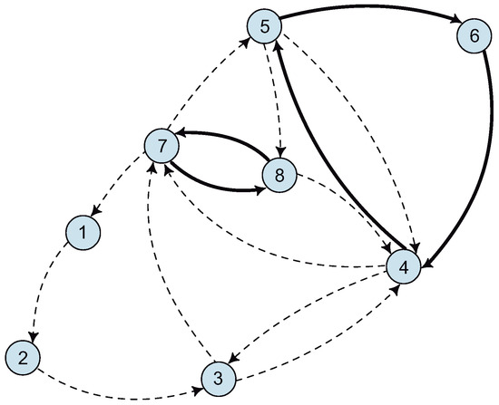
Figure 3.
Compatibility graph of cycle-only KEP with , , and ; the optimal solution is depicted by bold arcs.
In the following developments, let P be the set of patient–donor pairs and let N be the set of non-directed donors. We model the KEP on a directed graph where the set of vertices is partitioned into and . In the absence of NDDs, as is the case with the cycle-only version, . The set of arcs A contains arc if and only if the donor at node i is compatible with the patient in pair j such that . Note that , as NDDs do not have paired patients, and consequently do not have incoming edges. The digraph has no loops, as we assume every PDP is incompatible. Each arc has a weight representing the priority given to that transplant by the transplant center. These weights are used to capture various prioritization schemes and other value judgments. There is a maximum cycle length limit given by k due to logistical issues. The largest chain length is constrained to L; however, L may be long or even unbounded.
When only cycles are considered, the KEP can be modeled as the cycle packing problem on a directed graph [13]. Figure 3 depicts a compatibility graph and an optimal solution when cycles of length at most are allowed and there are no NDDs in the pool. The optimal assignment is shown by bold arcs, while dashed arcs represent original compatible arcs that are not part of the optimal solution. Likewise, Figure 4 depicts the KEP instance presented in Figure 3 with NDDs and its optimal solution when different values of are present.
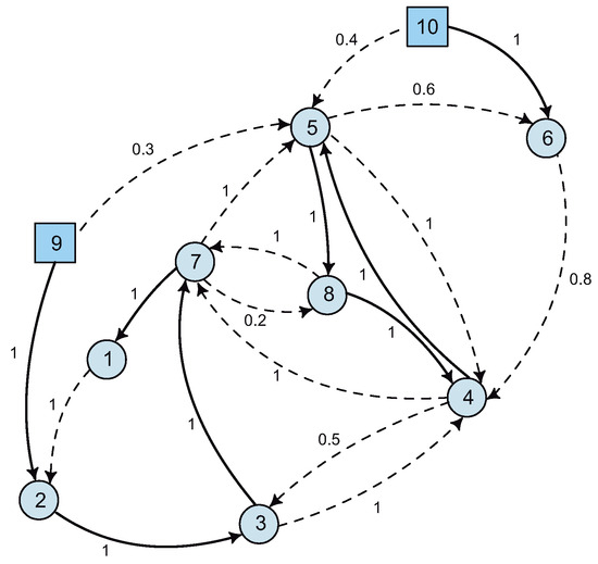
Figure 4.
Compatibility graph of cycle-and-chain KEP with , (square nodes), , arc weight shown along the arc, and l unbounded; the optimal solution is depicted by the bold edges.
4. New Arc-Based Formulations
In this section, we introduce three new formulations, taking as our reference the edge formulation proposed by Abraham et al. [11] and Roth et al. [14]. Our main idea is to extend these formulations by exploiting special graph connectivity properties that allow us to significantly reduce model size.
4.1. Strong Connectivity
From graph theory, we know that a graph G that is not a strongly connected component (SCC) by itself can be partitioned into a collection of vertex-disjoint and edge-disjoint strongly connected subgraphs.
Definition 1.
A strongly connected component of a directed graph G is a maximal subset of vertices such that we have both and for every pair of vertices u and v in S, that is, there is a directed path from u to v and a directed path from v to u.
One property of strong connectivity is that it partitions vertices such that each vertex belongs to exactly one SCC, as stated in the following lemma.
Lemma 1.
In a directed graph, each vertex belongs to exactly one SCC.
Proof.
By contradiction, let us suppose that there is a vertex v belonging to two different strongly connected components in a directed graph , namely, S and . Because , we have for each vertex . Similarly, because , we have for each vertex . It follows that and for every vertex and , that is, , which is a contradiction. Therefore, vertex v belongs to exactly one SCC. □
Note that if there exist any arcs leaving one SCC S and entering another distinct , such arcs will never be part of a cycle, since G does not contain a path from to S that returns to ; otherwise . Figure 5 depicts a graph with four SCCs, two of which can actually form a cycle. In fact, the only component that represents an optimization problem is the one containing nodes {1,2,3,4}, as nodes 6 and 7 clearly form part of the optimal solution for . Therefore, arcs (3,6), (4,5), (6,7), (7,6), (8,5), and (8,7) can be disregarded in any arc-based model without affecting optimality.
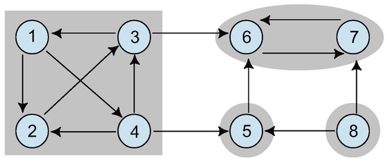
Figure 5.
Examples of SCCs.
There are several classical linear-time algorithms for finding strongly connected components of a digraph, for example Tarjan’s algorithm [41] and Kosaraju-Sharir’s algorithm [42]. Depending on the graph representation, both run in time.
4.2. Partitioned Edge Formulation (*PE)
This formulation addresses the cycle version of the KEP. Given the input graph , let be the set of subgraphs induced by each of the SCCs of G, where q is the number of non-trivial SCCs of G, i.e., SCCs containing nodes with degree greater than zero. We interchangeably refer to as the subgraph or as the SCC in Q. Moreover, let be the full set of paths with length k in subgraph . Thus, we have q optimization subproblems. Now, for each arc , we define a variable such that
The partitioned edge formulation (*PE) can be expressed as follows:
The objective function (1) maximizes the weighted sum of matches. In the case of unit weights, it maximizes the total number of transplants. Constraints (2) guarantee that donor i provides a kidney if and only if patient i receives one in return. Constraints (3) ensure that a person can only donate a single kidney, and constraints (4) enforce the requirement that the length of any cycle must be less than or equal to k. Any feasible cycle will always contain a path with at most arcs (no repeating arcs). Therefore, if we preclude all paths of length k from being part of a cycle, then cycles of length or greater will also be excluded from a feasible solution.
Model *PE looks like the edge formulation [11,14] referred to as formulation E in Section 6.3, yet it has significant differences. It is applied independently to each SCC in Q; thus, optimizing over G is reached by optimizing over each subgraph . Note that here represents a subset of all the k-length paths of G, referred to as in the edge formulation. Moreover, we show that the upper bound provided by linear relaxation of (1)–(5) is at least as good as that obtained by formulation E in Section 4.5. This follows because paths of length k that are not contained in , i.e., paths emerging and ending at different SCCs, do not constrain the size of any cycle. As shown before, this is because a cycle does not exist among different SCCs. In the edge formulation, the set can be replaced by without altering the correctness of the model.
4.3. Partitioned and Reduced Edge Formulation (*PRE)
This formulation represents the cycle-only version of the KEP. The partitioned edge formulation significantly reduces the number of constraints; however, when graph G is itself a SCC, it turns into the edge formulation. In this section, we propose a new formulation for general graphs.
4.3.1. SCC-Based Search for Length-k Paths
The first important observation is that the number of paths of length k (in terms of arcs) that is present under the edge or reduced edge formulation is larger than the number of infeasible cycles (simple cycles of length greater than k) to be ruled out. For instance, assuming , for an infeasible cycle of length 4 formed by nodes , there are four different directed paths of length 3 in , each starting at a different node in cycle C. Naturally, three of them are not needed and may be omitted from the formulation without altering the optimal solution. Under this reasoning, each infeasible cycle accounts for as many path constraints as the number of nodes in it.
To explain the algorithm, we consider two different types of k-length paths: (i) a critical k-length path is a path that could lead to a cycle of length if an arc was added; (ii) a non-critical k-length path is the opposite, that is, one where no cycle of length or more can be formed by adding an arc to it. For instance, the path in Figure 3 is a critical path because adding an arc forms a cycle of length 4. In contrast, the path is non-critical because no cycle of length 4 can be formed from it by adding any arc.
Given the small size of this example, it is easy to identify the non-critical paths; however, this is not the case in a large graph. The essence of our approach is to provide a clever way of identifying non-critical paths while keeping only those that are needed for ruling out infeasible cycles.
Algorithm 1 formally defines the process just described. The algorithm takes as input the directed graph G, then finds both and its set of length-k paths . Note that is the full set of paths of length k for component , whereas is the subset of for which the cardinality constraints over the cycles are satisfied.
| Algorithm 1 SCC-based search for finding paths of length k in a KEP graph |
|
Let be a procedure that finds the non-trivial SCCs in a directed graph G. Here, we use the Kosaraju-Sharir algorithm [42]. Let be a collection of SCCs from which the next SCC T is chosen to find its length-k paths. Every time the SCCs are recomputed for a given component T, a new collection of SCCs is obtained and added to . Let be the set of arcs that are incident to u.
Additionally, let be a procedure for finding a node in T to remove. The node to be removed depends on the node selection strategy provided by “g”, where g∈ {in-degree, out-degree, total degree}; e.g., returns the node in T with highest out-degree. Ties are broken arbitrarily. Let be the well-known algorithm for traversing graph data structures by starting at node u and traverses T in the search for paths of length k, then returning the set of length-k paths starting at node u. In addition, let be a function that returns the subgraph in with the largest cardinality node set.
To illustrate the algorithm and its underlying concepts, we can consider the graph in Figure 3 with (that is, allowing only cycles of length k or less). In arc-based models, one way of eliminating cycles of length or more is to use path-based cycle-elimination constraints, as in (4). There, the authors established that if a k-length path can only use arcs, then there cannot be cycles of length or more, because adding an arc to the path in order to form a cycle would increase its length from k to . Such path-based cycle elimination constraints have been used previously [11,14].
In our example, there are nine infeasible cycles (of length 4 or more) provided by . Table 1 displays the full set of length-3 paths when using k-length paths for cycle elimination.

Table 1.
Full set of length-3 paths for Figure 3. A star (*) indicates a critical path.
The importance of distinguishing critical and non-critical paths is that path-based cycle elimination constraints imposed to prevent cycles of length or more should be imposed over critical paths only; in other words, it is not necessary to impose path-based cycle elimination constraints on non-critical paths. In Table 1, the critical paths are indicated with a star (*) at the end. Naturally, we do not know in advance what the critical and non-critical paths are; rather, the idea is to use the fewest possible path-based cycle elimination constraints by ensuring that all constraints are associated with critical paths while also using the fewest possible constraints associated with non-critical paths.
If we choose an arbitrary node, say, node 4, and identify all length-k constraints starting at this node (which would eliminate all infeasible cycles associated with node 4), then any infeasible cycle will not contain node 4. Therefore, node 4 can be removed from the graph, and apply the same reasoning can be applied to the remaining graph. By pursuing this strategy one node at a time in an iterative way, we end up generating constraints that prevent all infeasible cycles. This is precisely the main idea of the algorithm.
Figure 6 shows the steps of the algorithm for this particular example. In quadrant I, node 4 is arbitrarily chosen, giving rise to seven length-3 paths (identified by different markers on the arcs). In quadrant II, after removing node 4, two new SCCs remain (the shaded areas). One of them is a trivial single-node SCC and the other is a new subgraph. Quadrant III shows the next iteration of the algorithm, where an arbitrary node is chosen (in this case node 7) and its length-3 paths are generated (only one path in this case). In quadrant IV, the SCCs are recomputed after removing node 7; however, this time we obtain six trivial components (one node each), because the nodes are not mutually reachable from each other as stated in Definition 1.
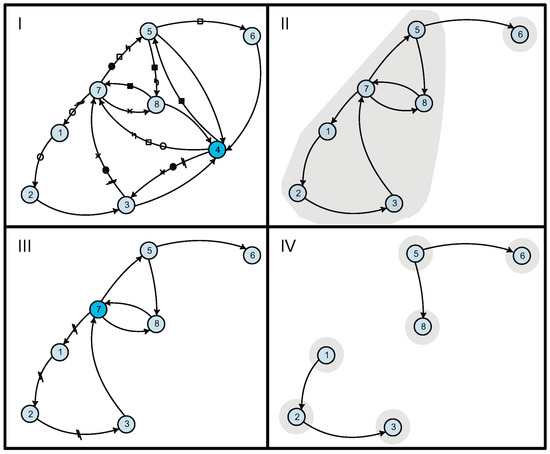
Figure 6.
Sequentially removing a vertex from a strongly connected component.
At this point, the process ends because no more strongly connected components with more than k nodes remain in the graph. Thus, we have found eight length-3 paths, as identified in Table 2. We can observe that the selected nodes are included in any collection of feasible cycles in the graph, along with the ones contained in the remaining non-trivial strong components (with at most k nodes). As such, the process not only obtains a significant reduction in the number of length-k paths, it also finds an upper bound on the number of cycles in a solution as well as the nodes that are necessarily included in them.
Table 2.
Set of length-3 paths obtained using the SCC-based search for Figure 3.
As shown in this example, one important aspect of the iterative process is choosing the node u to be removed. In this regard, three different node selection rules were tested: choosing the node with (a) the maximum in-degree, (b) the maximum out-degree, and (c) the maximum total degree. In general, the maximum in-degree rule produced the best results, with a larger number of paths eliminated under this rule compared to the others. This can be explained in part by noting that the number of paths increases with the number of outgoing arcs from the selected node u, at least empirically. When picking the node with highest in-degree instead, the number of outgoing arcs is generally smaller, meaning that fewer paths are obtained. Thus, a large number of cycles is discarded when using a smaller number of paths.
4.3.2. Tournament Inequalities
Ascheuer et al. [43] proposed the use of tournament inequalities for the asymmetric traveling salesman problem, which has been shown by Mak-Hau [17] to be valid and facet-defining for the cycle-only version of the KEP. In this section, we show the strength of these constraints compared to the infeasible cycle elimination constraints of the classical edge formulation.
Consider the following length-k path and its associated constraint:
The well known idea behind Constraint (6) is to break a path with nodes (k arcs) such that at most of its arcs are used to form a valid cycle. Otherwise, the path with k arcs would lead to an infeasible cycle. By using one or more arcs not included in (6) alongside these edges, cycles with cardinality less than or equal to k can be obtained. Note that a subset of the nodes in path can form several sub-paths if the corresponding arcs exist in the original graph; i.e., paths such as or may also exist. In addition, we can observe that the flow-balance constraints in (9) allow only one such path or set of sub-paths. Because all of them will collectively contain at most arcs, the following set of constraints is valid for the KEP:
where .
Only sub-paths flowing in one direction, e.g., from lower to higher node indices, need be taken into account to guarantee that the left-hand side of (7) only yields paths. We now replace the constraints in (4) with the tighter set in (7). To understand the value of these inequalities, we again consider the graph in Figure 3. In the path 4 → 7 →5 → 6, there exists a sub-path 4 → 5 → 6. If , then the new associated constraint is . Now, consider the fractional solution and , which is feasible for constraints (4), namely, , but not for constraints (7), which cuts off this fractional solution and rules out its associated infeasible cycle 4 → 7 →5 → 6 → 4.
The Partitioned and Reduced Edge (*PRE) formulation is then provided as follows:
4.4. The Reduced Exponential-Sized SPLIT Formulation (*ReSPLIT)
This formulation addresses the cycle-and-chain version of the KEP. A natural extension of the exponential-size SPLIT formulation by Mak-Hau [16] is to replace constraints of the type
in the SPLIT model from Mak-Hau [16], with the constraints in (11). Using Algorithm (1), we aim to find a small subset of k-length paths instead of the full set while also maintaining model correctness. When the graph is partitioned into its SCCs, some arcs are removed. This results in feasible paths being lost, potentially including the optimal solution. Therefore, we cannot solve each SCC separately, since we now have to find a collection of node and arc disjoint paths.
4.5. Model Properties
Given two integer programming formulations and with the same objective function for an optimization problem, we say that dominates if the feasible region of the linear programming relaxation of is a subset of the feasible region of the linear programming relaxation of . The strength of the Linear Programming (LP) relaxation is used as a performance measure in LP-based solution methods such as branch and bound.
Lemma 2.
Lemma 3.
The cycle formulation [11,14] dominates the extended edge formulation [15].
Lemma 4.
The same proof provided with regard to the cycle and edge formulation in [11] can be used to prove Lemma 2. The proofs for Lemmas 3 and 4 are provided by Constantino et al. [15]. Although neither the partitioned edge formulation nor the partitioned and reduced edge formulation are compared explicitly in [15], the same reasoning used in the other comparisons can be applied.
5. Solution Algorithms
All the existing and proposed formulations presented in Table 3 and in the previous sections were solved with CPLEX. However, there are some variations in the solution algorithms due to the exponential number of cardinality constraints in some models. In this section, we provide details about the solution algorithms for the new formulations.
Table 3.
Notation used to reference KEP formulations.
5.1. The *PE Formulation
The solution algorithm for the *PE formulation consists of two steps. First, the strongly connected components with associated k-length paths are found, that is, subsets for each are identified. Then, the corresponding path-elimination constraints (4) are generated. The resulting *PE model (1)–(5) is fed to the solver to obtain the optimal solution. There are several algorithms in the literature for finding strong components and simple paths, several of which are mentioned in Section 4.3. In this study, whenever it was necessary to find the strongly connected components and the full set of length-k paths, we used the Kosaraju-Sharir algorithm [42] and a depth-first search procedure, respectively.
5.2. The *PRE and *ReSPLIT Formulations
After finding the cardinality constraints with Algorithm 1, the next step is to solve both the *PRE and the *ReSPLIT models. For the former, there are as many subproblems as the number of strongly connected components of , just as in the case of the *PE formulation. For the latter, the entire instance is optimized using the length-k paths contained in . Because the *ReSPLIT formulation finds cycles and chains, it is not possible to solve each subproblem separately.
Before optimizing either model, we preprocess the graphs by removing all length-k paths that do not lead to a feasible cycle. In Section 4.3, we have shown that some paths in a strongly connected component may be part of a circuit, meaning that there is no need to constraint them. Moreover, even if a path forms a simple cycle, it may be infeasible. If an arc belonging to a path in does not lead to a feasible cycle, i.e., if it is only part of a circuit or infeasible simple cycle, then we remove the arc (this is done for the cycle version only) and the path from and , respectively. Finally, we recompute the strongly connected components of . If we obtain new separate components by this procedure, then we will have as many subproblems as the number of new strong components, instead of only the one represented by . Recall from Section 4.2 that , are the original strongly connected components of graph G. This increase in the number of subproblems resulting from the decomposition is especially useful for hard-to-solve instances.
Now, we formally introduce the procedure outlined above. Let be the subgraph represented by and let be a path in . In addition, let represent the set of new strongly connected components after removing redundant arcs from and let represent the updated set of length-k paths after removing non-necessary paths. Lastly, let be the set of length-k paths leading to a feasible cycle in subgraph . A depth-first search starting from each arc is performed to determine whether an arc belongs to . If the same arc is included in multiple paths, then the depth-first search is performed only once for that arc. The procedure is shown in Algorithm 2 and has complexity [44]. After updating the number of subproblems and paths, we proceed to solve both formulations.
| Algorithm 2 Removing unnecessary arcs and paths in subgraph |
|
6. Results
6.1. Description of Database Instances
The instances used to test our new formulations were taken from Anderson et al. [8], who simulated the National Kidney Registry (NKR) pool over a two-year period from 24 May 2010 to 24 May 2012. The initial pool contained 63 patient–donor pairs, while an additional 410 pairs registered over the course of the study. The dataset also contained 75 altruistic donors. Compatibility between donors and patients was determined primarily by blood type and human leukocyte antigen compatibility rules, although some patient preferences were also taken into account.
To create representative snapshots of actual instances encountered by a kidney-paired donation program, the authors considered the fact that easy-to-match patients tend to wait only a short time before being selected, leaving hard-to-match patients in the pool after each match run. Overall, the graph density of these instances is low, being less than or equal to 20%. For full details, see Anderson et al. [8] and Anderson [45].
6.2. Experimental Conditions
In the remainder of this section, we discuss the computational experiments designed to compare existing formulations with our new formulations regarding runtime and solution quality (when an optimal solution was not found). All models were either solved directly with CPLEX 12.7 using Concert Technology (Sterling, VA, USA) or with a specialized method on a PC with an Intel Core i7 processor running at 3.40 GHz and 8 Gb of RAM. In general, all models were coded using C++ and a time limit of 1800 s was placed on all runs.
The computational analysis was performed as follows. First, ten instances were grouped into each trial set, sorted in non-decreasing order of the average number of PDPs for the both cycle-variant formulations and the cycle-and-chain formulations. The maximum cycle length we considered was , and no bound was placed on the length of the chains. The original instances include NDDs; in order to test the cycle-variant formulations, we dropped the nodes and arcs associated with the NDDs. All cycle-variant formulations were tested for all instances. For the cycle-and-chain formulations, we first tested all instances with and , then took the two best performers and compared them for and . The objective function for all models was the weighted sum of arcs.
6.3. Description of Comparison Algorithms
Table 3 lists each formulation, its abbreviation, the reference, and the KEP variant. The IP formulations in the literature that include chains and cycles generally do not include upper bounds on the chain lengths. Similarly, we did not consider bounded chains. In the table, the argument “i” in *PRE(i) and *ReSPLIT(i) refers to the maximum in-degree node selection strategy used by the SCC-based search algorithm to find the length-K paths for each formulation. Because the maximum out-degree and maximum degree strategies yielded a larger number of paths, we only present results for the in-degree node selection strategy discussed in Section 4.3.
6.4. Evaluation Metrics
When presenting the output statistics, we make use of the following notation:
- PDPsR: Range for the number of PDPs after grouping ten instances in non-decreasing order of PDPs. This value is represented by an interval [b,u], written as b-u in the output tables, where b(u) represents the smallest (largest) number of PDPs found in the specific subset.
- NDDsR: Interval for the number of NDDs after grouping the instances into sets of ten in non-decreasing order of PDPs. Again, this value is represented by an interval b-u, where b(u) represents the smallest (largest) number of NDDs found in the specific subset.
- *PRE(i): Partitioned and reduced edge formulation when the node selection strategy for the SCC-based search algorithm uses the maximum in-degree.
- nf: Number of subproblems that failed to obtain a feasible solution, either because CPLEX was unable to solve the initial LP relaxation after the time limit or because CPLEX displayed an out-of-memory status before the start of branching. The notation () indicates that there were and instances in which no feasible solutions were found because of the former and latter cases, respectively.
- aVars: Average number of variables in a formulation for a subset of instances.
- saVars: Relative decrease in the number of variables passing from the edge formulation to the *PE or *PRE(i) formulations. The former is provided bywhere n stands for the total number of instances, e.g., , and () is the number of variables for instance j obtained by using the E (*PE or *PRE(i)) formulation.
- aCons: Average number of constraints for a set of instances. In the case of the AA and the PC-TSP formulations, the violated lazy constraints added throughout the solution process are included.
- saCons: Relative decrease in the number of constraints passing from the edge formulation to the *PE or *PRE(i) formulations. The former is provided bywhere () is the number of constraints for instance j obtained by using the E (*PE or *PRE(i)) formulation.
- nSCC: Average number of strongly connected components (subproblems) in which the graphs of each set of instances are split into their separate components.
- SCCp(i): Average number of constraints for a set of instances of the *PRE(i) formulation before preprocessing (discussed in Section 5.2), and using the maximum in-degree strategy in Algorithm 1.
- sSCCp(i): Relative decrease in the number of constraints passing from the edge formulation to the *PRE(i) formulation before preprocessing, provided by the expressionwhere is the number of constraints for instance j obtained by using the *PRE(i) formulation before preprocessing.
- tc and tp: Time to find feasible cycles in order to determine the variables needed in the cycle formulation and time to find length-K paths in each formulation, respectively. To search for feasible cycles, we implemented an adaptation of Johnson’s algorithm [46].
- tsep: Average time needed to find and add all the violated lazy constraints to the AA and PC-TSP formulations.
- tr: Average time needed to perform the preprocessing step (discussed in Section 5.2).
- time: Average runtime in seconds to reach the best feasible solution for a set of instances. The runtime limit was set to 1800 s for all formulations. Note that the *PE and *PRE formulations split the original problem into independent subproblems; thus, the times reported for those formulations are the sum of times for all subproblems.
- opt: Number of instances solved to optimality. In all cases, the objective function is the weighted arc sum. Whenever this column does not appear in the output tables, it is because all instances were solved to optimality.
- gap: Average relative optimality gap associated with a formulation, defined by , where is the upper bound provided by the linear relaxation of the formulation and is either the optimal value, or the best lower bound that could be found when the optimal value was unknown. This column does not appear when all instances were solved to optimality.
The solution algorithms for the proposed formulations are discussed in Section 5. A discussion on how the existing formulations are solved is provided in Riascos Alvarez [44].
6.5. Assessment of Cycle-Variant Formulations
This subsection presents results for the cycle-only formulations. Table 4 highlights the comparisons for 3-way cycles, that is, for . Each row represents average findings for a subset of instances (as indicated in the first column). Although most instances turned out to be “easy” for all the formulations tested, the C, rEE, and *PRE(i) formulations show dominance over the E and *PE formulations because they were able to optimally solve all instances in less time on average. Summing the time for preprocessing, searching for paths, and finding the solution, the *PRE(i) and rEE formulations have comparable performance for most sets of instances. The increase in runtimes for the first and last set of instances is related to the number of length-3 paths in some subproblems. In contrast, in any set of instances there are graphs that can be partitioned into several subgraphs, giving an extra advantage to the *PE formulation over the E formulation. In addition, it should be noted that the preprocessing procedure for the *PRE(i) formulation is not computationally expensive. The E formulation performed fairly well, but memory ran out in two instances in the last dataset.
Table 4.
Comparison of formulations for 3-way cyclic exchanges.
Table 5 shows the results for 4-way cyclic exchanges. The dominance of the C, rEE, and *PRE(i) formulations is clear in terms of both runtime and number of optimal solutions found in comparison to the E and *PE formulations. In the last set of instances, however, the *PRE(i) formulation did not perform as well as the C and rEE formulations with regard to the runtime results, although they were still reasonable.
Table 5.
Comparison of formulations for 4-way cyclic exchanges.
Table 6 and Table 7 analyze the input size of the instances for all formulations as well as the percentage reduction in the number of variables and constraints for the *PE and *PRE(i) formulations before and after the reduction procedure described in Section 5. The first observation is that the input size of the C formulation is the smallest for all sets of instances, which explains its outstanding performance. The second is the huge reduction in the number of variables and constraints for the *PE and *PRE(i) formulations. This is especially true for the latter, reaching savings of more than 85% and 99% in the number of variables and paths, respectively. These results demonstrate the benefits of using our approach for reducing the number of length-k paths for an arc-based formulation when and . For the tested instances, the number of paths of length k seems to increase as k increases, and in some sets of instances as the number of PDPs increases as well.
Table 6.
Size of formulations for 3-way cyclic exchanges.
Table 7.
Size of formulations for 4-way cyclic exchanges.
However, it is worth noting that the SSC-based search algorithm was particularly successful because the compatibility graphs of the kidney exchange pool were sparse. If the graph is complete and has n nodes, the time complexity of our algorithm is . We never saw runtimes approaching this value for the tested instances, as the number of paths of length k seemed to increase linearly with n for (column SCCp in Table 6) and with for (column SCCp in Table 7).
6.6. Assessment of Cycle-and-Chain Variant Formulations
This subsection evaluates the performance of the different variants of the cycle-and-chain formulations. The one exception is the eSPLIT formulation, which is omitted because its cycle variant, the edge formulation (E), exhibited the worst performance in the first set of experiments discussed in the previous section, as evidenced by the largest runtimes and greatest number of failures due to memory overload.
Table 8 reports the results for 3-way cyclic exchanges and unbounded chains for the remaining formulations. As can be seen, the KEP now becomes harder to solve. With respect to our performance measures, the pSPLIT and *ReSPLIT(i) formulations dominate the AA and PC-TSP formulations in terms of runtime and number of optimal solutions found. Except for the last set of instances, the statistics for the pSPLIT and *ReSPLIT(i) formulations are practically the same.
Table 8.
Comparison of formulations for 3-way cyclic exchanges and unbounded chains.
The solution algorithm is fully described in Riascos Alvarez [44]. Essentially, exponential constraints of the type for , are initially dropped from the AA and PC-TSP models and only added back if they are violated when B&B finds an integer solution. The model is then reoptimized in an iterative fashion. Note that if the integer solution found after reaching the time limit still violates some cardinality constraints, i.e., if additional constraints are still needed, then that solution is deemed infeasible. Under this algorithm, the solutions for the AA and PC-TSP formulations are either optimal or infeasible; thus, the gap columns are omitted in Table 8.
Anderson et al. [8] compared the AA and PC-TSP formulations using a lazy-constraint and a branch-and-cut approach, respectively, on a set of “difficult” instances. Ten of those instances are included in our eight datasets. Table 9 compares the results obtained in Table 8 with our two cycle-and-chain variant formulations. As can be seen, the pSPLIT and *ReSPLIT formulations, both of which also use a lazy constraint approach, outperform the AA and PC-TSP formulations. In addition, a comparison of the results obtained with the pSPLIT and *ReSPLIT formulations shows little difference with respect to runtimes, gaps, and number of optimal solutions. On the other hand, the AA formulation is superior to the PC-TSP formulation for all instances tested, identifying a greater number of optimal solutions in less time.
Table 9.
Comparison of instances in [8] with 3-way cyclic exchanges and unbounded chains.
Table 10 shows the runtimes, gaps, and number of optimal solutions reached by the pSPLIT and *ReSPLIT formulations when and . The performance of both formulations is again very similar, except for the last set of instances, where CPLEX could not find an integer solution within the 1800-s time limit for two subproblems associated with one instance each under the *ReSPLIT(i) formulation. This behavior can be explained in part by analyzing the statistics in Table 11 and Table 12. For both formulations, the size of the instances is roughly the same except for the last dataset, where there is a sharp increase in the number of constraints for the *PRE(i) formulation, especially when .
Table 10.
Comparison of formulations for 4-way cyclic exchanges and unbounded chains.
Table 11.
Size of formulations for 3-way cyclic exchanges and unbounded chains.
Table 12.
Size of formulations for 4-way cyclic exchanges and unbounded chains.
7. Summary and Conclusions
7.1. Main Findings
This paper presents three new formulations for the Kidney Exchange Problem: (1) the partitioned edge formulation (*PE); (2) the partitioned and reduced edge formulation (*PRE); and (3) the reduced exponential-sized SPLIT formulation (*ReSPLIT), which are empirically shown to be superior to the well-known edge formulation. An algorithm for reducing the number of paths of length k is proposed, representing the first reported attempt to do so for an edge-based formulation. Dominance proofs are provided for the cycle-variant formulations studied, and extensive computational tests are performed to compare the solution quality, runtimes, and related statistics obtained for the existing and new formulations.
Regarding the cycle-variant formulations, our computational results confirm that the cycle formulation (C) is very effective for low-density graphs, outperforming the other cycle-variants we tested. The standard edge formulation is shown to be relatively ineffective for solving any instances, and grows substantially worse as k increases. The partitioned edge formulation outperforms the edge formulation, but only when the graphs are not a unique strongly connected component. As we know, non-compact formulations tend to perform poorly when k becomes large or when graphs have higher density. In such cases, compact formulations perform better [15]. Very good results were obtained when comparing our model with compact formulations such as the extended edge (rEE) formulation.
The *PRE(i) formulation uses a new set of constraints and a small subset of the full set of length-k paths that are included in the edge formulation. The reduction in the number of such paths is greater than 98% for all tested instances. The performance of the *PRE(i) formulation is very similar to that of the extended edge formulation, although the latter performs better on the largest instances and when .
With respect to the cycle-and-chain formulations, the extensions of the exponential-sized SPLIT formulation (*ReSPLIT) outperformed Anderson’s arc-based formulation and the PC-TSP formulation on all tested instances. In particular, when tested on the set of “difficult” instances from Anderson et al. [8], our proposed *ReSPLIT model provided the best results compared to the AA and PC-based models solved by a lazy-constraint algorithm.
7.2. Discussion of Future Work
The most successful computational work for the KEP has been performed within the branch-and-price framework, as arc formulations with an exponential number of constraints have proven unsolvable with commercial software even for small instances. As indicated in the literature review section, there are two types of KEP models, namely, those based on an exponential number of variables and those based on an exponential number of constraints. For the former, column generation and branch-and-price approaches have been developed with a certain degree of success. For the latter, existing models have again proven unsolvable with commercial software even for relatively small instances. Thus, it could be worthwhile to investigate how the models proposed in this work might be used within such column generation schemes.
To date, the constraint generation approach in [8] remains the only known approach for tackling the cycle-and-chain setting. However, it is only competitive when the cycle length is 3 and the chain length is unbounded. Therefore, an interesting avenue for future research could involve the use of polyhedral theory to develop branch-and-cut algorithms for the partitioned and reduced edge formulation. In this study, we have proposed a heuristic for reducing the exponential number of path elimination constraints while ensuring optimality; however, only “static” strategies were considered when selecting the node to be removed. A deeper examination of the problem structure might lead to more tailored strategies and strong valid inequalities that would improve the upper bound provided by LP relaxation. Another line of research could be to extend the present work in order to handle dynamic or stochastic cases. In the past few years, a few stochastic [24,29,30] and dynamic [37] kidney exchange models have been developed. It would be interesting to study how the algorithmic ideas developed in this paper could be applied to those cases.
Today, the complexity and size of real instances in many countries are still manageable using the most efficient exact methods reported in the literature. However, as KEP programs and countries continue to look into ways of sharing databases, this could result in large-scale instances that are likely to be intractable with exact methods. This opens the door for other non-exact methods, such as heuristics, metaheuristics, matheuristics, and deep reinforcement learning, to name a few.
Author Contributions
L.C.R.-Á.: Methodology, Software, Validation, Formal analysis, Investigation, Data Curation, Writing–Original Draft, Visualization; R.Z.R.-M.: Conceptualization, Methodology, Validation, Formal analysis, Resources, Writing–Original Draft, Supervision, Project administration, Funding acquisition; J.F.B.: Validation, Resources, Writing–Original Draft, Conceptualization, Methodology, Validation, Formal analysis, Resources, Writing–Original Draft, Supervision. All authors have read and agreed to the published version of the manuscript.
Funding
The first author was funded by the Mexican Council for Science and Technology (CONACyT), grant CF-2023-I-880, and by Universidad Autónoma de Nuevo León through its Scientific and Technological Research Support Program, grants CE876-19, CE1416-20, CE1837-21, and 241-CE-2022. The second author was financially supported by a scholarship for graduate studies from the CONACyT. The APC was funded by MDPI.
Data Availability Statement
Some data is proprietary; however, sharable data is available from the authors upon request.
Acknowledgments
We are grateful to four anonymous reviewers whose criticism helped to improve the presentation of this work. Additionally, we would like to thank Ross Anderson, Itai Ashlagi, and Alvin Roth for kindly sharing their test instances with us and for the helpful comments. We also acknowledge enlightening discussions with John Dickerson about kidney exchanges.
Conflicts of Interest
We declare that we do not have any conflict of interest with any of our funding agencies. The funding agencies have been listed in the online system. Our research does not involve human participants and/or animals. All co-authors have agreed to submit the manuscript to the journal. The findings have not been published elsewhere. The manuscript is not currently under consideration by another journal. The datasets generated during the current study are not publicly available due to proprietary reasons, but are available from the corresponding author on reasonable request.
References
- Ross, L.F.; Rubin, D.T.; Siegler, M.; Josephson, M.A.; Thistlethwaite, J.R.; Woodle, E.S. Ethics of a paired-kidney exchange program. N. Engl. J. Med. 1997, 336, 1752–1755. [Google Scholar] [CrossRef] [PubMed]
- Delmonico, F.L. Exchanging kidneys—Advances in living-donor transplantation. N. Engl. J. Med. 2004, 350, 1812–1814. [Google Scholar] [CrossRef] [PubMed]
- Roth, A.E.; Sönmez, T.; Ünver, M.U. Kidney exchange. Q. J. Econ. 2004, 119, 457–488. [Google Scholar] [CrossRef]
- Roth, A.E.; Sönmez, T.; Ünver, M.U. Pairwise kidney exchange. J. Econ. Theory 2005, 125, 151–188. [Google Scholar] [CrossRef]
- Roth, A.E.; Sönmez, T.; Ünver, M.U. A kidney exchange clearinghouse in New England. Am. Econ. Rev. 2005, 95, 376–380. [Google Scholar] [CrossRef]
- Anderson, R.; Ashlagi, I.; Gamarnik, D.; Rees, M.; Roth, A.E.; Sönmez, T.; Ünver, M.U. Kidney exchange and the alliance for paired donation: Operations research changes the way kidneys are transplanted. Interfaces 2015, 45, 26–42. [Google Scholar] [CrossRef]
- Gentry, S.E.; Montgomery, R.A.; Swihart, B.J.; Segev, D.L. The roles of dominos and nonsimultaneous chains in kidney paired donation. Am. J. Transplant. 2009, 9, 1330–1336. [Google Scholar] [CrossRef]
- Anderson, R.; Ashlagi, I.; Gamarnik, D.; Roth, A.E. Finding long chains in kidney exchange using the traveling salesman problem. Proc. Natl. Acad. Sci. USA 2015, 112, 663–668. [Google Scholar] [CrossRef]
- Ashlagi, I.; Gilchrist, D.S.; Roth, A.E.; Rees, M.A. Nonsimultaneous chains and dominos in kidney-paired donation—Revisited. Am. J. Transplant. 2011, 11, 984–994. [Google Scholar] [CrossRef]
- Dickerson, J.P.; Procaccia, A.D.; Sandholm, T. Optimizing kidney exchange with transplant chains: Theory and reality. In Proceedings of the 11th International Conference on Autonomous Agents and Multiagent Systems (AAMAS’12), Volume 2, Valencia, Spain, 4–8 June 2012; International Foundation for Autonomous Agents and Multiagent System: Richland, SC, USA, 2012; pp. 711–718. [Google Scholar]
- Abraham, D.J.; Blum, A.; Sandholm, T. Clearing algorithms for barter exchange markets: Enabling nationwide kidney exchanges. In Proceedings of the 8th ACM Conference on Electronic Commerce, San Diego, CA, USA, 11–15 June 2007; pp. 295–304. [Google Scholar]
- Edmonds, J. Paths, trees, and flowers. Can. J. Math. 1965, 17, 449–467. [Google Scholar] [CrossRef]
- Biró, P.; Manlove, D.F.; Rizzi, R. Maximum weight cycle packing in directed graphs, with application to kidney exchange programs. Discret. Math. Algorithms Appl. 2009, 1, 499–517. [Google Scholar] [CrossRef]
- Roth, A.E.; Sönmez, T.; Ünver, M.U. Efficient kidney exchange: Coincidence of wants in markets with compatibility-based preferences. Am. Econ. Rev. 2007, 97, 828–851. [Google Scholar] [CrossRef] [PubMed]
- Constantino, M.; Klimentova, X.; Viana, A.; Rais, A. New insights on integer-programming models for the kidney exchange problem. Eur. J. Oper. Res. 2013, 231, 57–68. [Google Scholar] [CrossRef]
- Mak-Hau, V. On the kidney exchange problem: Cardinality constrained cycle and chain problems on directed graphs: A survey of integer programming approaches. J. Comb. Optim. 2017, 33, 35–59. [Google Scholar] [CrossRef]
- Mak-Hau, V. A polyhedral study of the cardinality constrained multi-cycle and multi-chain problem on directed graphs. Comput. Oper. Res. 2018, 99, 13–26. [Google Scholar] [CrossRef]
- Lam, E.; Mak-Hau, V. Branch-and-cut-and-price for the cardinality-constrained multi-cycle problem in kidney exchange. Comput. Oper. Res. 2020, 115, 104852. [Google Scholar] [CrossRef]
- Rapaport, F.T. The case for a living emotionally related international kidney donor exchange registry. Transplant. Proc. 1986, 18, 5–9. [Google Scholar]
- Ross, L.F.; Woodle, E.S. Ethical issues in increasing living kidney donations by expanding kidney paired exchange programs. Transplantation 2000, 69, 1539–1543. [Google Scholar] [CrossRef]
- Roth, A.E.; Sönmez, T.; Ünver, M.U.; Delmonico, F.L.; Saidman, S.L. Utilizing list exchange and nondirected donation through ‘chain’ paired kidney donations. Am. J. Transplant. 2006, 6, 2694–2705. [Google Scholar] [CrossRef]
- Saidman, S.L.; Roth, A.E.; Sönmez, T.; Ünver, M.U.; Delmonico, F.L. Increasing the opportunity of live kidney donation by matching for two- and three-way exchanges. Transplantation 2006, 81, 773–782. [Google Scholar] [CrossRef]
- Dickerson, J.P.; Manlove, D.F.; Plaut, B.; Sandholm, T.; Trimble, J. Position-indexed formulations for kidney exchange. In Proceedings of the 2016 ACM Conference on Economics and Computation (EC’16), Maastricht, The Netherlands, 24–28 July 2016; ACM: New York, NY, USA, 2016; pp. 25–42. [Google Scholar]
- Alvelos, F.; Klimentova, X.; Viana, A. Maximizing the expected number of transplants in kidney exchange programs with branch-and-price. Ann. Oper. Res. 2019, 272, 429–444. [Google Scholar] [CrossRef]
- Plaut, B.; Dickerson, J.P.; Sandholm, T. Fast optimal clearing of capped-chain barter exchanges. In Proceedings of the Thirtieth AAAI Conference on Artificial Intelligence, Phoenix, AZ, USA, 12–17 February 2016; AAAI Press: Phoenix, AZ, USA, 2016; pp. 601–607. [Google Scholar]
- Glorie, K.M.; Klundert, J.J.v.; Wagelmans, A.P.M. Kidney exchange with long chains: An efficient pricing algorithm for clearing barter exchanges with branch-and-price. Manuf. Serv. Oper. Manag. 2014, 16, 498–512. [Google Scholar] [CrossRef]
- Riascos-Álvarez, L.C.; Bodur, M.; Aleman, D.M. A branch-and-price algorithm enhanced by decision diagrams for the kidney exchange problem. Manuf. Serv. Oper. Manag. 2023, 26, 485–499. [Google Scholar] [CrossRef]
- Arslan, A.N.; Omer, J.; Yan, F. KidneyExchange.jl: A Julia package for solving the kidney exchange problem with branch-and-price. Math. Program. Comput. 2024, 16, 151–184. [Google Scholar] [CrossRef]
- Dickerson, J.P.; Procaccia, A.D.; Sandholm, T. Failure-aware kidney exchange. Manag. Sci. 2019, 65, 1768–1791. [Google Scholar] [CrossRef]
- Pedroso, J.P. Maximizing expectation on vertex-disjoint cycle packing. In Computational Science and Its Applications—ICCSA 2014, Part II; Volume 8580 of Lecture Notes in Computer Science; Murgante, B., Misra, S., Rocha, A.M.A.C., Torre, C., Rocha, J.G., Falcão, M.I., Taniar, D., Apduhan, B.O., Gervasi, O., Eds.; Springer: Cham, Switzerland, 2014; pp. 32–46. [Google Scholar]
- Manlove, D.F.; O’Malley, G. Paired and altruistic kidney donation in the UK: Algorithms and experimentation. Acm J. Exp. Algorithmics 2014, 19, 2.6:1–2.6:21. [Google Scholar] [CrossRef]
- Klimentova, X.; Biró, P.; Viana, A.; Costa, V.; Pedroso, J.P. Novel integer programming models for the stable kidney exchange problem. Eur. J. Oper. Res. 2023, 307, 1391–1407. [Google Scholar] [CrossRef]
- Gentry, S.E.; Segev, D.L.; Simmerling, M.; Montgomery, R.A. Expanding kidney paired donation through participation by compatible pairs. Am. J. Transplant. 2007, 7, 2361–2370. [Google Scholar] [CrossRef]
- Dickerson, J.P.; Kazachkov, A.M.; Procaccia, A.; Sandholm, T. Small representations of big kidney exchange graphs. In Proceedings of the Thirty-First AAAI Conference on Artificial Intelligence (AAAI-17), San Francisco, CA, USA, 4–9 February 2017; AAAI Press: Phoenix, AZ, USA, 2017; pp. 487–493. [Google Scholar]
- Biró, P.; van de Klundert, J.; Manlove, D.; Pettersson, W.; Andersson, T.; Burnapp, L.; Chromy, P.; Delgado, P.; Dworczak, P.; Haase, B.; et al. Modelling and optimisation in European Kidney Exchange Programmes. Eur. J. Oper. Res. 2021, 291, 447–456. [Google Scholar] [CrossRef]
- Cornelio, C.; Furian, L.; Nicolò, A.; Rossi, F. Using deceased-donor kidneys to initiate chains of living donor kidney paired donations: Algorithms and experimentation. In Proceedings of the 2019 AAAI/ACM Conference on Artificial Intelligence, Ethics, and Society, Honolulu, HI, USA, 27–28 January 2019; Conitzer, V., Hadfield, G., Vallor, S., Eds.; ACM: New York, NY, USA, 2019; pp. 477–483. [Google Scholar]
- Ünver, M.U. Dynamic kidney exchange. Rev. Econ. Stud. 2010, 77, 372–414. [Google Scholar] [CrossRef]
- Chisca, D.; Lombardi, M.; Milano, M.; O’Sullivan, B. From offline to online kidney exchange optimization. In Proceedings of the 2018 IEEE 30th International Conference on Tools with Artificial Intelligence (ICTAI), Volos, Greece, 5–7 November 2018; pp. 587–591. [Google Scholar]
- Awasthi, P.; Sandholm, T. Online stochastic optimization in the large: Application to kidney exchange. In Proceedings of the Twenty-First International Joint Conference on Artificial Intelligence (IJCAI-09), Pasadena, CA, USA, 11–17 July 2009; Boutilier, C., Ed.; AAAI Press: Phoenix, AZ, USA, 2009; pp. 405–411. [Google Scholar]
- Fathi, M.; Khakifirooz, M. Kidney-related operations research: A review. Iise Trans. Healthc. Syst. Eng. 2019, 9, 226–242. [Google Scholar] [CrossRef]
- Tarjan, R. Depth-first search and linear graph algorithms. SIAM J. Comput. 1972, 1, 146–160. [Google Scholar] [CrossRef]
- Sharir, M. A strong-connectivity algorithm and its applications in data flow analysis. Comput. Math. Appl. 1981, 7, 67–72. [Google Scholar] [CrossRef]
- Ascheuer, N.; Fischetti, M.; Grötschel, M. A polyhedral study of the asymmetric traveling salesman problem with time windows. Networks 2000, 36, 69–79. [Google Scholar] [CrossRef]
- Riascos Alvarez, L.C. Formulations and Algorithms for the Kidney Exchange Problem. Master Thesis, Universidad Autónoma de Nuevo León, San Nicolás de los Garza, NL, Mexico, April 2017. [Google Scholar]
- Anderson, R.M. Stochastic Models and Data Driven Simulations for Healthcare Operations. Ph.D. Thesis, Massachusetts Institute of Technology, Cambridge, MA, USA, 2014. [Google Scholar]
- Johnson, D.B. Finding all the elementary circuits of a directed graph. Siam J. Comput. 1975, 4, 77–84. [Google Scholar] [CrossRef]
Disclaimer/Publisher’s Note: The statements, opinions and data contained in all publications are solely those of the individual author(s) and contributor(s) and not of MDPI and/or the editor(s). MDPI and/or the editor(s) disclaim responsibility for any injury to people or property resulting from any ideas, methods, instructions or products referred to in the content. |
© 2025 by the authors. Licensee MDPI, Basel, Switzerland. This article is an open access article distributed under the terms and conditions of the Creative Commons Attribution (CC BY) license (https://creativecommons.org/licenses/by/4.0/).