Enhanced Efficient 3D Poisson Solver Supporting Dirichlet, Neumann, and Periodic Boundary Conditions

Abstract

This paper generalizes the efficient matrix decomposition method for solving the finite-difference (FD) discretized three-dimensional (3D) Poisson’s equation using symmetric 27-point, 4th-order accurate stencils to adapt more boundary conditions (BCs), i.e., Dirichlet, Neumann, and Periodic BCs. It employs equivalent Dirichlet nodes to streamline source term computation due to BCs. A generalized eigenvalue formulation is presented to accommodate the flexible 4th-order stencil weights. The proposed method significantly enhances computational speed by reducing the 3D problem to a set of independent 1D problems. As compared to the typical matrix inversion technique, it results in a speed-up ratio proportional to $n^4$, where $n$ is the number of nodes along one side of the cubic domain. Accuracy is validated using Gaussian and sinusoidal source fields, showing 4th-order convergence for Dirichlet and Periodic boundaries, and 2nd-order convergence for Neumann boundaries due to extrapolation limitations—though with lower errors than traditional 2nd-order schemes. The method is also applied to vortex-in-cell flow simulations, demonstrating its capability to handle outer boundaries efficiently and its compatibility with immersed boundary techniques for internal solid obstacles.

1. Introduction

Poisson’s equation is crucial in engineering physics, including elastics [1], electrostatics [2], heat transfer [3], and fluid mechanics. In aerodynamics, for instance, the pressure field can be derived from a given velocity field by solving the Poisson equation. Another key application is the relationship between the vector stream function and vorticity. Assuming scalar quantities for the solution $\varphi$ and the source $f$, the generic form of the equation is:

$${\nabla }^2\varphi =f$$

(1)

In this paper, the compact finite-difference (FD) discretization of Equation (1) is employed, which is derived through central differencing and error analysis to numerically solve the Poisson equation. This method is chosen for its ease of implementation, flexibility, and broad applicability [4,5]. The ultimate goal is to develop a fast and accurate three-dimensional (3D) solver for Equation (1) that can handle various boundary conditions (BCs), including Dirichlet, Neumann, and Periodic. However, as the review will show, few FD methods fully achieve these objectives. Therefore, this work aims to enhance the efficiency of FD methods based on existing knowledge.

The finite difference (FD) approximation results in an $n\times n$ matrix, where $n\cong n_x{n}_y$ represents the total number of grid points in a 2D rectangular domain, with $n_x$ and $n_y$ as the grid sizes in the x- and y-directions. For a typical 2nd-order discretization of the 2D Poisson equation, each row of the matrix has only five nonzero entries. In small systems ($n^2~O\left({10}^2\right)$), direct methods like Gauss elimination [4] are efficient. However, doubling the grid resolution increases the matrix size four-fold in 2D and eight-fold in 3D, leading to memory constraints and making direct methods impractical. To cope with this, iterative methods such as successive over-relaxation [4] are used, trading memory efficiency for increased computational time. The computational time of iterative methods can be reduced when coupled with multigrid schemes, as demonstrated in 2D [6] and 3D [7]. However, these remain iterative methods that do not directly solve the problem.

These challenges arose shortly after the advent of computers in the 1960s for scientific computations. Hockney [8] proposed an efficient framework to solve the 2nd-order accurate FD discretized Poisson equation, which was further developed over the following decades. The approach treats the large solution matrix as a composition of block matrices representing the FD approximation along each dimension. Using a $48\times 48$ uniform mesh for a 2D ‘plasma problem’, ref. [8] demonstrated that matrix decomposition with Fourier analysis (FA) and Cyclic Reduction (CR) improved calculation speed by a factor of 10 on the IBM 1090.

Cyclic Reduction (CR) is an efficient direct method that uses the recursive properties of block matrices to solve reduced systems. Stable solutions require Buneman’s variants [9], which Buzbee et al. [10] extended to handle Periodic and Neumann boundary conditions for the 2D Poisson equation. CR halves the system size at each step and was originally designed for grid widths of $2^{K+1}$, where $K$ is the maximum reduction level. Sweet [11] later generalized this approach. Despite its benefits, Buneman’s CR variants have limitations: (i) they are restricted to 2nd-order accurate discretization, (ii) they require advanced mathematical knowledge, and (iii) the final reduction step depends on boundary conditions. These issues likely explain the lack of recent developments based on CR.

Another efficient method is matrix decomposition, which uses modal decomposition to diagonalize block matrices, allowing the solution to be obtained from the diagonalized system and the inverse transformation. Buzbee et al. [10] expanded Hockney’s methods to handle FD discretization with accuracies higher than 2nd-order. Swarztrauber [12] analytically presented eigenvectors and eigenvalues for Dirichlet, Neumann, and Periodic boundary conditions within the same framework using trigonometric functions, which can be coupled with the Fast Fourier Transform [13,14] to enhance computational speed. For staggered grids, the formulations are summarized in [15,16,17].

While efficient methods for solving FD-discretized Poisson equations are well established in 2D, detailed 3D implementations remain limited. Wilhelmson and Ericksen [18] extended Buneman’s CR variants and Fourier analysis to 3D, using a square block matrix of order $n_x{n}_y$, where $n_x$ and $n_y$ are the grid sizes in the $x$- and $y$-directions. For large grids, $n_x{n}_y$ can exceed ${10}^4$, leading to excessive memory demands and slow computation, making a direct 3D extension impractical. For their 3D matrix decomposition method, the cosine transforms are used to reduce the problem to 2D. However, with a lack of detailed explanations, it is difficult to follow their implementations.

Recently, Shiferaw and Mittal [19] proposed a 3D matrix decomposition method for solving the fourth-order accurate FD-discretized Poisson equation. They derived a symmetric 27-point compact stencil using Taylor series error analysis and presented trigonometric formulations for eigenvalues and eigenvectors of the block matrices. While their method is well-detailed for processing the first two dimensions, the third-dimensional reduction lacks proof, raising concerns. Wang et al. [20] used the fast discrete sine transform to build the fast 3D Poisson’s solver for a 4th-order accurate compact stencil. Both of the works [19,20] are limited to Dirichlet BCs, excluding Neumann and Periodic BCs. Feng and Zhao [21] also used the fast discrete sine transform for a high-order Poisson solver extendable to 3D and various BCs. However, the non-compact central FD stencil requires extending grid nodes beyond the boundary for multiple steps, depending on the accuracy order. Special boundary condition treatments, like the Augmented Matched Interface and Boundary method, must be applied to handle these extended nodes. Since the current work focuses on the method for compact FD stencils, extending multiple layers of nodes beyond the boundary may not be required.

Various software packages for solving FD discretized Poisson equations have emerged, including the pioneering FISHPACK written in FORTRAN 90 [21] and the recent PttPACK [22,23,24], which accelerates 2nd-order FD solutions using parallel GPU and CPU computations. While these resources are useful, data transfer issues arise due to interfaces between different programming languages. Instead of unifying software, this work aims to provide the necessary background to help readers build their codes, as existing technical notes often lack sufficient detail for this purpose.

The literature reveals that matrix decomposition is ideal for constructing efficient 3D Poisson solvers, but most recent 4th-order FD stencil developments are limited to Dirichlet BCs. Previous work on various BCs mainly addresses 2D Poisson equations with 2nd-order stencils. This gap between 4th-order 3D solvers and their application to various BCs is the focus of this paper. Hence, it first reviews the 27-point, fourth-order symmetric compact stencil for the 3D Poisson solver in Section 2. The proposed 3D matrix decomposition method is presented in Section 4, which reduces the 3D problem to 2D via modal transformation and then further to 1D using the 2D matrix decomposition method discussed in Section 3. Eigenvalue and eigenvector formulations, originally for 2nd-order FD discretization [12], are adapted for 4th-order stencils (see Appendix A). Section 5 validates the method with Gaussian and sinusoidal source fields under various BCs, demonstrating its application in vortex-in-cell flow simulations.

2. Finite Difference Discretization of Poisson’s Equation

In this section, the general form of the compact symmetric stencil deduced from the 4th-order finite difference discretization of Poisson’s equation is introduced. Let now $n_x$, $n_y$, and $n_z$ be the number of solution nodes along the x-, y-, and z-directions, respectively, then, Equation (2) is used to specify sub- and linear indices of the solution nodes, i.e.,

$$\begin{array}{ll}{\mathbf{x}}_{i,j,k}=& \left(x_j,y_i,z_k\right)=\left(x_o+j h, y_o+i h, z_o+k h\right), \mathrm{for}\\ & i=1, 2, \dots , n_y, j=1, 2, \dots , n_x\mathrm{and} k=1, 2, \dots , n_z\end{array}$$

(2)

where $\left(x_o,y_o,z_o\right)$ is the coordinate of the South-West-Bottom corner of the rectangular domain; $h$ is the spacing of the uniform grid; $i$, $j$, and $k$ are the sub-indices associated with y-, x- and z-directions, respectively.

In 3D, the discretization of Equation (1) at a node, ${\mathbf{x}}_{i,j,k}$, can be written as

$$\begin{array}{ll}{a}_{\varphi }{\varphi }_{i,j,k}+& b_{\varphi }[{\varphi }_{i,j,\left(k-1\right)}+{\varphi }_{i,\left(j-1\right),k}+{\varphi }_{\left(i-1\right),j,k}+{\varphi }_{i,\left(j+1\right),k}+{\varphi }_{\left(i+1\right),j,k}+{\varphi }_{i,j,\left(k+1\right)}]\\ & +c_{\varphi }[{\varphi }_{i,\left(j-1\right),\left(k-1\right)}+{\varphi }_{\left(i-1\right),j,\left(k-1\right)}+{\varphi }_{i,\left(j+1\right),\left(k-1\right)}+{\varphi }_{\left(i+1\right),j,\left(k-1\right)}+{\varphi }_{\left(i-1\right),\left(j-1\right),k}+{\varphi }_{\left(i-1\right),\left(j+1\right),k}\\ & +{\varphi }_{\left(i+1\right),\left(j+1\right),k}+{\varphi }_{\left(i+1\right),\left(j-1\right),k}+{\varphi }_{i,\left(j-1\right),\left(k+1\right)}+{\varphi }_{\left(i-1\right),j,\left(k+1\right)}+{\varphi }_{i,\left(j+1\right),\left(k+1\right)}+{\varphi }_{\left(i+1\right),j,\left(k+1\right)}]\\ & +d_{\varphi }[{\varphi }_{\left(i-1\right),\left(j-1\right),\left(k-1\right)}+{\varphi }_{\left(i-1\right),\left(j+1\right),\left(k-1\right)}+{\varphi }_{\left(i+1\right),\left(j+1\right),\left(k-1\right)}+{\varphi }_{\left(i+1\right),\left(j-1\right),\left(k-1\right)}+{\varphi }_{\left(i-1\right),\left(j-1\right),\left(k+1\right)}\\ & +{\varphi }_{\left(i-1\right),\left(j+1\right),\left(k+1\right)}+{\varphi }_{\left(i+1\right),\left(j+1\right),\left(k+1\right)}+{\varphi }_{\left(i+1\right),\left(j-1\right),\left(k+1\right)}]=h^2{\tilde{f}}_{i,j,k}\end{array}$$

(3a)

where the coefficients $a_{\varphi }$, $b_{\varphi }$, $c_{\varphi },$ and $d_{\varphi }$ are the weights for nodes in the stencil cube center, stencil face center, stencil edge center, and stencil corners, respectively. Note that for the 4th-order discretization, the right-hand-side (RHS) source term, $\tilde{f}$, is computed by averaging the source, $f$, at neighboring nodes using a similar pattern of stencil weights, $a_f$, $b_f$, $c_f$, and $e_f$, i.e.,

$$\begin{array}{ll}{\tilde{f}}_{i,j,k}=a_f{f}_{i,j,k}& +b_f\left[f_{i,j,\left(k-1\right)}+f_{i,\left(j-1\right),k}+f_{\left(i-1\right),j,k}+f_{i,\left(j+1\right),k}+f_{\left(i+1\right),j,k}+f_{i,j,\left(k+1\right)}\right]\\ & +c_f[f_{i,\left(j-1\right),\left(k-1\right)}+f_{\left(i-1\right),j,\left(k-1\right)}+f_{i,\left(j+1\right),\left(k-1\right)}+f_{\left(i+1\right),j,\left(k-1\right)}+f_{\left(i-1\right),\left(j-1\right),k}+f_{\left(i-1\right),\left(j+1\right),k}\\ & +f_{\left(i+1\right),\left(j+1\right),k}+f_{\left(i+1\right),\left(j-1\right),k}+f_{i,\left(j-1\right),\left(k+1\right)}+f_{\left(i-1\right),j,\left(k+1\right)}+f_{i,\left(j+1\right),\left(k+1\right)}+f_{\left(i+1\right),j,\left(k+1\right)}]\\ & +d_f[f_{\left(i-1\right),\left(j-1\right),\left(k-1\right)}+f_{\left(i-1\right),\left(j+1\right),\left(k-1\right)}+f_{\left(i+1\right),\left(j+1\right),\left(k-1\right)}+f_{\left(i+1\right),\left(j-1\right),\left(k-1\right)}+{\varphi }_{\left(i-1\right),\left(j-1\right),\left(k+1\right)}\\ & +f_{\left(i-1\right),\left(j+1\right),\left(k+1\right)}+f_{\left(i+1\right),\left(j+1\right),\left(k+1\right)}+f_{\left(i+1\right),\left(j-1\right),\left(k+1\right)}]\end{array}$$

(3b)

Using the notation of Equation (3) for the 2nd-order discretization of the 3D Poisson’s equation leads to left-hand-side (LHS) stencil weights $a_{\varphi }=-6$, $b_{\varphi }=1$, and $c_{\varphi }=d_{\varphi }=0$ and the corresponding RHS stencil weights are $a_f=1$, and $b_f=c_f=d_f=0$. For the 2D discretization, the general form of Equation (3) can still be used but without the weights of the Top $(k+1)$ and Bottom $(k-1)$ plane nodes. Hence, the 2nd-order 2D discretization, the LHS stencil weights are $a_{\varphi }=-4$, $b_{\varphi }=1$, $c_{\varphi }=0$, while the RHS stencil weights are $a_f=1$, and $b_f=c_f=0$. For the 4th-order discretization, the derivations of 3D stencil weights follow the results from [19,25], while the values of 2D stencil weights are based on [26].

Table 1. Stencil weights for 2D [26] and 3D [19,25] compact finite difference discretization of the Poisson’s equation on a uniform grid using 2nd- or 4th-order accurate schemes.

Domain Dimension and Field Variables or Source Terms	Order of Accuracy	Type	${\mathit{a}}_{\mathit{\varphi }}$$\mathbf{or} {\mathit{a}}_{\mathit{f}}$	${\mathit{b}}_{\mathit{\varphi }}$$\mathbf{or} {\mathit{b}}_{\mathit{f}}$	${\mathit{c}}_{\mathit{\varphi }}$$\mathbf{or} {\mathit{c}}_{\mathit{f}}$	${\mathit{d}}_{\mathit{\varphi }}$$\mathbf{or} {\mathit{d}}_{\mathit{f}}$
3D LHS weights for $\varphi$	2	-	$-6$	$1$	$0$	$0$
	4	1	$-{\displaystyle \frac{25}{6}}$	${\displaystyle \frac{5}{12}}$	${\displaystyle \frac{1}{8}}$	${\displaystyle \frac{1}{48}}$
	4	2	$-4$	${\displaystyle \frac{1}{3}}$	${\displaystyle \frac{1}{6}}$	$0$
3D RHS weights for $f$	2	-	1	0	0	0
	4	1	${\displaystyle \frac{125}{216}}$	${\displaystyle \frac{25}{432}}$	${\displaystyle \frac{5}{864}}$	${\displaystyle \frac{1}{1728}}$
	4	2	${\displaystyle \frac{1}{2}}$	${\displaystyle \frac{1}{12}}$	$0$	$0$
2D LHS weights for $\varphi$	2	-	$-4$	$1$	$0$	-
	4	-	$-{\displaystyle \frac{10}{3}}$	${\displaystyle \frac{2}{3}}$	${\displaystyle \frac{1}{6}}$	-
2D RHS weights for $f$	2	-	$1$	$0$	$0$	-
	4	-	${\displaystyle \frac{2}{3}}$	${\displaystyle \frac{1}{12}}$	$0$	-

outlines these stencil weights, and their general forms are illustrated in Figure 1 for the 2D and 3D domains, respectively. Note that the nodes of the same symbol and color are used to identify the same coefficient. In Table 1, two ‘Types’ of 4th-order accurate 3D stencils are considered, where Type 1 utilizes full 27 weights while Type 2 neglects the light corner weights, i.e., $d_{\varphi }=0$, for LHS, and edge and corner weights, i.e., $c_{\varphi }=d_{\varphi }=0$, for RHS.

For 3D rectangular grids, $N_x$, $N_y$ and $N_z$ are the total number of grids along the x-, y-, and z-directions, respectively. To name the neighbors of the stencil weights or the boundary faces in this paper, the ‘Bottom (B) and Top (T)’, ‘West (W) and East (E)’, and ‘South (S) and North (N)’, are used to refer to the lower and the upper neighbors or bounds along the z-, x-, and y-directions, respectively. Three types of boundary conditions (BCs) are considered, i.e., the Dirichlet (D), Neumann (N), and Periodic (P) BCs. Among these three types of boundary nodes, only the Dirichlet nodes do not have the unknowns to be solved from the discretized system. On the other hand, Neumann and Periodic nodes have unknowns that need to be solved and, hence, need to be indexed. Because of these, the total number of the solution nodes may not be the same as the grid nodes. For example, if Dirichlet conditions are used on the W- and E-boundaries, then the number of solution nodes along the x-direction is $n_x=N_x-2$. The values $n_x$, $n_y$, and $n_z$ due to variations of boundary conditions are summarized in

Table 2. Matrix sizes and coefficients of 3D finite difference discretization for various boundary conditions on the opposite sides. Notations of domain boundaries are W: West, E: East, S: South, N: North, B: Bottom, and, T: Top. The $n$’s and $N’\mathrm{s}$ are the number of solution nodes and total nodes, respectively, along the direction labeled in the subscript. The $g$’s and $p$’s are used to discern the effect of Neumann and Periodic BCs, respectively, along the boundary labeled in the subscript.

B	Periodic	Dirichlet	Dirichlet	Neumann	Neumann
S
W
T	Periodic	Dirichlet	Neumann	Dirichlet	Neumann
N
E
$n_z$	$N_z$	$N_z-2$	$N_z-1$	$N_z-1$	$N_z$
$n_y$	$N_y$	$N_y-2$	$N_y-1$	$N_y-1$	$N_y$
$n_x$	$N_x$	$N_x-2$	$N_x-1$	$N_x-1$	$N_x$
$g_B$	1	1	1	2	2
$g_S$
$g_W$
$g_T$	1	1	2	1	2
$g_N$
$g_E$
$p_B$	1	0	0	0	0
$p_S$
$p_W$
$p_T$	1	0	0	0	0
$p_N$
$p_E$

.

In addition to the sub-index noted in Equation (2), the linear index, $\widehat{i}$, is sometimes used. The relationship between the sub-indices and linear indices follows

$$\widehat{i}=i+j n_x+k n_y{n}_x$$

(4)

Hence, ${\varphi }_{i,j,k}$ represented by the sub-indexing is equivalent to the ${\varphi }_{\widehat{i}}$ represented using the linear indexing.

Using linear indexing of Equation (4) for ordering, the fields of solutions and sources can be collected into vectors, i.e.,

$$\mathsf{\Phi }={\left[{\varphi }_1,{\varphi }_2,\dots ,{\varphi }_{\widehat{i}},\dots ,{\varphi }_{\left(n_x{n}_y{n}_z\right)}\right]}^{\mathrm{T}}$$

(5a)

$$\mathbf{F}={\left[{\tilde{f}}_1,{\tilde{f}}_2,\dots ,{\tilde{f}}_{\widehat{i}},\dots ,{\tilde{f}}_{\left(n_x{n}_y{n}_z\right)}\right]}^{\mathrm{T}}$$

(5b)

In this paper, sometimes the nodes along a y-directed line are considered independently. For this reason, the vectors ${\mathit{\varphi }}_{j,k}$ and ${\tilde{\mathit{f}}}_{j,k}$ are used to represent the solution and source nodal values along the y-direction $y_i$($i=1, 2, \dots ,n_y$) at x-coordinate $x_j$ and on the xy-plane of z-coordinate $z_k$, i.e.,

$${\mathit{\varphi }}_{j,k}={\left[\begin{array}{ccc}\begin{array}{cc}{\varphi }_{1,j,k}& {\varphi }_{2,j,k}\end{array}& \dots & \begin{array}{cc}{\varphi }_{\left(n_y-1\right),j,k}& {\varphi }_{n_y,j,k}\end{array}\end{array}\right]}^{\mathrm{T}}$$

(6a)

$${\tilde{\mathit{f}}}_{j,k}={\left[\begin{array}{ccc}\begin{array}{cc}{\tilde{f}}_{1,j,k}& {\tilde{f}}_{2,j,k}\end{array}& \dots & \begin{array}{cc}{\tilde{f}}_{\left(n_y-1\right),j,k}& {\tilde{f}}_{n_y,j,k}\end{array}\end{array}\right]}^{\mathrm{T}}$$

(6b)

If the solutions and sources on the k-th xy-plane are considered, then ${\mathit{\varphi }}_k$ and ${\tilde{\mathit{f}}}_k$ are used to represent the planar values, in which similar linearly indexing is applied, i.e.,

$${\mathit{\varphi }}_k={\left[\begin{array}{ccc}\begin{array}{cc}{\mathit{\varphi }}_{1,k}& {\mathit{\varphi }}_{2,k}\end{array}& \dots & \begin{array}{cc}{\mathit{\varphi }}_{\left(n_x-1\right),k}& {\mathit{\varphi }}_{n_x,k}\end{array}\end{array}\right]}^{\mathrm{T}}$$

(7a)

$${\tilde{\mathit{f}}}_k={\left[\begin{array}{ccc}\begin{array}{cc}{\tilde{\mathit{f}}}_{1,k}& {\tilde{\mathit{f}}}_{2,k}\end{array}& \dots & \begin{array}{cc}{\tilde{\mathit{f}}}_{\left(n_x-1\right),k}& {\tilde{\mathit{f}}}_{n_x,k}\end{array}\end{array}\right]}^{\mathrm{T}}$$

(7b)

To index the 2D rectangular grid, let $k=0$, and then Equations (2) and (4) can be used for the sub- and linear indices, respectively. Nodal value collections in the form of Equations (5) and (6) can be reduced to 2D as well by neglecting the effect of the z-direction.

3. Matrix Decomposition Method for 2D Poisson’s Equation

3.1. Two-Dimensional Finite-Difference Discretization

To illustrate the FD-discretized system, we first review the 2D finite difference (FD) discretization of Poisson’s equation. Figure 2 presents two examples of 2D rectangular domains with uniformly spaced mesh grids, differing in BCs: NNDD in Figure 2a and DPNP in Figure 2b, where the BCs are named in the sequence of West, South, East, and North boundaries. The boundary nodes are distinguished by colors and symbols—green circles for Dirichlet (D) nodes, blue triangles for Neumann (N) nodes, and red diamonds for Periodic (P) nodes. At corners where two boundary conditions apply, both must be considered for the corresponding node. Inside the domain, black crosses mark the ‘Interior’ nodes, which require solutions. Additionally, solutions must be determined for Neumann and Periodic boundary nodes, except for Dirichlet nodes. The linear indices of the solution nodes, based on Equation (4), are labeled on the right side of the grid in Figure 2. Outside the Neumann and Periodic boundaries, a layer of ‘Dummy’ nodes is added. These auxiliary nodes do not belong to the physical domain but serve as computational padding.

When the boundary conditions (BCs) become non-homogeneous, the finite difference (FD) discretization of Poisson’s equation near the boundaries becomes more complex. To illustrate this, we analyze two $N_x\times N_y=7\times 7$ example grids (Figure 2). For a generalized approach to discretization and source terms, we select nodes #11, #36, #6, and #1 from the domain in Figure 2a, along with nodes #1 and #36 from Figure 2b. A closer view of these nodes, their neighbors, and local sub-indices is shown in Figure 3. The discretization results of left-hand side (LHS) and right-hand side (RHS) stencil weights, modified by the BCs, are shown in Figure 4 and Figure 5, respectively. Among these nodes, detailed discretization processes are given only for the more complex cases, i.e., the cases in Figure 3d–f. Generalization of discretization processes is made for simpler cases in Figure 3a–c. Since the discretization focuses on the LHS stencil weights, the coefficients $a_{\varphi }$, $b_{\varphi }$, $c_{\varphi },$ and $d_{\varphi }$ are now simplified to $a$, $b$, $c$, and $d$ for the following discussions.

Example 1.

The corner node connecting two Neumann boundaries—#1 in Figure 2a.

Applying the 9-point stencil in Figure 3d stencil leads to the discretization, i.e.,

$$\begin{array}{ll}a{\varphi }_{i,j}+b[{\varphi }_{\left(i+1\right),j}& +{\varphi }_{i,\left(j+1\right)}]+c\left[{\varphi }_{\left(i+1\right),\left(j+1\right)}\right]\\ & =h^2{\tilde{f}}_{i,j}-b\left[{\varphi }_{i,\left(j-1\right)}+{\varphi }_{\left(i-1\right),j}\right]-c\left[{\varphi }_{\left(i-1\right),\left(j-1\right)}+{\varphi }_{\left(i+1\right),\left(j-1\right)}+{\varphi }_{\left(i-1\right),\left(j+1\right)}\right]\end{array}$$

(8a)

which require the values on dummy nodes. These values are extrapolated based on the 2nd-order accurate central difference, i.e.,

$${\varphi }_{\left(i+1\right),\left(j-1\right)}={\varphi }_{\left(i+1\right),\left(j+1\right)}+\left(-2h\right)·{\left.{\varphi }_x\right|}_{\left(i+1\right),j}$$

(8b)

$${\varphi }_{i,\left(j-1\right)}={\varphi }_{i,\left(j+1\right)}+\left(-2h\right)·{\left.{\varphi }_x\right|}_{i,j}$$

(8c)

$${\varphi }_{\left(i-1\right),j}={\varphi }_{\left(i+1\right),j}+\left(-2h\right)·{\left.{\varphi }_y\right|}_{i,j}$$

(8d)

$${\varphi }_{\left(i-1\right),\left(j+1\right)}={\varphi }_{\left(i+1\right),\left(j+1\right)}+\left(-2h\right)·{\left.{\varphi }_y\right|}_{i,\left(j+1\right)}$$

(8e)

$${\varphi }_{\left(i-1\right),\left(j-1\right)}={\varphi }_{\left(i+1\right),\left(j+1\right)}+\left(-2h\right)·\left[{\left.{\varphi }_x\right|}_{i,j}+{\left.{\varphi }_y\right|}_{i,j}\right]$$

(8f)

With gradient information, ${\varphi }_x$ and ${\varphi }_y$, given on the Neumann nodes, and substitution of the extrapolated values into the discretization, this leads to

$$\begin{array}{ll}a{\varphi }_{i,j}+2b[{\varphi }_{\left(i+1\right),j}+& {\varphi }_{i,\left(j+1\right)}]+4c\left[{\varphi }_{\left(i+1\right),\left(j+1\right)}\right]\\ & =h^2{\tilde{f}}_{i,j}-b\left[\left(-2h\right)·{\left.{\varphi }_x\right|}_{i,j}+\left(-2h\right)·{\left.{\varphi }_y\right|}_{i,j}\right]\\ & -c\left[\left(-2h\right)·\left({\left.{\varphi }_x\right|}_{i,j}+{\left.{\varphi }_y\right|}_{i,j}\right)+\left(-2h\right)·{\left.{\varphi }_x\right|}_{\left(i+1\right),j}+\left(-2h\right)·{\left.{\varphi }_y\right|}_{i,\left(j+1\right)}\right]\end{array}$$

(8g)

Example 2.

The corner node connecting Periodic and Dirichlet Boundaries—#1 in Figure 2b.

Application of the 9-point stencil in Figure 3e leads to the discretization

$$\begin{array}{ll}a{\varphi }_{i,j}+b[{\varphi }_{\left(i+1\right),j}& +{\varphi }_{i,\left(j+1\right)}]+c\left[{\varphi }_{\left(i+1\right),\left(j+1\right)}\right]\\ & =h^2{\tilde{f}}_{i,j}-b\left[{\varphi }_{i,\left(j-1\right)}+{\varphi }_{\left(i-1\right),j}\right]-c\left[{\varphi }_{\left(i-1\right),\left(j-1\right)}+{\varphi }_{\left(i+1\right),\left(j-1\right)}+{\varphi }_{\left(i-1\right),\left(j+1\right)}\right]\end{array}$$

(9a)

which involves three dummy nodes along on South stencils. Since the South boundary of Figure 2b is of Periodic condition, the dummy nodal values can be obtained from the North boundary of the domain, i.e.,

$${\varphi }_{\left(i-1\right),\left(j-1\right)}={\varphi }_{N_y,\left(j-1\right)}$$

(9b)

$${\varphi }_{\left(i-1\right),j}={\varphi }_{N_y,j}$$

(9c)

$${\varphi }_{\left(i-1\right),\left(j+1\right)}={\varphi }_{N_y,\left(j+1\right)}$$

(9d)

Since Periodic values are a part of the solutions, the unknowns are moved to the LHS

$$\begin{array}{ll}a{\varphi }_{i,j}+b[{\varphi }_{\left(i+1\right),j}& +{\varphi }_{i,\left(j+1\right)}+{\varphi }_{N_y,j}]+c\left[{\varphi }_{N_y,\left(j+1\right)}+{\varphi }_{\left(i+1\right),\left(j+1\right)}\right]\\ & =h^2{\tilde{f}}_{i,j}-b\left[{\varphi }_{i,\left(j-1\right)}\right]-c\left[{\varphi }_{N_y,\left(j-1\right)}+{\varphi }_{\left(i+1\right),\left(j-1\right)}\right]\end{array}$$

(9e)

Example 3.

The corner nodes connecting the Neumann and Periodic boundaries—#36 in Figure 2b.

Applying the 9-point stencil in Figure 3f leads to the discretization, i.e.,

$$\begin{array}{ll}a{\varphi }_{i,j}+b[{\varphi }_{i,\left(j-1\right)}& +{\varphi }_{\left(i+1\right),j}]+c\left[{\varphi }_{\left(i+1\right),\left(j-1\right)}\right]\\ & =h^2{\tilde{f}}_{i,j}-b\left[{\varphi }_{\left(i-1\right),j}+{\varphi }_{i,\left(j+1\right)}\right]-c\left[{\varphi }_{\left(i-1\right),\left(j-1\right)}+{\varphi }_{\left(i-1\right),\left(j+1\right)}+{\varphi }_{\left(i+1\right),\left(j+1\right)}\right]\end{array}$$

(10a)

First, periodic conditions are applied to obtain the SW and S nodal and gradient values, i.e.,

$${\varphi }_{\left(i-1\right),\left(j-1\right)}={\varphi }_{N_y,\left(j-1\right)}$$

(10b)

$${\varphi }_{\left(i-1\right),j}={\varphi }_{N_y, j}$$

(10c)

$${\left.{\varphi }_x\right|}_{\left(i-1\right),j}={\left.{\varphi }_x\right|}_{N_y,j}$$

(10d)

Next, apply the Neumann conditions to extrapolate the SE, E, and NE nodal values, i.e.,

$${\varphi }_{\left(i-1\right),\left(j+1\right)}={\varphi }_{\left(i-1\right),\left(j-1\right)}+\left(2h\right)·{\left.{\varphi }_x\right|}_{\left(i-1\right),j}={\varphi }_{N_y,\left(j-1\right)}+\left(2h\right)·{\left.{\varphi }_x\right|}_{N_y,j}$$

(10e)

$${\varphi }_{i,\left(j+1\right)}={\varphi }_{i,\left(j-1\right)}+\left(2h\right)·{\left.{\varphi }_x\right|}_{i,j}$$

(10f)

$${\varphi }_{\left(i+1\right),\left(j+1\right)}={\varphi }_{\left(i+1\right),\left(j-1\right)}+\left(2h\right)·{\left.{\varphi }_x\right|}_{\left(i+1\right),j}$$

(10g)

With these substitutions and moving all unknowns to the LHS, the discretization becomes

$$\begin{array}{ll}a{\varphi }_{i,j}+b[2{\varphi }_{i,\left(j-1\right)}& +{\varphi }_{N_y, j}+{\varphi }_{\left(i+1\right),j}]+2c\left[{\varphi }_{\left(i+1\right),\left(j-1\right)}+{\varphi }_{N_y,\left(j-1\right)}\right]\\ & =h^2{\tilde{f}}_{i,j}-b\left[{\varphi }_{N_y, j}+\left(2h\right)·{\left.{\varphi }_x\right|}_{i,j}\right]-c\left[\left(2h\right)·{\left.{\varphi }_x\right|}_{N_y,j}+\left(2h\right)·{\left.{\varphi }_x\right|}_{\left(i+1\right),j}\right]\end{array}$$

(10h)

The FD discretization for nodes shown in Figure 3 results in the LHS stencil weights and RHS stencil sources being summarized in Figure 4 and Figure 5, respectively. For a typical interior node (Figure 3a), since all neighbors are solution nodes, they have the LHS stencil weights (Figure 4a) being the same as those prescribed in Figure 1. The source term on the RHS is solely contributed from the central node, i.e., ${\tilde{f}}_{i,j}$ in Figure 5a. For nodes beside the Dirichlet boundaries (Figure 3b,c,e), the stencil weights of the Dirichlet nodes are removed from the LHS (Figure 4b,c,e) since they are known and moved to the RHS as the source terms (Figure 5b,c,e). For discretizing the Neumann nodes (Figure 3c,d,f), the LHS stencil weights are doubled for neighbor nodes on the interior side of the Neumann face (Figure 4c,d,f). The gradient source terms on the Neumann nodes also contribute to the RHS source terms (Figure 5c,d,f). For discretizing the Periodic nodes (Figure 3e,f), the neighbor stencil weights are associated with the nodes on the opposite side of the domain in the periodic direction (Figure 4e,f). No source terms are generated from the neighboring Periodic nodes (Figure 5e,f).

As shown in the examples and Figure 5, calculating source terms induced by mixed boundary conditions can be complex. In 3D discretization, corner nodes in the 2D plane extend to edge nodes in the 3D domain, increasing their influence. Moreover, corner nodes in 3D may involve three different boundary conditions, further complicating the calculations. Therefore, efficiently computing boundary-induced source terms with high accuracy is crucial. To address this, Neumann and Periodic boundary conditions are transformed into equivalent Dirichlet boundary conditions on extended dummy nodes. The following procedure outlines this approach, which can be directly generalized to a 3D scenario:

(i)

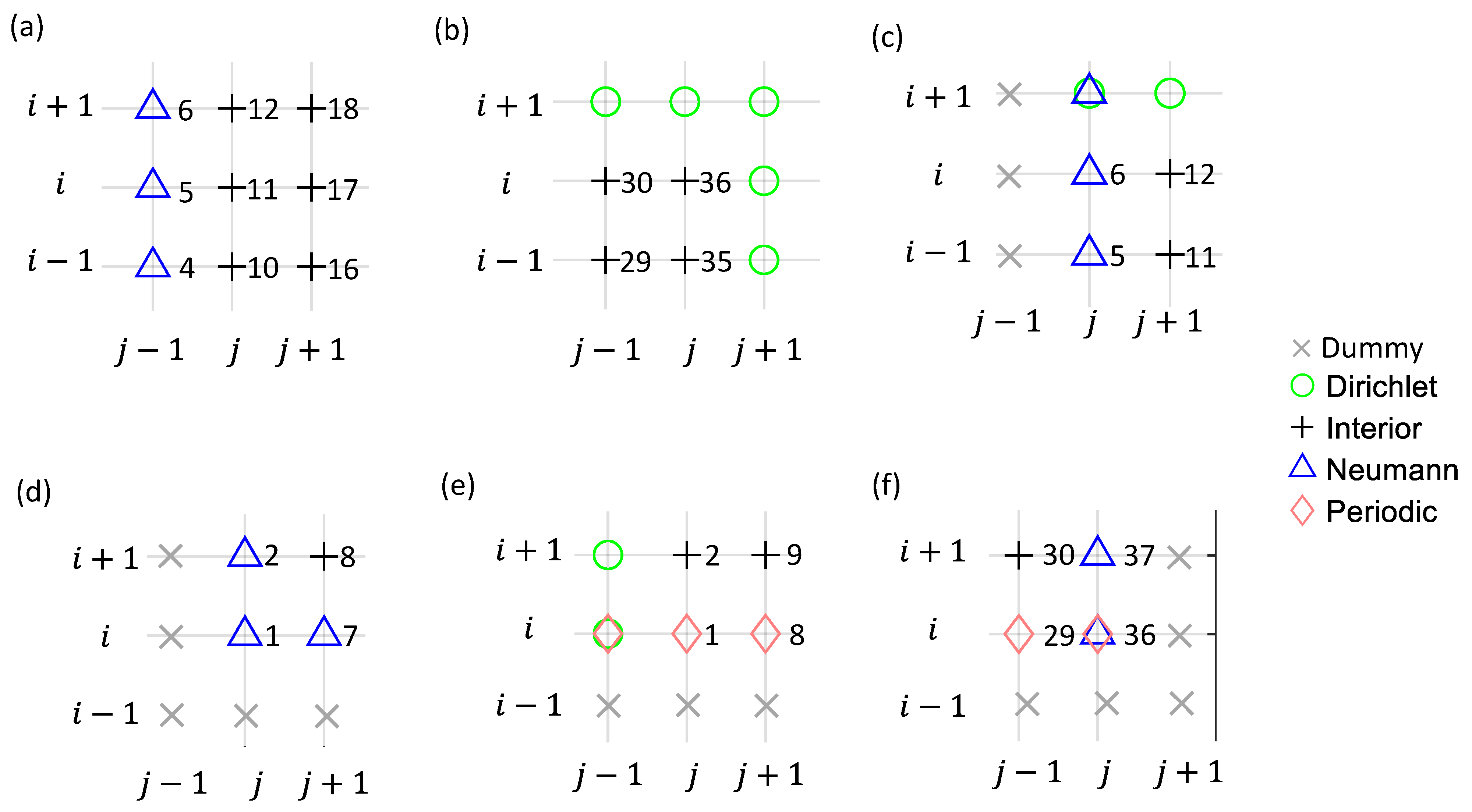
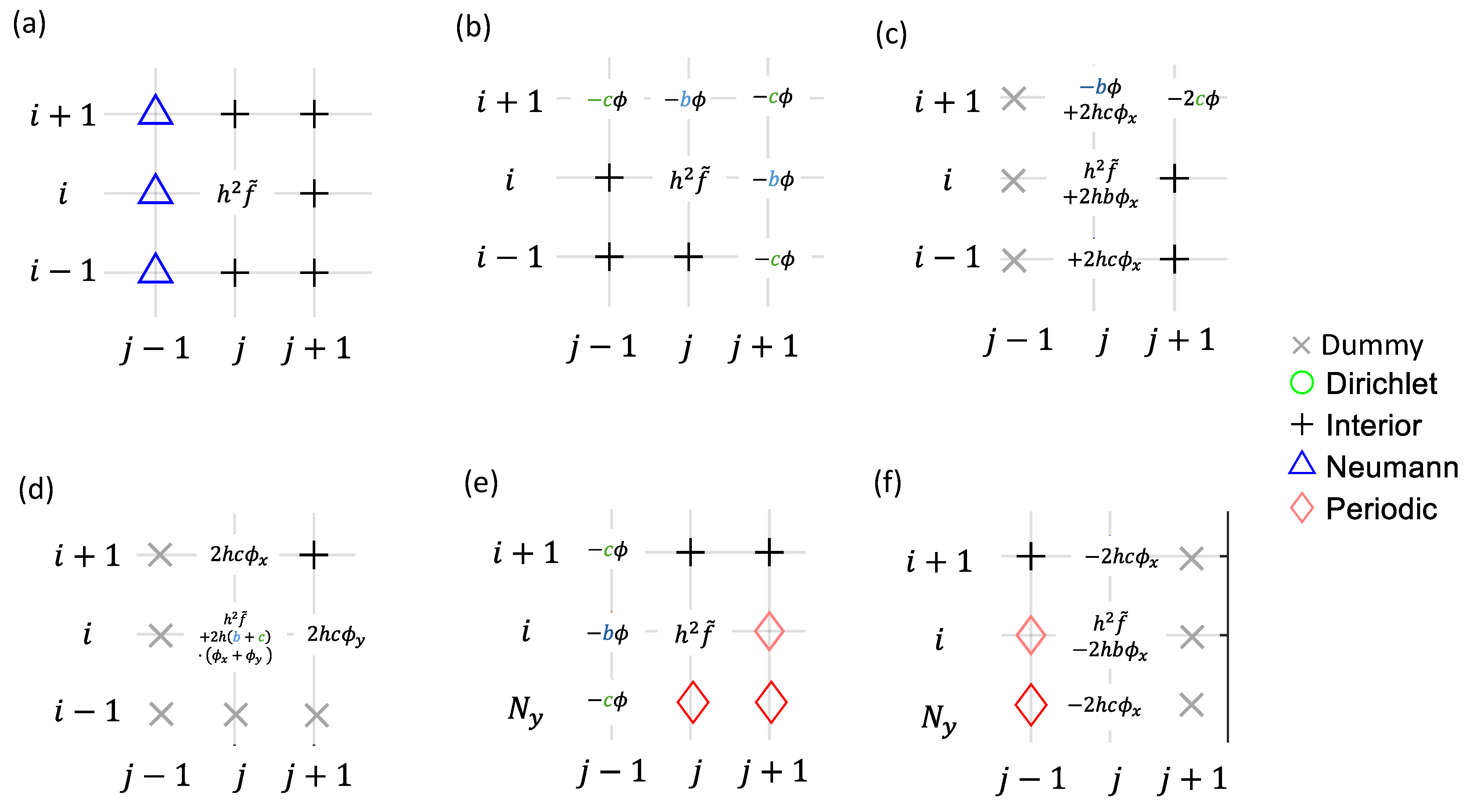
The solutions, $\varphi$, are assumed zeros on grid nodes except for the Dirichlet nodes. Next, for the Dummy nodes outside the Periodic boundaries (e.g., the S and N Dummy nodes in Figure 2b), the nodal values are obtained by copying the Periodic conditions from the opposite side of the domain. Since the solutions are assumed to be zero, this step effectively extends the Dirichlet conditions in the periodic directions. The gradient conditions are copied in the same way if Neumann nodes exist.

(ii)

For the Dummy nodes outside the Neumann boundaries (e.g., W- and S-boundaries in Figure 2a and E-boundary in Figure 2b), the nodal values are obtained by extrapolation using a 2nd-order scheme. Since the solutions are zero before this step, this step effectively assigns the gradient source terms to the Dummy nodes.

(iii)

Consider the extended grid that includes the Dummy nodes and reset boundary conditions such that fringe nodes of the domain are all Dirichlet. These new Dirichlet nodes have nodal values that are equivalent to the effects of Neumann and Periodic BCs.

(iv)

Add the Dirichlet conditions to the RHS source term, $\tilde{f}$, for each solution node. For this step, the routine may first check if the Dirichlet nodes are SW, W, NW, S, N, ES, E, or NE to any solution node, and then the Dirichlet condition is added to the solution node.

By ordering the solution nodes using linear indexing of Equation (4), the results of 2D FD discretization can be written as

$$\mathrm{A}\mathsf{\Phi }=\mathbf{F}$$

(11)

where $\mathsf{\Phi }$ and $\mathbf{F}$ are the solution and source vectors in Equation (5) (2D version), and $\mathrm{A}$ is the square solution matrix formed by the $n_x$ blocks of square matrices of order $n_y$. Using the block matrices for representation, Equation (11) becomes, i.e.,

$$\left[\begin{array}{cccccc}{A}_1& {g_{W}A}_2& & & & {p_{W}A}_2\\ A_2& A_1& A_2& & & \\ & & \ddots & & & \\ & & A_2& A_1& A_2& \\ & & & A_2& A_1& A_2\\ p_E{A}_2& & & & g_E{A}_2& A_1\end{array}\right] \left[\begin{array}{c}\begin{array}{c}{\mathit{\varphi }}_1\\ {\mathit{\varphi }}_2\\ ⋮\end{array}\\ \begin{array}{c}{\mathit{\varphi }}_{\left(n_x-2\right)}\\ {\mathit{\varphi }}_{\left(n_x-1\right)}\\ {\mathit{\varphi }}_{n_x}\end{array}\end{array}\right]=\left[\begin{array}{c}\begin{array}{c}{\tilde{\mathit{f}}}_1\\ {\tilde{\mathit{f}}}_2\\ ⋮\end{array}\\ \begin{array}{c}{\tilde{\mathit{f}}}_{\left(n_x-2\right)}\\ {\tilde{\mathit{f}}}_{\left(n_x-1\right)}\\ {\tilde{\mathit{f}}}_{n_x}\end{array}\end{array}\right]$$

(12)

Here $n_x$ and $n_y$ are the numbers of solution nodes along the x- and y-directions of a rectangular domain; $g_W$, $g_E$, $p_W,$ and $p_E$ are constants depending on BCs of West (W) and North (N) boundaries. The values of these quantities are summarized in Table 2. By summarizing the patterns of the LHS stencil weights for various boundary conditions, e.g., Examples 1 to 3 and Figure 4, the block matrices can be written as follows:

$$A_1={\left[\begin{array}{cccccc}a& g_{S}b& & & & p_{S}b\\ b& a& b& & & \\ & & \ddots & & & \\ & & b& a& b& \\ & & & b& a& b\\ p_{N}b& & & & g_{N}b& a\end{array}\right]}_{n_y\times n_y}$$

(13a)

$$A_2={\left[\begin{array}{cc}\begin{array}{ccc}b& g_{S}c& \\ c& b& c\\ & & \ddots \end{array}& \begin{array}{ccc}\hspace{1em}& \hspace{1em}& p_{S}c\\ & & \\ & & \end{array}\\ \begin{array}{ccc}& & c\\ & & \\ p_{N}c& \hspace{1em}& \hspace{1em}\end{array}& \begin{array}{ccc}b& c& \\ c& b& c\\ & g_{N}c& b\end{array}\end{array}\right]}_{n_y\times n_y}$$

(13b)

Here $g_S$, $g_N$, $p_{S,}$ and $p_N$ are constants depending on BCs of South (S) and North (N) boundaries and are summarized in Table 2. Note that the constants $g$’s and $p$’s are used to discern if the boundary conditions are Neumann or Periodic, respectively, while the subscripts are used to denote which boundary it applies to.

3.2. 2D Modal Decomposition Technique for Solution

This section reviews the background of the matrix decomposition method [10] for solving Equation (12) and generalizes it for 4th-order stencil and various boundary conditions. This review is necessary for continuing the dimensional reduction in the 3D implementation shown in Section 4.2. The technique mainly utilizes modal decomposition of the block matrices. Since the block matrices $A_1$ and $A_2$ can be proved to have the same eigenvectors [27], $Q$, the following modal decomposition can be applied, i.e.,

$$Q^{-1}{A}_{1}Q={\mathrm{\Lambda }}_1$$

(14a)

$$Q^{-1}{A}_{2}Q={\mathrm{\Lambda }}_2$$

(14b)

Here, $Q^{-1}$ denotes the inverse of the eigenvector matrix. If $A_1$ and $A_2$ are symmetric, which applies to the Dirichlet and Periodic conditions (along the y-direction), the eigenvectors are orthogonal, i.e., ${Q^{\mathrm{T}}=Q}^{-1}$. ${\mathrm{\Lambda }}_1$ and ${\mathrm{\Lambda }}_2$ are the diagonal matrices containing the eigenvalues ${\lambda }_{\mathrm{i}}$ and ${\mu }_{\mathrm{i}}$, i.e.,

$${\mathrm{\Lambda }}_1=\mathrm{d}\mathrm{i}\mathrm{a}\mathrm{g}({\mathrm{\lambda }}_1, {\mathrm{\lambda }}_2, \dots ,{\mathrm{\lambda }}_{n_y})$$

(15a)

$${\mathrm{\Lambda }}_2=\mathrm{d}\mathrm{i}\mathrm{a}\mathrm{g}({\mu }_1, {\mu }_2, \dots ,{\mu }_{n_y})$$

(15b)

By pre-multiplying each of the $i$-th rows of Equation (12) by $Q^{-1}$, noting the transformed source term using the overbar, i.e., ${\overline{\tilde{\mathit{f}}}}_j=Q^{-1}{\tilde{\mathit{f}}}_j$, and utilizing the orthogonality of the eigenvectors, ${\mathit{\varphi }}_j=Q{\overline{\mathit{\varphi }}}_j$, for $j=1,2,\dots ,n_x$, Equation (12) becomes

$$\left[\begin{array}{cc}\begin{array}{ccc}{\mathrm{\Lambda }}_1& {g_W\mathrm{\Lambda }}_2& \\ {\mathrm{\Lambda }}_2& {\mathrm{\Lambda }}_1& {\mathrm{\Lambda }}_2\\ \hspace{1em}& \hspace{1em}& \ddots \end{array}& \begin{array}{ccc}\hspace{1em}& \hspace{1em}& {p_W\mathrm{\Lambda }}_2\\ \hspace{1em}& \hspace{1em}& \hspace{1em}\\ \hspace{1em}& \hspace{1em}& \hspace{1em}\end{array}\\ \begin{array}{ccc}\hspace{1em}& \hspace{1em}& {\mathrm{\Lambda }}_2\\ \hspace{1em}& \hspace{1em}& \hspace{1em}\\ p_E{\mathrm{\Lambda }}_2& \hspace{1em}& \hspace{1em}\end{array}& \begin{array}{ccc}{\mathrm{\Lambda }}_1& {\mathrm{\Lambda }}_2& \hspace{1em}\\ {\mathrm{\Lambda }}_2& {\mathrm{\Lambda }}_1& {\mathrm{\Lambda }}_2\\ \hspace{1em}& g_E{\mathrm{\Lambda }}_2& {\mathrm{\Lambda }}_1\end{array}\end{array}\right] \left[\begin{array}{c}\begin{array}{c}{\overline{\mathit{\varphi }}}_1\\ {\overline{\mathit{\varphi }}}_2\\ ⋮\end{array}\\ \begin{array}{c}{\overline{\mathit{\varphi }}}_{\left(n_x-2\right)}\\ {\overline{\mathit{\varphi }}}_{\left(n_x-1\right)}\\ {\overline{\mathit{\varphi }}}_{n_x}\end{array}\end{array}\right]=\left[\begin{array}{c}\begin{array}{c}{\overline{\tilde{\mathit{f}}}}_1\\ {\overline{\tilde{\mathit{f}}}}_2\\ ⋮\end{array}\\ \begin{array}{c}{\overline{\tilde{\mathit{f}}}}_{\left(n_x-2\right)}\\ {\overline{\tilde{\mathit{f}}}}_{\left(n_x-1\right)}\\ {\overline{\tilde{\mathit{f}}}}_{n_x}\end{array}\end{array}\right]$$

(16)

Since the eigenvalue matrices are diagonal, the equations associated with each mode in Equation (16) are independent. For the $i$-th mode, it is

$${\left[\begin{array}{ccc}\begin{array}{cc}{\mathrm{\lambda }}_i& g_W{\mu }_i\\ {\mu }_i& {\mathrm{\lambda }}_i\end{array}& \begin{array}{cc}\hspace{1em}& \hspace{1em}\\ {\mu }_i& \hspace{1em}\end{array}& \begin{array}{cc}\hspace{1em}& {p_W\mu }_i\\ \hspace{1em}& \hspace{1em}\end{array}\\ \begin{array}{cc}\hspace{1em}& {\mu }_i\\ \hspace{1em}& \hspace{1em}\end{array}& \begin{array}{cc}{\mathrm{\lambda }}_i& {\mu }_i\\ \hspace{1em}& \ddots \end{array}& \begin{array}{cc}\hspace{1em}& \hspace{1em}\\ \hspace{1em}& \hspace{1em}\end{array}\\ \begin{array}{cc}\hspace{1em}& \hspace{1em}\\ {p_E\mu }_i& \hspace{1em}\end{array}& \begin{array}{cc}\hspace{1em}& {\mu }_i\\ \hspace{1em}& \hspace{1em}\end{array}& \begin{array}{cc}{\mathrm{\lambda }}_i& {\mu }_i\\ {g_E\mu }_i& {\mathrm{\lambda }}_i\end{array}\end{array}\right]}_{n_x\times n_x}\left[\begin{array}{c}\begin{array}{c}{\overline{\varphi }}_{i,1}\\ {\overline{\varphi }}_{i,2}\\ ⋮\end{array}\\ \begin{array}{c}{\overline{\varphi }}_{i,\left(n_x-2\right)}\\ {\overline{\varphi }}_{i,\left(n_x-1\right)}\\ {\overline{\varphi }}_{i,n_x}\end{array}\end{array}\right]=\left[\begin{array}{c}\begin{array}{c}{\overline{\tilde{f}}}_{i,1}\\ {\overline{\tilde{f}}}_{i,2}\\ ⋮\end{array}\\ \begin{array}{c}{\overline{\tilde{f}}}_{i,\left(n_x-2\right)}\\ {\overline{\tilde{f}}}_{i,\left(n_x-1\right)}\\ {\overline{\tilde{f}}}_{i, n_x}\end{array}\end{array}\right]$$

(17a)

Equation (17a) can be rewritten in an abbreviated form, i.e.,

$${\mathrm{\Gamma }}_i{\widehat{\mathit{\varphi }}}_i={\widehat{\tilde{\mathit{f}}}}_i, i=1, 2, \dots ,n_y$$

(17b)

Here ${\mathrm{\Gamma }}_i$ is the tridiagonal square matrix collecting the eigenvalues of the $i$-th mode; ${\widehat{\mathit{\varphi }}}_i$ and ${\widehat{\tilde{\mathit{f}}}}_i$ denote, respectively, the transformed solution and source vectors of the $i$-th mode.

With the modal decomposition technique described in Equations (14)–(17), the solution algorithm is as follows:

• Compute the eigenvector matrix, $Q$, and diagonal matrices of eigenvalues, ${\mathrm{\Lambda }}_1$ and ${\mathrm{\Lambda }}_2$, for matrices $A_1$ and $A_2$, respectively.
• Compute transformed source vectors, i.e., ${\overline{\tilde{\mathit{f}}}}_j=Q^{-1}{\tilde{\mathit{f}}}_j$, for $j=1,2,\dots ,n_x$.
• Collect the transformed source of the $i$-th mode to form the vector: ${\widehat{\tilde{\mathit{f}}}}_i={\left[{\overline{\tilde{f}}}_{i,1},{\overline{\tilde{f}}}_{i,2},\dots ,{\overline{\tilde{f}}}_{i,n_x}\right]}^{\mathrm{T}}$, and form the tridiagonal eigenvalue matrix ${\mathrm{\Gamma }}_i$.
• Solve the transformed solution of the $i$-th mode, ${\widehat{\mathit{\varphi }}}_i={\left[{\overline{\varphi }}_{i,1},{\overline{\varphi }}_{i,2},\dots ,{\overline{\varphi }}_{i,n_x}\right]}^T$, for $i=1,2,\dots ,n_y$, from the system Equation (17).
• Transform back to the solution by ${\mathit{\varphi }}_j=Q{\overline{\mathit{\varphi }}}_j$ for $j=1,2,\dots ,n_x$.

A few things can be observed when using the matrix decomposition method. Firstly, the 2D FD discretization of Poisson’s equation generates a large sparse solution matrix of order $\left(n_x{n}_y\right)\times \left(n_x{n}_y\right)$ (i.e., Equation (12)). Direct matrix inversion of such a large matrix would require large computer memory as well as computational time. In the matrix decomposition method of Equation (17), the solution matrix is reduced to a tridiagonal one of order $n_y\times n_y$, which is equivalent to solving a 1D system along the y-direction. Although the matrix needs to be inverted for $n_y$ modes, the process is independent of each other and therefore faster. Secondly, the eigenvectors, $Q$, and the inversion of the tridiagonal matrix, ${\mathrm{\Gamma }}_i$, can be predetermined and stored for repeated use if the grid does not change its geometry. This is favorable in reducing the computational time by removing the calculation of the eigenvalue problem for each time step in the simulation of the temporal evolution of the problem. To preserve the accuracy intended by the FD discretization, the contributions of all $n_{\mathrm{y}}$ modes are considered in the modal decomposition and reconstruction. The only exception is the rare case where the transformed source vector, i.e., ${\widehat{\tilde{\mathit{f}}}}_i$ in Equation (17b), is observed to be a zero vector, in which case its modal contribution can be neglected.

In the matrix decomposition, the eigenvectors and eigenvalues can be prescribed analytically and, hence, remove the need for calculation. Swarztrauber [12] provides a valuable summary of these formulations for the typical 2nd-order accurate FD stencil and various BCs (on the South and North boundaries). However, as noted by Cohen [27], because the general form of the block matrix can be obtained by a linear combination of basic 2nd-order discretization and an identity matrix, the eigenvectors of the block matrix associated with the 4th-order discretization should be the same as the 2nd-order ones. The eigenvalues, on the other hand, are different in the 4th-order discretization and, therefore, need to be modified from those prescribed in [12]. This work presents the adapted formulations of eigenvectors and eigenvalues in Appendix A for completeness of the proposed method.

4. Matrix Decomposition Method for 3D Poisson’s Equation

4.1. Linear System of the Discretization

By generalizing the results of the 2D FD discretization, the 3D FD discretization of Poisson’s equation results in the following linear system:

$$M\mathsf{\Phi }=\mathbf{F}$$

(18a)

Since the components of the solutions $\mathsf{\Phi }$ and sources $\mathbf{F}$ are ordered as in Equation (5), the square matrix $M$ formed by $n_z$ block matrices $A$ and $T$ can be summarized as follows as the results of the 3D FD discretization, i.e.,

$$M={\left[\begin{array}{cc}\begin{array}{ccc}A& g_{B}T& \\ T& A& T\\ & & \ddots \end{array}& \begin{array}{ccc}\hspace{1em}& \hspace{1em}& p_{B}T\\ & & \\ & & \end{array}\\ \begin{array}{ccc}& & T\\ & & \\ p_{T}T& \hspace{1em}& \hspace{1em}\end{array}& \begin{array}{ccc}A& T& \\ T& A& T\\ & g_{T}T& A\end{array}\end{array}\right]}_{\left(n_z\mathrm{b}\mathrm{l}\mathrm{o}\mathrm{c}\mathrm{k}\mathrm{s}\right)\times \left(n_z\mathrm{b}\mathrm{l}\mathrm{o}\mathrm{c}\mathrm{k}\mathrm{s}\right)}$$

(18b)

Note that the number of blocks, $n_z$, and the coefficients, $g_B$, $p_B$, $g_T,$ and $p_T$ in $M$ will depend on the boundary conditions of the Bottom (B) and Top (T) faces of the domain, i.e., the two ends in the z-direction. These numbers are summarized in Table 2. The block matrices $A$ and $T$ are used to link the nodal values on the k-th xy-plane to its top ((k+1)-th) and bottom ((k−1)-th) neighbor of the xy-planes. The matrices $A$ and $T$ can be further decomposed into square matrices formed by $n_x$ blocks as follows:

$$A={\left[\begin{array}{cc}\begin{array}{ccc}{A}_1& {g_{W}A}_2& \\ A_2& A_1& A_2\\ & & \ddots \end{array}& \begin{array}{ccc}\hspace{1em}& \hspace{1em}& {p_{W}A}_2\\ & & \\ & & \end{array}\\ \begin{array}{ccc}& & A_2\\ & & \\ p_E{A}_2& \hspace{1em}& \hspace{1em}\end{array}& \begin{array}{ccc}{A}_1& A_2& \\ A_2& A_1& A_2\\ & g_E{A}_2& A_1\end{array}\end{array}\right]}_{\left(n_x\mathrm{b}\mathrm{l}\mathrm{o}\mathrm{c}\mathrm{k}\mathrm{s}\right)\times \left(n_x\mathrm{b}\mathrm{l}\mathrm{o}\mathrm{c}\mathrm{k}\mathrm{s}\right)}$$

(18c)

$$T={\left[\begin{array}{cc}\begin{array}{ccc}{T}_1& g_W{T}_2& \\ T_2& T_1& T_2\\ & & \ddots \end{array}& \begin{array}{ccc}\hspace{1em}& \hspace{1em}& p_W{T}_2\\ & & \\ & & \end{array}\\ \begin{array}{ccc}& & T_2\\ & & \\ p_E{T}_2& \hspace{1em}& \hspace{1em}\end{array}& \begin{array}{ccc}{T}_1& T_2& \\ T_2& T_1& T_2\\ & {g_{E}T}_2& T_1\end{array}\end{array}\right]}_{\left(n_x\mathrm{b}\mathrm{l}\mathrm{o}\mathrm{c}\mathrm{k}\mathrm{s}\right)\times \left(n_x\mathrm{b}\mathrm{l}\mathrm{o}\mathrm{c}\mathrm{k}\mathrm{s}\right)}$$

(18d)

Here $A_1$ and $A_2$ are the matrices that link the nodal values on the j-th line to its East ((j+1)-th) and West ((j−1)-th) neighbor lines of the grids in the y-direction on the k-th xy-plane. Note that the matrix $A$ in Equation (18c) has the block matrices $A_1$ and $A_2$ being the same as in Equation (13) used in 2D discretization. Matrices $T_1$ and $T_2$ do similar jobs as for $A_1$ and $A_2$, respectively, for the nodes on the upper ((k+1)-th) and lower ((k−1)-th) xy-planes, i.e.,

$$T_1={\left[\begin{array}{cc}\begin{array}{ccc}b& g_{S}c& \\ c& b& c\\ & & \ddots \end{array}& \begin{array}{ccc}\hspace{1em}& \hspace{1em}& p_{S}c\\ & & \\ & & \end{array}\\ \begin{array}{ccc}& & c\\ & & \\ p_{N}c& \hspace{1em}& \hspace{1em}\end{array}& \begin{array}{ccc}b& c& \\ c& b& c\\ & g_{N}c& b\end{array}\end{array}\right]}_{n_y\times n_y}$$

(18e)

$$T_2={\left[\begin{array}{cc}\begin{array}{ccc}c& g_{S}d& \\ d& c& d\\ & & \ddots \end{array}& \begin{array}{ccc}\hspace{1em}& \hspace{1em}& p_{S}d\\ & & \\ & & \end{array}\\ \begin{array}{ccc}& & d\\ & & \\ p_{N}d& \hspace{1em}& \hspace{1em}\end{array}& \begin{array}{ccc}c& d& \\ d& c& d\\ & p_{N}d& c\end{array}\end{array}\right]}_{n_y\times n_y}$$

(18f)

In $A_1$ (Equation (13a)), the coefficients $a$ and $b$ link the nodal values on the i-th center node to its South ((i−1)-th) and North ((i+1)-th) neighbors on the j-th line of the grids in the y-direction. The coefficients $b$ and $c$ in matrix $A_2$ (Equation (13b)) do the same thing as $a$ and $b$ in $A_1$, respectively, but for the (j+1)- and (j−1)-th lines of the grids in the y-direction. The same rule can be applied to explain the coefficients $b$, $c,$ and $d$ in $T_1$ and $T_2$ for nodes on the upper ((k+1)-th) and lower ((k−1)-th) neighbors of the k-th xy-plane. These values are summarized in Table 2 as well.

To evaluate the source terms ($\mathbf{F}$) induced by various boundary conditions, the equivalent Dirichlet BCs proposed in Section 3.1—generalized directly from the 2D version—are used. This approach avoids the added complexity of implementing a 3D-specific computer routine.

4.2. 3D Modal Decomposition Technique for Solution

This section expands the modal decomposition technique described in Section 3.2 from 2D to 3D. The way Shiferaw and Mittal [19] started the derivation is first followed but ends up with a more general result that could account for various combinations of BCs. Note that the matrix decomposition results presented in [19] can only be applied to the Dirichlet BCs, and the formulations of the associated eigenvalues are presented without explanation. Here it deduces in detail how the 3D problem with various BCs can be reduced to independent 1D tridiagonal systems using this technique for a fast solution.

Since the stencil coefficients are symmetric (Figure 1), the eigenvectors of matrices $A_1$, $A_2$, $T_1,$ and $T_2$ are the same (see argument in [27]) and, hence, can be assumed as $Q$. The eigenvalues, on the other hand, need to be distinguished. For matrices $A_1$ and $A_2$, the corresponding eigenvalues ${\mathrm{\Lambda }}_1$ and ${\mathrm{\Lambda }}_2$ are obtained using Equations (14) and (15). For matrices $T_1$ and $T_2$, the eigenvalues are obtained in a similar way, i.e.,

$$Q^{-1}{T}_{1}Q={\mathrm{\Omega }}_1$$

(19a)

$$Q^{-1}{T}_{2}Q={\mathrm{\Omega }}_2$$

(19b)

where ${\mathrm{\Omega }}_1$ and ${\mathrm{\Omega }}_2$ are the diagonal matrix of order $n_y$ containing the eigenvalues, i.e.,

$${\mathrm{\Omega }}_1=\mathrm{d}\mathrm{i}\mathrm{a}\mathrm{g}\left({\alpha }_1, {\mathrm{\alpha }}_2, \dots ,{\mathrm{\alpha }}_{n_y}\right)$$

(20a)

$${\mathrm{\Omega }}_2=\mathrm{d}\mathrm{i}\mathrm{a}\mathrm{g}\left({\beta }_1, {\beta }_2, \dots ,{\beta }_{n_y}\right)$$

(20b)

Note that if the BCs on South-North boundaries, i.e., the two ends in the y-direction, are Dirichlet-Dirichlet or Periodic-Periodic, the matrices $A_1$, $A_2$, $T_1,$ and T₂ are symmetric, and, hence, the orthogonality of the eigenvectors, i.e., $Q^{\mathrm{T}}=Q^{-1}$, can be applied.

Now let $\tilde{Q}$ be the matrix containing $n_x$ blocks of $Q$ in the diagonal blocks, i.e.,

$$\tilde{Q}={\left[\begin{array}{cc}\begin{array}{ccc}Q& & \\ & Q& \end{array}& \begin{array}{cc}& \\ & \end{array}\\ \begin{array}{ccc}\hspace{1em}& \hspace{1em}& \ddots \\ & & \\ & & \end{array}& \begin{array}{cc}& \\ Q& \\ & Q\end{array}\end{array}\right]}_{\left(n_x \mathrm{b}\mathrm{l}\mathrm{o}\mathrm{c}\mathrm{k}s\right)\times \left(n_x \mathrm{b}\mathrm{l}\mathrm{o}\mathrm{c}\mathrm{k}s\right)}$$

(21)

and the corresponding eigenvalue matrices of the same order follow:

$${\tilde{Q}}^{-1}A\tilde{Q}=\mathrm{\Lambda }=\left[\begin{array}{cc}\begin{array}{ccc}{\mathrm{\Lambda }}_1& g_W{\mathrm{\Lambda }}_2& \\ {\mathrm{\Lambda }}_2& {\mathrm{\Lambda }}_1& {\mathrm{\Lambda }}_2\\ & {\mathrm{\Lambda }}_2& {\mathrm{\Lambda }}_1\end{array}& \begin{array}{ccc}\hspace{1em}& \hspace{1em}& p_W{\mathrm{\Lambda }}_2\\ \hspace{1em}& {\mathrm{\Lambda }}_1& \\ {\mathrm{\Lambda }}_2& & \end{array}\\ \begin{array}{ccc}\hspace{1em}& \hspace{1em}& {\mathrm{\Lambda }}_1\\ & & \\ {p_E\mathrm{\Lambda }}_2& \hspace{1em}& \hspace{1em}\end{array}& \begin{array}{ccc}\ddots & & \\ {\mathrm{\Lambda }}_2& {\mathrm{\Lambda }}_1& {\mathrm{\Lambda }}_2\\ & g_E{\mathrm{\Lambda }}_2& {\mathrm{\Lambda }}_1\end{array}\end{array}\right]$$

(22a)

$${\tilde{Q}}^{-1}T\tilde{Q}=\mathrm{\Omega }=\left[\begin{array}{cc}\begin{array}{ccc}{\mathrm{\Omega }}_1& g_W{\mathrm{\Omega }}_2& \\ {\mathrm{\Omega }}_2& {\mathrm{\Omega }}_1& {\mathrm{\Omega }}_2\\ & {\mathrm{\Omega }}_2& {\mathrm{\Omega }}_1\end{array}& \begin{array}{ccc}& & p_W{\mathrm{\Omega }}_2\\ & {\mathrm{\Lambda }}_1& \\ {\mathrm{\Omega }}_2& & \end{array}\\ \begin{array}{ccc}& & {\mathrm{\Lambda }}_1\\ & & \\ {p_E\mathrm{\Omega }}_2& \hspace{1em}& \hspace{1em}\end{array}& \begin{array}{ccc}\ddots & & \\ {\mathrm{\Omega }}_2& {\mathrm{\Omega }}_1& {\mathrm{\Omega }}_2\\ & g_E{\mathrm{\Omega }}_2& {\mathrm{\Omega }}_1\end{array}\end{array}\right]$$

(22b)

Recall in Equation (7) that ${\mathit{\varphi }}_k$ and ${\tilde{\mathit{f}}}_k$ are used to denote the vectors collecting, respectively, the solutions and sources on nodes of the k-th xy-plane. Then the discretized system, Equation (18a), can be expanded as

$$A {\mathit{\varphi }}_1+g_{B}T {\mathit{\varphi }}_2 +p_{B}T {\mathit{\varphi }}_{n_z} ={\tilde{\mathit{f}}}_1$$

(23a)

$$T {\mathit{\varphi }}_1+ A {\mathit{\varphi }}_2+T {\mathit{\varphi }}_3 ={\tilde{\mathit{f}}}_2$$

(23b)

$$\dots$$

$$T {\mathit{\varphi }}_{\left(n_z-2\right)}+A {\mathit{\varphi }}_{\left(n_z-1\right)}+T {\mathit{\varphi }}_{n_z}={\tilde{\mathit{f}}}_{\left(n_z-1\right)}$$

(23c)

$$p_{T}T {\mathit{\varphi }}_1 +g_{T}T {\mathit{\varphi }}_{\left(n_z-1\right)}+A {\mathit{\varphi }}_{n_z}={\tilde{\mathit{f}}}_{n_z}$$

(23d)

By pre-multiplying the above equations by ${\tilde{Q}}^{-1}$ to obtain the transform, ${\overline{\tilde{\mathit{f}}}}_k={\tilde{Q}}^{-1}{\tilde{\mathit{f}}}_k$, and noting the inverse transform, ${\tilde{\mathit{f}}}_k=\tilde{Q} {\overline{\tilde{\mathit{f}}}}_k$, the above equations become

$$\mathrm{\Lambda } {\overline{\mathit{\varphi }}}_1+g_B\mathrm{\Omega } {\overline{\mathit{\varphi }}}_2 +p_B\mathrm{\Omega } {\overline{\mathit{\varphi }}}_{n_z}={\overline{\tilde{\mathit{f}}}}_1$$

(24a)

$$\mathrm{\Omega } {\overline{\mathit{\varphi }}}_1+ \mathrm{\Lambda } {\overline{\mathit{\varphi }}}_2+\mathrm{\Omega } {\overline{\mathit{\varphi }}}_3 ={\overline{\tilde{\mathit{f}}}}_2$$

(24b)

$$\dots$$

$$\mathrm{\Omega } {\overline{\mathit{\varphi }}}_{\left(n_z-2\right)}+\mathrm{\Lambda } {\overline{\mathit{\varphi }}}_{\left(n_z-1\right)}+\mathrm{\Omega } {\overline{\mathit{\varphi }}}_{n_z}={\overline{\tilde{\mathit{f}}}}_{\left(n_z-1\right)}$$

(24c)

$$p_T\mathrm{\Omega } {\overline{\mathit{\varphi }}}_1 +g_T\mathrm{\Omega } {\overline{\mathit{\varphi }}}_{\left(n_z-1\right)}+\mathrm{\Lambda } {\overline{\mathit{\varphi }}}_{n_z}={\overline{\tilde{\mathit{f}}}}_{n_z}$$

(24d)

By collecting the terms associated with the i-th mode and using the sub-indexing for the solution and source vectors, the above equations become the following system:

$$\left[\begin{array}{ll}\begin{array}{ll} \left[\begin{array}{cc}\begin{array}{cc}{\mathrm{\lambda }}_i& g_W{\mathrm{\mu }}_i\\ {\mathrm{\mu }}_i& {\mathrm{\lambda }}_i\end{array}& \begin{array}{cc}\cdots & p_W{\mathrm{\mu }}_i\\ {\mathrm{\mu }}_i& \end{array}\\ \begin{array}{cc}& \ddots \\ p_E{\mathrm{\mu }}_i& \cdots \end{array}& \begin{array}{cc}& \\ g_E{\mathrm{\mu }}_i& {\mathrm{\lambda }}_i\end{array}\end{array}\right]& g_B\left[\begin{array}{cc}\begin{array}{cc}{\mathrm{\alpha }}_i& g_W{\mathrm{\beta }}_i\\ {\mathrm{\beta }}_i& {\mathrm{\alpha }}_i\end{array}& \begin{array}{cc}\cdots & p_W{\mathrm{\beta }}_i\\ {\mathrm{\beta }}_i& \end{array}\\ \begin{array}{cc}& \ddots \\ p_E{\mathrm{\beta }}_i& \cdots \end{array}& \begin{array}{cc}& \\ g_E{\beta }_i& {\alpha }_i\end{array}\end{array}\right]\\ \left[\begin{array}{cc}\begin{array}{cc}{\mathrm{\alpha }}_i& g_W{\mathrm{\beta }}_i\\ {\mathrm{\beta }}_i& {\mathrm{\alpha }}_i\end{array}& \begin{array}{cc}\cdots & p_W{\mathrm{\beta }}_i\\ {\mathrm{\beta }}_i& \end{array}\\ \begin{array}{cc}& \ddots \\ p_E{\mathrm{\beta }}_i& \cdots \end{array}& \begin{array}{cc}& \\ g_E{\beta }_i& {\alpha }_i\end{array}\end{array}\right]& \left[\begin{array}{cc}\begin{array}{cc}{\mathrm{\lambda }}_i& g_W{\mathrm{\mu }}_i\\ {\mathrm{\mu }}_i& {\mathrm{\lambda }}_i\end{array}& \begin{array}{cc}\cdots & p_W{\mathrm{\mu }}_i\\ {\mathrm{\mu }}_i& \end{array}\\ \begin{array}{cc}& \ddots \\ p_E{\mathrm{\mu }}_i& \cdots \end{array}& \begin{array}{cc}& \\ g_E{\mathrm{\mu }}_i& {\mathrm{\lambda }}_i\end{array}\end{array}\right]\end{array}& \begin{array}{ll}\begin{array}{ll}\begin{array}{ccc}\hspace{1em}& \hspace{1em}& \cdots \\ \hspace{1em}& \hspace{1em}& \cdots \end{array}& \begin{array}{cc}& \\ & \end{array}\\ \begin{array}{ccc}\hspace{1em}& \hspace{1em}& \cdots \\ \hspace{1em}& \hspace{1em}& \cdots \end{array}& \begin{array}{cc}& \\ & \end{array}\end{array}& p_B\left[\begin{array}{cc}\begin{array}{cc}{\mathrm{\alpha }}_i& g_W{\mathrm{\beta }}_i\\ {\mathrm{\beta }}_i& {\mathrm{\alpha }}_i\end{array}& \begin{array}{cc}\cdots & p_W{\mathrm{\beta }}_i\\ {\mathrm{\beta }}_i& \end{array}\\ \begin{array}{cc}& \ddots \\ p_E{\mathrm{\beta }}_i& \cdots \end{array}& \begin{array}{cc}& \\ g_E{\beta }_i& {\alpha }_i\end{array}\end{array}\right]\\ \left[\begin{array}{cc}\begin{array}{cc}{\mathrm{\alpha }}_i& g_W{\mathrm{\beta }}_i\\ {\mathrm{\beta }}_i& {\mathrm{\alpha }}_i\end{array}& \begin{array}{cc}\cdots & p_W{\mathrm{\beta }}_i\\ {\mathrm{\beta }}_i& \end{array}\\ \begin{array}{cc}& \ddots \\ p_E{\mathrm{\beta }}_i& \cdots \end{array}& \begin{array}{cc}& \\ g_E{\beta }_j& {\alpha }_i\end{array}\end{array}\right]& \begin{array}{cc}\begin{array}{cc}& \\ & \end{array}& \begin{array}{ccccc}\hspace{1em}& \hspace{1em}& & ⋮& \\ \hspace{1em}& \hspace{1em}& & ⋮& \end{array}\\ \begin{array}{cc}& \\ & \end{array}& \begin{array}{ccccc}\hspace{1em}& \hspace{1em}& & ⋮& \\ \hspace{1em}& \hspace{1em}& & ⋮& \end{array}\end{array}\end{array}\\ \begin{array}{cc}\begin{array}{ll}\begin{array}{llllll}⋮& ⋮& & & & \end{array}& \begin{array}{cc}& \end{array}\end{array}& \begin{array}{cc}\begin{array}{cc}& \end{array}& \begin{array}{ccc}\hspace{1em}& \ddots & \ddots \end{array}\end{array}\\ p_T\left[\begin{array}{cc}\begin{array}{cc}{\mathrm{\alpha }}_i& g_W{\mathrm{\beta }}_i\\ {\mathrm{\beta }}_i& {\mathrm{\alpha }}_i\end{array}& \begin{array}{cc}\cdots & p_W{\mathrm{\beta }}_i\\ {\mathrm{\beta }}_i& \end{array}\\ \begin{array}{cc}& \ddots \\ p_E{\mathrm{\beta }}_i& \cdots \end{array}& \begin{array}{cc}& \\ g_E{\beta }_i& {\alpha }_i\end{array}\end{array}\right] & \begin{array}{cc}\begin{array}{cc}\hspace{1em}& \cdots \\ \hspace{1em}& \cdots \end{array}& \begin{array}{cc}& \\ & \end{array}\\ \begin{array}{cc}\hspace{1em}& \cdots \\ \hspace{1em}& \cdots \end{array}& \begin{array}{cc}& \\ & \end{array}\end{array}\end{array}& \begin{array}{cc}\begin{array}{cc}\begin{array}{cc}& \end{array}& \begin{array}{ccc}\hspace{1em}& \ddots & \ddots \end{array}\end{array}& \begin{array}{cc}\begin{array}{cc}& \end{array}& \begin{array}{cc}⋮& \end{array}\end{array}\\ g_T\left[\begin{array}{cc}\begin{array}{cc}{\mathrm{\alpha }}_i& g_W{\mathrm{\beta }}_i\\ {\mathrm{\beta }}_i& {\mathrm{\alpha }}_i\end{array}& \begin{array}{cc}\cdots & p_W{\mathrm{\beta }}_i\\ {\mathrm{\beta }}_i& \end{array}\\ \begin{array}{cc}& \ddots \\ p_E{\mathrm{\beta }}_i& \cdots \end{array}& \begin{array}{cc}& \\ g_E{\beta }_i& {\alpha }_i\end{array}\end{array}\right]& \left[\begin{array}{cc}\begin{array}{cc}{\mathrm{\lambda }}_i& g_W{\mathrm{\mu }}_i\\ {\mathrm{\mu }}_i& {\mathrm{\lambda }}_i\end{array}& \begin{array}{cc}\cdots & p_W{\mathrm{\mu }}_i\\ {\mathrm{\mu }}_i& \end{array}\\ \begin{array}{cc}& \ddots \\ p_E{\mathrm{\mu }}_i& \cdots \end{array}& \begin{array}{cc}& \\ g_E{\mathrm{\mu }}_i& {\mathrm{\lambda }}_i\end{array}\end{array}\right]\end{array}\end{array}\right]\left\{\begin{array}{c}\begin{array}{c}\begin{array}{c}\begin{array}{c}{\overline{\varphi }}_{i,1,1}\\ {\overline{\varphi }}_{i,2,1}\end{array}\\ \begin{array}{c}⋮\\ {\overline{\varphi }}_{i,n_x,1}\end{array}\end{array}\\ \begin{array}{c}\begin{array}{c}{\overline{\varphi }}_{i,1,2}\\ {\overline{\varphi }}_{i,2,2}\end{array}\\ \begin{array}{c}⋮\\ {\overline{\varphi }}_{i,n_x,2}\end{array}\end{array}\end{array}\\ \begin{array}{c}⋮\\ \begin{array}{c}\begin{array}{c}{\overline{\varphi }}_{i,1,n_z}\\ {\overline{\varphi }}_{i,2,n_z}\end{array}\\ \begin{array}{c}⋮\\ {\overline{\varphi }}_{i,n_x,n_z}\end{array}\end{array}\end{array}\end{array}\right\}=\left\{\begin{array}{c}\begin{array}{c}\begin{array}{c}\begin{array}{c}{\overline{\tilde{f}}}_{i,1,1}\\ {\overline{\tilde{f}}}_{i,2,1}\end{array}\\ \begin{array}{c}⋮\\ {\overline{\tilde{f}}}_{i,n_x,1}\end{array}\end{array}\\ \begin{array}{c}\begin{array}{c}{\overline{\tilde{f}}}_{i,1,2}\\ {\overline{\tilde{f}}}_{i,2,2}\end{array}\\ \begin{array}{c}⋮\\ {\overline{\tilde{f}}}_{i,n_x,2}\end{array}\end{array}\end{array}\\ \begin{array}{c}⋮\\ \begin{array}{c}\begin{array}{c}{\overline{\tilde{f}}}_{i,1,n_z}\\ {\overline{\tilde{f}}}_{i,2,n_z}\end{array}\\ \begin{array}{c}⋮\\ {\overline{\tilde{f}}}_{i,n_x,n_z}\end{array}\end{array}\end{array}\end{array}\right\}$$

(25)

By comparing the 2D finite difference discretization results in Equations (12) and (13), it can be observed that Equation (25) can be thought of as the finite difference discretization of the 2D plane (i.e., the xz-plane) formed by the remaining two directions reduced from modal transformation. The pattern of the equivalent 2D stencil is like the 4th-order stencil with the nodal coefficients replaced by the eigenvalues $a={\mathrm{\lambda }}_i$, $c={\beta }_i$, and $d=0$. However, this reduction does not lead to a symmetric stencil, since for South-North neighbors the stencil weights are $b_{S/N}={\mu }_i$, but for West-East neighbors the stencil weights are $b_{S/N}={\alpha }_i$. The schematic of the equivalent stencil and the reduced 2D grid are shown in Figure 6. By comparing Equation (25) to Equations (12) and (13), it can be seen that the effects of BCs on W, E, B, and T boundaries are preserved in Equation (25), i.e., the locations of $g_W, { g}_E$, $g_B, g_{T,}$ $p_W$, $p_{E,}$ $p_B,$ and $p_T$ in Equation (25) are the same as those of the 2D discretization.

The equivalent 2D discretization in Equation (25) can be further reduced to a 1D linear system using the matrix decomposition method described in Section 3.2. The solution solved from the 1D system can be transformed back to 2D and 3D fields to complete the solution. Such a procedure is summarized as follows:

(i)

Determine the $n_{\mathrm{y}}\times n_{\mathrm{y}}$ eigenvector matrix, $Q$, associated with the boundary conditions in the y-direction, using the results in the Appendix A.

(ii)

Apply the first transform of the source field to obtain $\overline{\tilde{\mathit{f}}}$. This is done through line-wise operation, i.e., ${\overline{\tilde{\mathit{f}}}}_{j,k}=Q^{-1}{\tilde{\mathit{f}}}_{j,k}$ for $j=1,2,\dots ,n_x$ and $k=1, 2,\dots ,n_z$, where ${\overline{\tilde{\mathit{f}}}}_{j,k}$ and ${\tilde{\mathit{f}}}_{j,k}$ are the $n_{\mathrm{y}}\times 1$ vectors in the format of Equation (6) that are used to store nodal values along the y-direction. Permute the first dimension of $\overline{\tilde{\mathit{f}}}$ to the third so that ${\overline{\tilde{f}}}_{i,j,k}$ now becomes ${\overline{\tilde{f}}}_{j,k,i}$.

(iii)

Given an i-th mode, ${\overline{\tilde{\mathit{f}}}}_i$ is now the $\left(n_{\mathrm{x}}{n}_z\right)\times 1$ vector on the RHS of Equation (25). To solve the LHS $\left(n_{\mathrm{x}}{n}_z\right)\times 1$ vector of the transformed solution, ${\overline{\mathit{\varphi }}}_i$, in Equation (25), apply the 2D modal decomposition technique in Section 3.2 based on the equivalent 2D (non-symmetric) compact stencil shown in Figure 6 and the BCs on the xz-planes. Repeat this step for all of the i-th modes ($i=1, 2,\dots ,n_y$) to complete the solution. Once done, reversely permute ${\overline{\varphi }}_{j,k,i}$ to restore its original indexing, ${\overline{\varphi }}_{i,j,k}$ for $\overline{\mathit{\varphi }}$.

(iv)

Conduct an inverse transform to obtain the solution using the line-wise operations similar to step (ii), i.e., ${\mathit{\varphi }}_{j,k}=Q{\overline{\mathit{\varphi }}}_{j,k}$ for $j=1,2,\dots ,n_x$ and $k=1, 2,\dots ,n_z$.

5. Numerical Examples

5.1. General Background

The results of the numerical implementations of the 3D matrix decomposition scheme are presented in this section. To show the ability of the proposed method to account for various boundary conditions (BCs), an example of the BC combinations is shown in Figure 7. The combination of BCs is named in sequence for the six boundary faces: Bottom (B), West (W), South (S), East (E), North (N), and Top (T). Hence, the BCs in Figure 7 are named PDNDDP, where D, N, and P stand for Dirichlet, Neumann, and Periodic BCs, respectively. In the next sections, validations of the proposed method are given for solving the point source field (Section 5.2) and the sinusoidal source fields (Section 5.3) in various combinations of the BCs.

The proposed method is flexible to the stencil weights, as long as it is compact and symmetric. Hence, the order convergence rate can be examined in the validation sections for various 3D stencil weights shown in Table 1. The typical 2nd-order accurate stencil weights and the two 4th-order stencils are applied to obtain numerical solutions. Note that the 4th-order stencil-2 is a common 4th-order stencil seen in [19,25], while the 4th-order stencil-1 is extracted from [19] using the assumption of the uniform grid in each direction. The orders of accuracy are examined by refining mesh grid spacing in a doubly manner, i.e.,

$$h=L_x/2^{k+1}, k=3, 4, 5, 6, 7$$

(26)

where $L_x$ is the length of the domain in the x-direction. The errors of numerical simulations are defined as the absolute deviation from the exact solution, ${\varphi }_{\mathrm{e}\mathrm{x}\mathrm{a}\mathrm{c}\mathrm{t}}\left(\mathbf{x}\right),$ at coordinate $\mathbf{x}=\left(x,y,z\right)$, i.e.,

$$\mathrm{Spatial} \mathrm{error}: \mathrm{\epsilon }\left(\mathbf{x}\right)=\left|{\varphi }_{\mathrm{n}\mathrm{u}\mathrm{m}\mathrm{e}\mathrm{r}\mathrm{i}\mathrm{c}\mathrm{a}\mathrm{l}}\left(\mathbf{x}\right)-{\varphi }_{\mathrm{e}\mathrm{x}\mathrm{a}\mathrm{c}\mathrm{t}}\left(\mathbf{x}\right)\right|$$

(27)

where ${\varphi }_{\mathrm{n}\mathrm{u}\mathrm{m}\mathrm{e}\mathrm{r}\mathrm{i}\mathrm{c}\mathrm{a}\mathrm{l}}\left(\mathbf{x}\right)$ denotes the numerical solution using the proposed method. The statistics of the spatial errors, such as the mean (L₂ norm), ${\mathrm{\epsilon }}_{\mathrm{m}\mathrm{e}\mathrm{a}\mathrm{n}}$, 99.9-percentile, ${\mathrm{\epsilon }}_{99.9\mathrm{\%}}$, and the maximum value, ${\mathrm{\epsilon }}_{\mathrm{m}\mathrm{a}\mathrm{x}}$, are presented for indication of the numerical performances, which are defined as:

$$\begin{array}{}\mathrm{(28a)}& \mathrm{Spatial} \mathrm{averaged} \mathrm{error}: {\mathrm{\epsilon }}_{\mathrm{m}\mathrm{e}\mathrm{a}\mathrm{n}}={\left({\displaystyle \frac{1}{L_x{L}_{\mathrm{y}}{L}_z}}\int {\mathrm{\epsilon }}^2\left(\mathbf{x}\right)d\mathbf{x}\right)}^{0.5}\mathrm{(28b)}& 99.9-\mathrm{percentile} \mathrm{error}: {\mathrm{\epsilon }}_{99.9\mathrm{\%}}=99.9-\mathrm{percentile} \mathrm{of} \mathrm{\epsilon }\left(\mathbf{x}\right)\mathrm{(28c)}& \mathrm{Maximum} \mathrm{error}:{\mathrm{\epsilon }}_{\max }=\mathrm{maximum} \mathrm{of} \mathrm{\epsilon }\left(\mathbf{x}\right)\end{array}$$

In Equation (28a), L_x, L_y, and L_z are the side lengths of the 3D rectangular domain along the x-, y-, and z-directions, respectively.

Note that the use of mean error reflects the overall accuracy, but the effects of scarce large errors may be diluted. If only the peak error is examined, the overall performance may not be sensed. Hence, in this paper, the 99.9th-percentile error is also examined.

In Section 5.4, application examples of the proposed method are presented for some 3D vortex-in-cell flow simulations, which include the collision of two co-axial vortex rings, the flow induced by the impulsively a started sphere and a circular cylinder, as well as the boundary layer flow around the floor-mounted cube at low Reynolds numbers, to demonstrate the need of combined BCs in the practical flow simulations, and how the proposed method can be well-suited for this purpose.

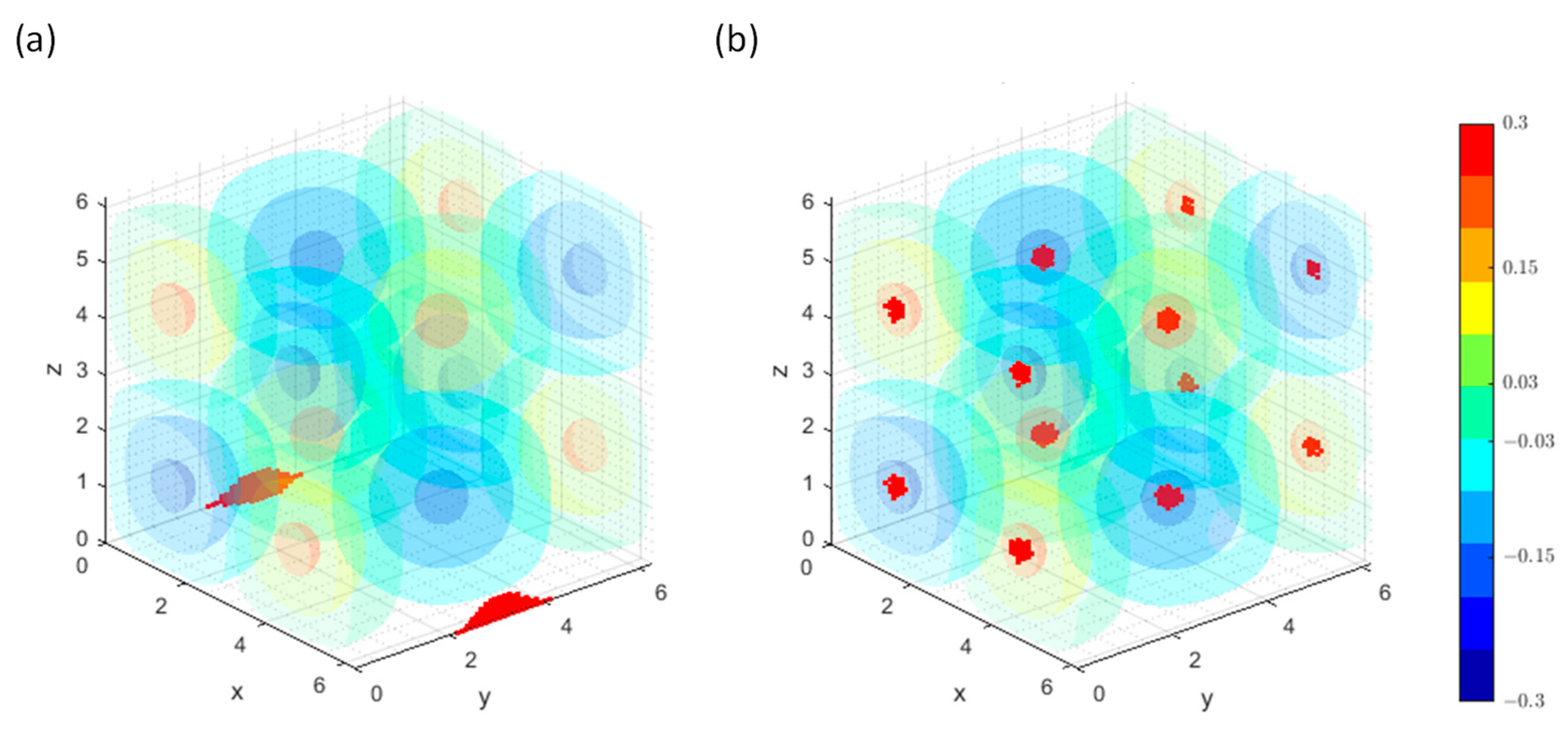
5.2. Validation with the 3D Particle Field

The first example is to use the proposed method to solve Poisson’s equation under the Gaussian particle source, $\zeta$, i.e.,

$$\zeta ={\displaystyle \frac{\mathrm{\Gamma }}{{\left(\sqrt{2\pi } \sigma \right)}^3}}\exp \left(-{\displaystyle \frac{r^2}{2{\sigma }^2}}\right)$$

(29)

Here $\mathrm{\Gamma }$ is the particle strength, $\sigma$ is the smoothing parameter, $r$ is the distance from the particle center, ${\mathbf{x}}_o=x_o{\mathbf{e}}_1+y_o{\mathbf{e}}_2+{\mathrm{z}}_{\mathrm{o}}{\mathbf{e}}_3$, i.e.,

$$r^2={\left(x-x_o\right)}^2+{\left(y-y_o\right)}^2+{\left(z-z_o\right)}^2$$

(30)

Of note, the selection of the point Gaussian source is inspired by the 3D point vorticity distribution in the vortex particle method (e.g., Ploumhans et al. [28]). The resulting Poisson solution to this smoothed point source, $G\left(r\right)$, is used to calculate the particle attribution to the corresponding stream-function field, i.e.,

$${\nabla }^{2}G=-\zeta$$

(31)

Using the Green’s (divergence) theorem in the spherical coordinate, the exact solution to Equation (31) can be obtained, i.e.,

$$G={\displaystyle \frac{1}{\sigma }}{\displaystyle \frac{\sigma }{4\pi r}}\mathrm{erf}\left({\displaystyle \frac{r}{\sqrt{2}\sigma }}\right)$$

(32)

where $\mathrm{e}\mathrm{r}\mathrm{f}\left(s\right)={\int }_0^s\exp \left(-p^2\right)dp$. From Equation (32), the exact Dirichlet BCs can be obtained as well. For the Neumann BCs, the gradient of Equation (32) is also calculated:

$$\nabla G=-{\displaystyle \frac{\mathbf{r}}{4\pi r^3}}\left[\mathrm{erf}\left({\displaystyle \frac{r}{\sqrt{2}\sigma }}\right)-{\displaystyle \frac{r}{\sigma }}\sqrt{{\displaystyle \frac{2}{\pi }}}\exp \left(-{\displaystyle \frac{r^2}{2{\sigma }^2}}\right)\right]$$

(33)

where $\mathbf{r}=\mathbf{x}-{\mathbf{x}}_o$ is the location vector relative to the particle.

For simplicity in the demonstrations, only the effects of one particle are examined. The particle has a unity strength, $\mathrm{\Gamma }=1$, and is located at the origin, i.e., $x_o=y_o=z_o=0$, with $\mathrm{\sigma }=0.2$. A cubic domain with a side length of 2 is chosen (i.e., $L_x=L_y=L_z=2$) and the grid points span within $-L_x/2\le x\le L_x/2,-L_y/2\le y\le L_y/2$, and $-L_z/2\le z\le L_z/2$. For this problem, combinations of Dirichlet and Neumann BCs are studied. The isosurface of the exact solution is shown in Figure 8. As can be seen, the solution has a smooth peak near the origin and gradually decays in the radial direction. The red dots in Figure 8 indicate where the errors of the 4th-order (stencil-1) numerical solutions are larger than the 99.9-percentile value. For the all-Dirichlet BCs (Figure 8a), the largest errors occur near the peak. For the partially Neumann BCs (Figure 8b), the largest errors occur near the center of the Neumann boundary faces. Since the locations of the largest errors are different in Figure 8a,b, the mechanisms causing the error may be different for Dirichlet and Neumann BCs.

More thorough error analyses are shown in Figure 9, which includes the effects of grid spacing, stencil schemes (identified by symbols), and boundary conditions (identified by colors). Also attached in the figure are the auxiliary lines denoting the 4th- and 2nd-order convergence rates. As can be seen, the most accurate results come from the 4th-order schemes in the all-Dirichlet (DDDDDD) conditions. As one of the boundary conditions becomes Neumann, the convergence rate of the 4th-order schemes decreases to 2nd-order. When more boundary conditions become Neumann, the accuracies of both 2nd- and 4th-order schemes decrease. The accuracy reduction rates are less sensitive in the 2nd-order scheme than in the 4th-order schemes when more Neumann boundaries are added.

To see the effectiveness of the 4th-order scheme as compared to the typical 2nd-order scheme for various boundary conditions, the errors of the 4th-order scheme-2 are first divided by the error of the 2nd-order scheme and shown in Figure 10. As can be seen, since the 4th-order scheme works as it claims in the all-Dirichlet BCs, the error ratio decreases in 2nd-order for all-Dirichlet BCs. For other BCs that include Neumann, the error ratio remains constant, manifesting again the reduction of the 4th-order scheme to the 2nd-order. Although the convergence rates decrease, the error ratios of the 4th-order scheme-2 generally remain below unity, except in the extreme case (NNNNND), where the stronger coupling to boundary gradients in the 4th-order stencil dominates the solution. This observation preserves the value of using the 4th-order scheme against the 2nd-order one in Neumann boundaries.

To compare the effectiveness of the two 4th-order schemes in detail, the ratio of the errors obtained from scheme-1 is divided by those of scheme-2. As can be seen in Figure 11, most of the ratios are close to 1, except for all Dirichlet BCs. The reason scheme-1 results in higher errors under all Dirichlet BCs is not yet clear and warrants further investigation. In summary, regarding the effectiveness of the schemes, the 4th-order schemes are mostly better than the 2nd-order scheme, and the 4th-order scheme-2 is slightly better than the 4th-order scheme-1.

The cause of accuracy reduction to the 2nd order of the 4th-order schemes in the presence of the Neumann boundary conditions may be explained by its 2nd-order assumptions in extrapolating the nodal values outside the Neumann boundaries (see examples in Section 3.1). Using this hypothesis, one may retrieve the 4th-order convergence rate if these Neumann boundaries are pushed outward far enough from the region of intense gradients. To examine this point, the errors of different domain lengths in the z-direction, i.e., ${\mathrm{L}}_{\mathrm{z}}=2, 4, 10$, for solutions in boundary condition NDDDDN are plotted in Figure 12. As expected, the 4th-order scheme is almost fully retrieved for ${\mathrm{L}}_{\mathrm{z}}=10$ under this BC, while partially retrieved for ${\mathrm{L}}_{\mathrm{z}}=4$.

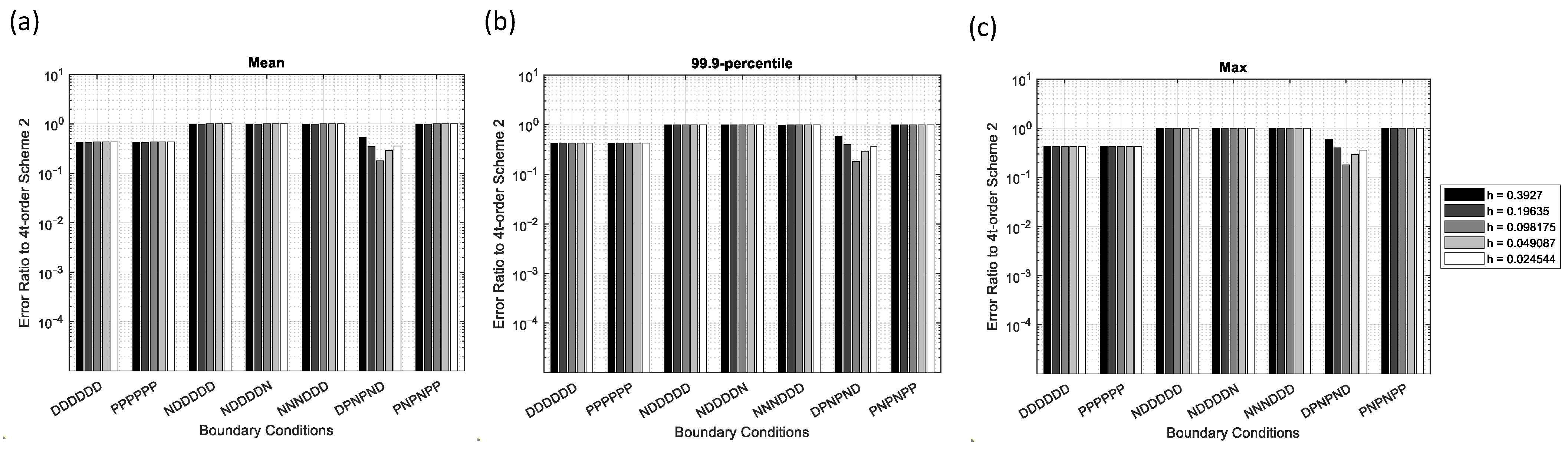
5.3. Validation with the 3D Sinusoidal Field

In this section, the solutions to the sinusoidal source field of the Poisson’s equation are discussed, i.e.,

$$\omega =\sin \left(x\right) \cos \left(y\right) \sin \left(z\right)$$

(34)

$${\nabla }^2\mathsf{\Psi }=-\omega$$

(35)

$$\mathsf{\Psi }=-{\displaystyle \frac{1}{3}}\sin \left(x\right) \cos \left(y\right) \sin \left(z\right)$$

(36)

The fields are periodic, and the domain spans from 0 to $2\pi$ in all three directions, i.e.,$L_x=L_y=L_z=2\pi$ and $0\le x\le L_x,0\le y\le L_y$ and $0\le z\le L_z$. Equation (34) is inspired by Taylor-Green’s formulation for the initial vorticity field (ω), which is commonly used to study turbulence evolution (e.g., [29]). By solving Poisson’s equation (Equation (35)) with Periodic BCs in all directions, the exact stream function solution (ψ) is obtained (Equation (36)). Since this problem is used for validation, combinations of Dirichlet, Neumann, and periodic boundary conditions are assumed for the following discussion. Figure 13 shows the iso-surfaces of the exact solution (Equation (36)) to the Poisson’s equation (Equation (35)), along with the red dots denoting the locations of errors larger than the 99.9-percentile value under BCs NNDNDD (Figure 13a) and PPPPPP (Figure 13b). As can be seen, larger errors are distributed on the edges connecting Neumann boundaries in Figure 13a and near peaks for all Periodic conditions in Figure 13b. The difference in error locations in Figure 13a,b implies different mechanisms in error generation for Neumann and Periodic BCs. The error statistics of Dirichlet and Periodic BCs are shown in Figure 14. It can be seen that the use of the 4th-order and the 2nd-order schemes shows exactly the 4th- and 2nd-order rates of convergence, respectively, under combinations of Dirichlet and Periodic boundary conditions.

When the Neumann BCs are combined with the Dirichlet or Periodic BCs, Figure 15 shows the convergence rates of the 4th-order schemes reduce to 2nd-order, except for the BC DPNPND. The reason that the convergence rate in BC DPNPND is still 4th-order is because of zero y-gradient values on the South and North boundaries. Unlike the point-source field discussed in the previous section, it is not possible to reduce the effects of Neumann conditions by pushing the Neumann boundary outward for this periodic field.

Figure 16 shows the error ratios of the 4th-order scheme-2 to the 2nd-order scheme. Since the 4th-order scheme works as it claims for the Dirichlet and Periodic BCs, the error ratios decrease at the rate of the 2nd-order as the grid spacing reduces. For other BCs that include Neumann, the error ratios shown in Figure 16 are less than or equal to unity for mean errors, manifesting the effectiveness of the 4th-order scheme in the overall solutions. On the other hand, the error ratios can exceed unity for the 99.9th percentile and maximum errors, suggesting that the stronger coupling to boundary gradients in the 4th-order stencil has a greater impact on the solution than in the 2nd-order stencil.

The error ratios of the 4th-order scheme-1 to the 4th-order scheme-2 are shown in Figure 17. As can be seen, scheme-1 is more accurate than scheme-2 for Dirichlet and Periodic conditions. The two schemes have nearly equal accuracy for Dirichlet-Neumann or Neumann-Periodic conditions.

5.4. Discussion on the Applicability of the Efficient Method

In this section, the advantages and disadvantages of the proposed matrix decomposition method are discussed. As mentioned in Section 1, the primary motivation for using this method is its computational efficiency. To demonstrate this, the computational times of Poisson’s solver using both the matrix inversion and matrix decomposition methods are compared for a sinusoidal field (Section 5.2) within a cubic domain ($L_{\mathrm{x}}=L_y=L_z=2\pi$). The comparison is performed for varying numbers of one-sided nodes: $n=10, 20, 30, 40, 50$, and $60$, under a mixed boundary condition (DNPNPD). All calculations are conducted using MATLAB R2022a. For the matrix inversion method, the system matrix $M$ from Equation (18) is explicitly formed, and the solution is computed using MATLAB’s syntax $\mathsf{\Phi }=\mathbf{F}\backslash M$. However, since $M$ is very large—of approximate size $n^3\times n^3$—it must be stored as a sparse matrix (using sparse(M)) to avoid excessive memory usage due to the large number of zero entries. Computational times are measured on a standard desktop computer equipped with an Intel six-core i5-10500 CPU @ 3.10 GHz and 8 GB of RAM.

The resulting computational times are presented in Figure 18, with auxiliary reference lines indicating $O\left(n^6\right)$ and $O\left(n^2\right)$ for comparison. The mean, 99.9th percentile, and maximum errors are identical for both methods, confirming their numerical equivalence. For the matrix inversion technique, the computational time increases approximately with $O\left(n^6\right)$, which corresponds to the total number of entries in the full matrix $M$. In contrast, the matrix decomposition method yields significantly lower computational times, scaling approximately as $O\left(n^2\right)$, which corresponds to the number of nodes along one side of the cubic domain. This confirms that the proposed decomposition method effectively reduces the 3D problem to 1D ones, as discussed in Section 4.2. Consequently, the matrix decomposition method achieves a speed-up factor on the order of $O\left(n^4\right)$.

For the matrix decomposition method shown in Section 4.2 to preserve its efficiency, the general structure of the block matrices in Equation (18) needs to remain. Hence, one may use different spacing in different directions, but the grid needs to be uniform for the current efficient method to work [19,20]. When encountering a problem that requires finer resolution locally, e.g., flow around a solid body, a non-uniform or non-structured grid may be used to reach the overall efficiency of the grid.

If a non-uniform grid is used, one may consider some analytical function to map the non-uniform grid to a uniform one and solve Poisson’s equation in the mapped domain. Such a mapping could lead to spatially varying coefficients multiplied by the second derivatives in the mapped Poisson’s equation and generate additional first derivatives with variable coefficients on the LHS of Equation (1). The discretization of such mapped governing equations cannot be represented by the block matrices presented in the current method and, hence, cannot be solved efficiently using the current scheme. To resolve this issue, typical FD discretization with non-compact stencils and different matrix decomposition schemes [30] may be resorted to. For a non-structured grid, for example, the hierarchically divided square cells used in [31], the FD discretization can be complicated. Developing a method to efficiently solve such a system is even more difficult.

On the other hand, to cope with the discontinuity of source terms, the uniform (or non-uniform) grids may be used with the immersed boundary method (IBM) (e.g., examples in Section 5.5) or the immersed interface method (IIM) (e.g., [32,33,34]). Many new developments have been found in IIMs since they work better to remove the effects due to sharp discontinuity. However, inevitable changes in the local stencil weights near the discontinuity may again lead to different formats of block matrices. In this case, the other format of the matrix decomposition [30] needs to be sought.

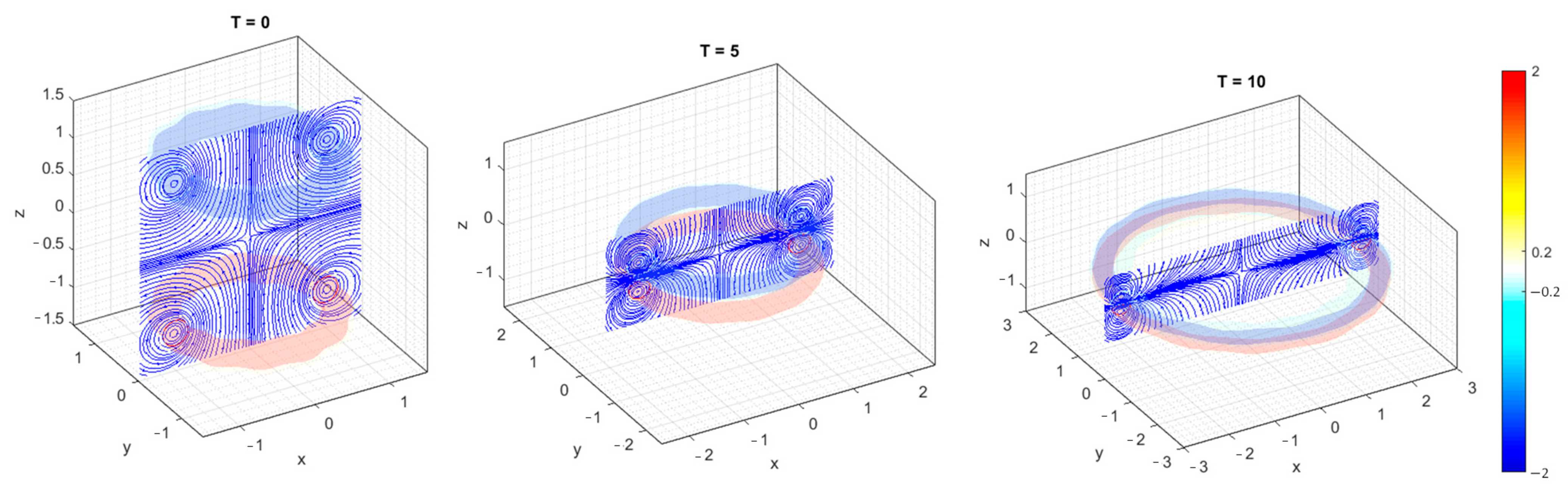
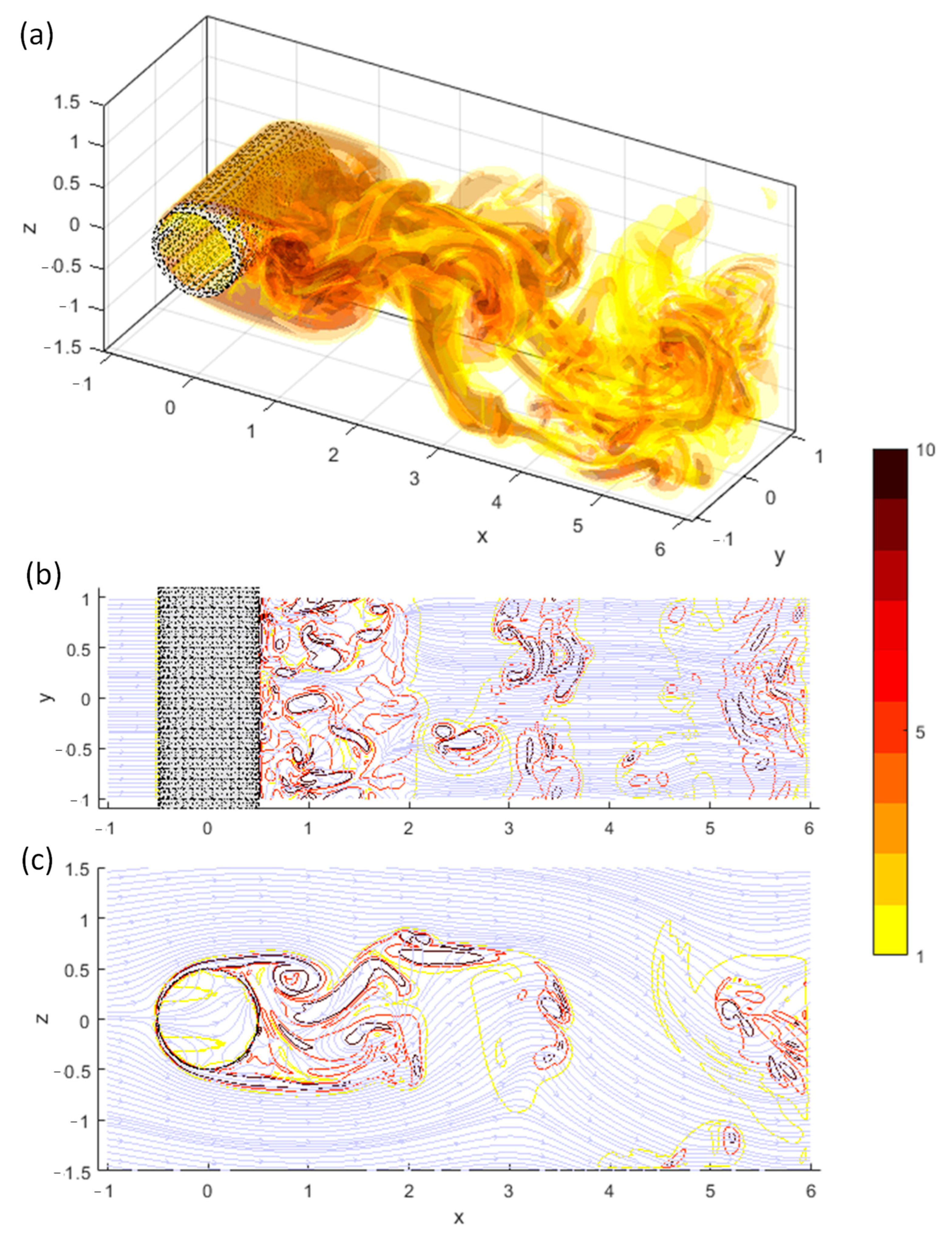
5.5. Applications in the 3D Vortex-In-Cell Flow Simulations

This section presents applications of the proposed Poisson solver with various boundary conditions in 3D vortex-in-cell (VIC) simulations. Detailed VIC algorithms can be found in [35,36,37] and other key references. In the following examples, the stream function vector fields are obtained by solving Poisson’s equation for a given vorticity field using the 4th-order scheme-2 stencil (see Table 1). The velocity field is then computed by differentiating the stream functions, while vorticity advection, stretching, and diffusion are determined based on the vorticity governing equation. To solve Poisson’s equation, Dirichlet conditions for the stream function are derived from the Biot-Savart law and Fast Multipole Methods. Since solving Poisson’s equation for the stream function is only one component of the VIC algorithm, it does not solely determine the accuracy and computational time of the simulations. Therefore, the focus here is not on the convergence rate or the overall computational time. The outline of the flow examples, as well as the corresponding Reynolds number, time increments, grid spacing, and BCs of the Poisson’s solver, are given in

Table 3. Summary of Reynolds numbers (${Re}_{\mathrm{\Gamma }}$ and ${Re}_D$), grid spacings ($h$), time increments ($∆t$), and BCs of the Poisson’s solver used in the flow simulations. The BCs are labeled in the sequence of B-W-S-E-N-T boundaries of the rectangular domain, and D, N, and P are abbreviations of Dirichlet, Neumann, and Periodic conditions, respectively. For vortex ring simulation, ${Re}_{\mathrm{\Gamma }}\equiv \mathrm{\Gamma }/\nu$. For simulations of flow passing bluff bodies. ${Re}_D=u_{\infty }D/\nu$.

Example Flow	$\mathbf{Reynolds} \mathbf{Number}, \mathit{R}\mathit{e}$	$\mathbf{Grid} \mathbf{Spacing}, \mathit{h}$	$\mathbf{Time} \mathbf{Increment}, ∆\mathit{t}$	BCs
Heads-on collision of two vortex rings	${Re}_{\mathsf{\Gamma }}=1000$	$h/R=0.002$	$∆t \mathsf{\Gamma }/R^2=0.01$	DDDDDD
Impulsively started sphere	${Re}_D=500$	$h/D=0.0179$	$∆t u_{\infty }/D=0.01$	DDDDDD
Impulsively started circular cylinder	${Re}_D=1000$	$h/D=0.012$	$∆t u_{\infty }/D=0.01$	DDPDPD
Boundary layer flow passing a cube	${Re}_D=300$	$h/D=0.032$	$∆t u_{\infty }/D=0.02$	DDNDND

.

The first example in Figure 19 presents the evolution of the head-on collision of the coaxial vortex rings. The two vortex rings are initialized at $\mathrm{z}=\pm 1$ with an initial radius of the ring, $R=1$, a vortex tube radius, $\mathrm{\sigma }=0.1$, and an initial circulation of the vortex tubes, $\mathrm{\Gamma }=\pm 1$. The Reynolds number based on the circulation is ${Re}_{\mathrm{\Gamma }}=\mathrm{\Gamma }/\nu =1000$, and $\nu$ is the kinematic viscosity. For this problem, the grid spacing, $h/R=0.01$, and time increments, $∆t \mathrm{\Gamma }/R^2=0.01$, are selected in the simulations, which are similar to the simulations of [38]. The initial vorticity distribution on the cross-sections normal to the vortex tube follows the Gaussian profile. Dirichlet BCs of stream functions on all the boundaries are implemented. As the two vortex rings collide, the flow fields expand the radius of the rings (Figure 19). The stretching effects enhance the vorticity inside the core at the initial stage of the collision. The effects of the diffusion then catch on once the vortex tubes become thin.

The second example, shown in Figure 20, illustrates the flow around an impulsively started sphere, at Reynolds number ${\mathrm{R}\mathrm{e}}_{\mathrm{D}}=u_{\infty }D/\nu =500$, where $u_{\infty }$ is the free stream velocity magnitude and $D$ is the diameter of the sphere. For this problem, the grid spacing, $h/D=0.0179$, and time increments, $∆t u_{\infty }/D=0.01$, are selected in the simulations, which are similar to the simulations of [36]. The effects of the solid body are accounted for using Brinkman’s penalization method for immersed bodies (e.g., [37]). This approach allows the proposed method to incorporate inner boundary effects (e.g., [39]) without modification. This process imposes a strong vorticity layer on the sphere’s surface, which then diffuses into the surrounding field and is advected downstream, generating the separated flow. Dirichlet BCs of stream functions are applied to all domain boundaries. With the sine-wave perturbation of the free-stream velocity (in the z-direction) during $3\le T\le 4$, the wake structure is revealed by the instantaneous vorticity and velocity fields at normalized time $T=u_{\infty }t/D=20.$

The third example extends the second one by expanding the bluff body to infinity in the y-direction. Figure 21 shows the example of the flow induced by an impulsively started circular cylinder at Reynolds number ${\mathrm{R}\mathrm{e}}_{\mathrm{D}}=u_{\infty }D/\nu =1000$ at normalized time $T=u_{\infty }t/D=12.8$. For this problem, the grid spacing, $h/D=0.012$, and time increments, $∆t u_{\infty }/D=0.01$, are selected in the simulations, which are similar to the simulations of [36]. Like the previous example, sine-wave perturbation of the free-stream velocity (in the z-direction) during $3\le T\le 4$ triggers the vortex shedding. In this simulation, the Periodic BCs of stream functions are applied in the y-direction, i.e., the South and North boundaries. For the rest of the boundaries, the Dirichlet BCs are applied. Note that the Dirichlet conditions need to be evaluated by finite periodic shifts of the Dirichlet nodes to account for periodicity in the y-direction (see [35]).

The final example presents a boundary layer flow over a surface-mounted cube (Figure 22) at a Reynolds number of ${Re}_D=u_{\infty }D/\nu =300$, where $u_{\infty }$ denotes the free-stream velocity unaffected by the boundary layer and $D$ is the cube width. For this case, the grid spacing $h/D=0.032$ and time step $∆t u_{\infty }/D=0.02$ are used, representing a slightly coarser spatial and temporal resolution compared to the simulations in [36]. Since the flow is not intended to be periodic in the y-direction, the zero Neumann BCs of stream functions are used in the South and North boundaries (lower and upper boundaries in the y-direction). All the other boundaries are of Dirichlet conditions. Note that to impose the no-through flow conditions on the floor, mirrored image vorticity below the bottom boundary must be imposed first (see [35]). Then, the effects of the vorticity flux of the floor can be imposed using the panel method (e.g., [28]).

6. Conclusions

This paper presents an efficient matrix decomposition method for solving the finite-difference (FD) discretized 3D Poisson’s equation using symmetric 27-point, 4th-order accurate stencils. Key contributions include:

(i)

Extension to various boundary conditions (BCs): The method generalizes previous approaches to effectively handle Dirichlet, Neumann, and Periodic BCs.

(ii)

Efficient source term computation: The use of equivalent Dirichlet nodes simplifies implementation and improves accuracy when computing source terms for Dirichlet, Neumann, and Periodic BCs.

(iii)

Generalized eigenvalue formulation: The method refines existing eigenvalue formulas to better handle the general 4th-order stencil weights.

(iv)

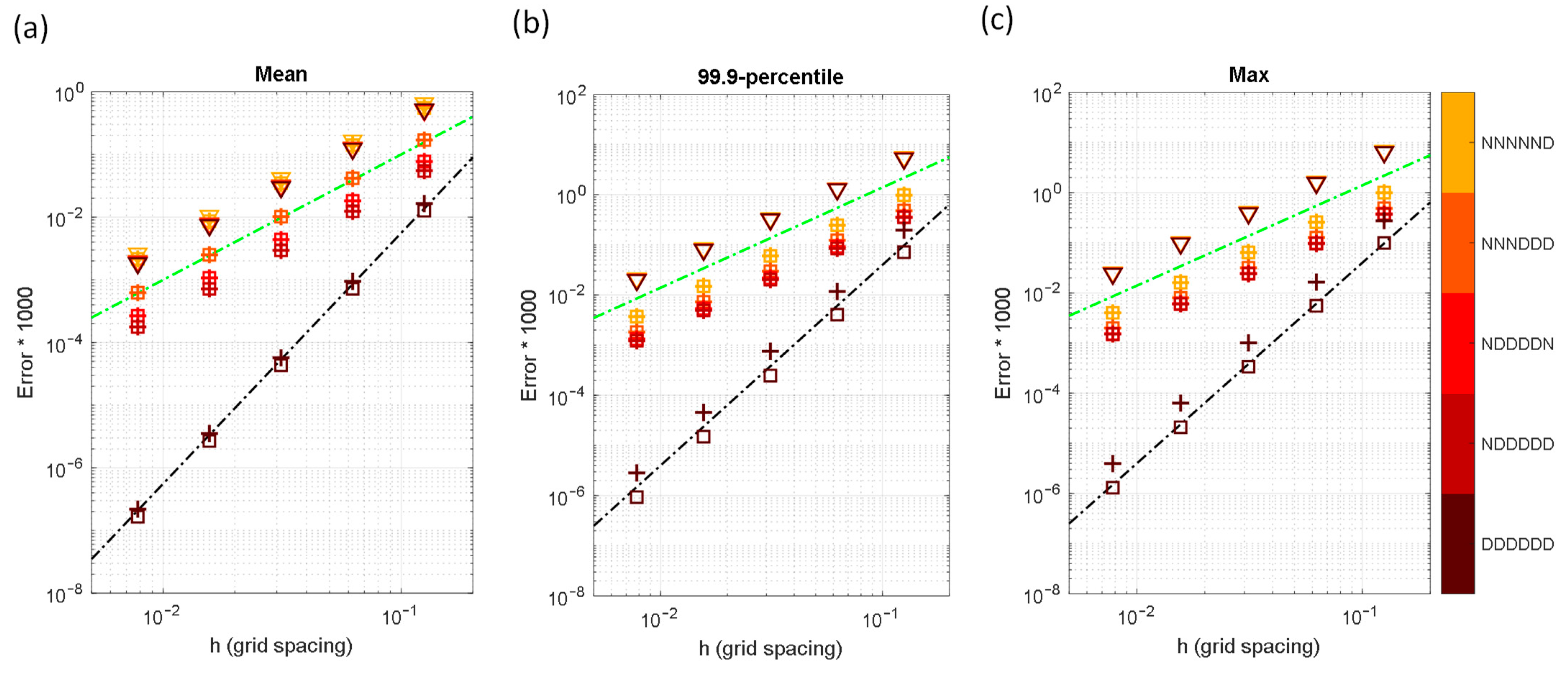
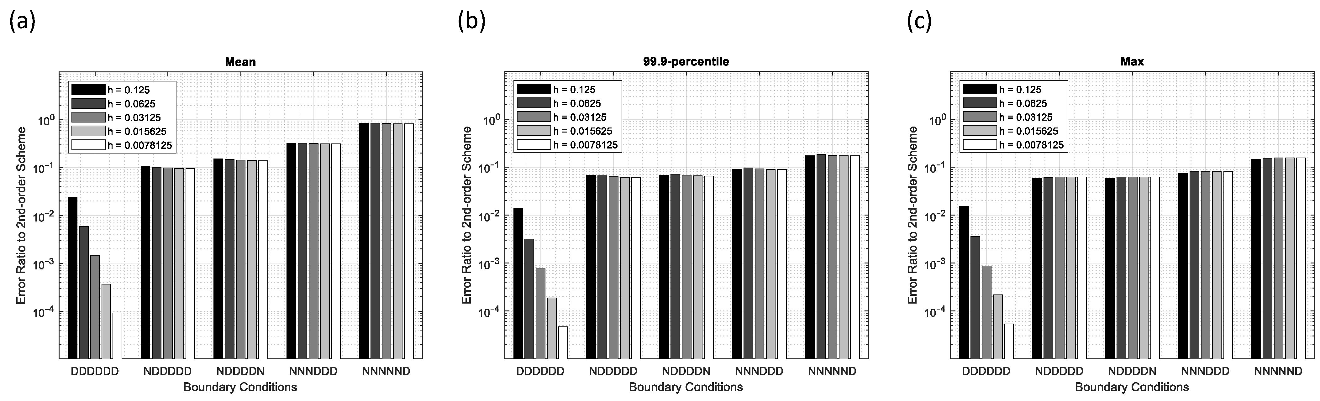
Validation of accuracy: The solver is tested using Gaussian and sinusoidal sources. It achieves 4th-order convergence for Dirichlet and Periodic boundaries. When Neumann boundaries are involved, convergence drops to 2nd-order due to 2nd-order extrapolation but still yields lower mean errors than traditional 2nd-order schemes. More accurate extrapolation methods may be applied in the future to reduce the error for Neumann BCs.

(v)

Application in flow simulation: The method is successfully applied to vortex-in-cell (VIC) simulations. While it primarily manages outer boundaries, it can be used with the immersed boundary method to handle internal solid objects. Neumann and Periodic boundaries also help reduce domain size and improve efficiency. Immersed interface methods may be considered in the future to better handle sharp discontinuity.

References

- Zhong, Y.; Shirinzadeh, B.; Alici, G.; Smith, J. Deformable object simulation with Poisson equation. In Proceedings of the IEEE, International Conference on Mechatronics & Automation, Niagara Falls, ON, Canada, 29 July–1 August 2005; pp. 187–192. [Google Scholar]
- Nagel, J.R. Numerical solutions to Poisson equations using the finite-difference method. IEEE Antennas Propag. Mag. 2014, 56, 209–224. [Google Scholar] [CrossRef]
- Radhakrishnan, A.; Xu, M.; Shahane, S.; Vanka, S.P. A non-nested multilevel method for meshless solution of the Poisson equation in heat transfer and fluid flow. arXiv 2021, arXiv:2104.13758. [Google Scholar] [CrossRef]
- Versteeg, H.; Malalasekera, W. Introduction to Computational Fluid Dynamics: The Finite Volume Method, 2nd ed.; Pearson: London, UK, 2007. [Google Scholar]
- Smith, G.D. Numerical Solutions of Partial Differential Equations: Finite Difference Methods; Oxford University Press: New York, NY, USA, 1985. [Google Scholar]
- Wang, Y.; Zhang, J. Sixth order compact scheme combined with multigrid method and extrapolation technique for 2D Poisson equation. J. Comput. Phys. 2009, 228, 137–146. [Google Scholar] [CrossRef]
- Ge, Y. Multigrid method and fourth-order compact difference discretization scheme with unequal meshsizes for 3D Poisson equation. J. Comput. Phys. 2010, 229, 6381–6391. [Google Scholar] [CrossRef]
- Hockney, R.W. A fast direct solution of Poisson equation using Fourier analysis. JACM 1965, 12, 95–113. [Google Scholar] [CrossRef]
- Buneman, O. A Compact Non-Iterative Poisson Solver; Rep. SUIPR-294; Institute for Plasma Research, Stanford University: Stanford, CA, USA, 1969. [Google Scholar]
- Buzbee, B.L.; Golub, G.H.; Nielson, C.W. On direct methods for solving Poisson’s equations. SIAM J. Numer. Anal. 1970, 7, 627–655. [Google Scholar] [CrossRef]
- Sweet, R.A. A Generalized Cyclic Reduction Algorithm. SIAM J. Numer. Anal. 1974, 11, 506–520. [Google Scholar] [CrossRef]
- Swarztrauber, P.N. The methods of cyclic reduction, Fourier analysis and the FACR algorithm for the discrete solution of Poisson’s equation on a rectangle. SIAM Rev. 1977, 19, 490–501. [Google Scholar] [CrossRef]
- Cooley, J.W.; Lewis, P.A.W.; Welch, P.D. The fast Fourier transform algorithm: Programming considerations in the calculation of sine, cosine and Laplace transforms. J. Sound Vib. 1970, 12, 315–337. [Google Scholar] [CrossRef]
- Swarztrauber, P.N. Symmetric FFTs. Math. Comput. 1986, 47, 323–346. [Google Scholar] [CrossRef]
- Schumann, U.; Sweet, R.A. A direct method for the solution of Poisson’s equation with Neumann boundary conditions on a staggered grid of arbitrary size. J. Comput. Phys. 1976, 20, 171–182. [Google Scholar] [CrossRef]
- Schumann, U.; Sweet, R.A. Fast Fourier transforms for direct solution of Poisson’s equation with staggered boundary conditions. J. Comput. Phys. 1988, 20, 123–137. [Google Scholar] [CrossRef]
- Sweet, R.A. Direct methods for the solution of Poisson’s equation on a staggered grid. J. Comput. Phys. 1973, 12, 422–428. [Google Scholar] [CrossRef]
- Wilhelmson, R.B.; Ericksen, J.H. Direct Solutions for Poisson’s equation in three dimensions. J. Comput. Phys. 1977, 25, 319–331. [Google Scholar] [CrossRef]
- Shiferaw, A.; Chand Mittal, R. An efficient direct method to solve the three dimensional Poisson’s equation. Am. J. Comput. Math. 2011, 1, 285–293. [Google Scholar] [CrossRef]
- Wang, H.; Zhang, Y.; Ma, X.; Qiu, J.; Liang, Y. An efficient implementation of fourth-order compact finite difference scheme for Poisson equation with Dirichlet boundary conditions. Comput. Math. Appl. 2016, 71, 1843–1860. [Google Scholar] [CrossRef]
- Feng, H.; Zhao, S. FFT-based high order central difference schemes for three-dimensional Poisson’s equation with various types of boundary conditions. J. Comput. Phys. 2020, 410, 109391. [Google Scholar] [CrossRef]
- Adams, J.C.; Swarztrauber, P.N.; Sweet, R. FISHPACK90: Efficient Fortran Subprograms for the Solution of Separable Elliptic Partial Differential Equations. Astrophysics Source Code Library. 2016. Available online: https://ascl.net/1609.005 (accessed on 7 April 2025).
- Hasbestan, J.J.; Senocak, I. PittPack: Open-Source FFT-Based Poisson’s Equation Solver for Computing with Accelerators. In Proceedings of the ASME 2018 International Mechanical Engineering Congress and Exposition IMECE 2018, Pittsburgh, PA, USA, 9–15 November 2018. [Google Scholar]
- Hasbestan, J.J.; Xiao, C.-N.; Senocak, I. PittPack: An open-source Poisson’s equation solver for extreme-scale computing with accelerators. Comput. Phys. Commun. 2020, 254, 107272. [Google Scholar] [CrossRef]
- Kyei, Y.; Roop, J.P.; Tang, G. A family of sixth-order compact finite-difference schemes for the three-dimensional Poisson Equation. Adv. Numer. Anal. 2010, 2010, 352174. [Google Scholar] [CrossRef]
- Deriaz, E. Compact finite difference schemes of arbitrary order for the Poisson equation in arbitrary dimensions. BIT Numer. Math. 2019, 60, 199–233. [Google Scholar] [CrossRef]
- Cohen, S. Cyclic Reduction; Lecture note; Stanford University: Stanford, CA, USA, 1994. [Google Scholar]
- Ploumhans, P.; Winckelmans, G.S.; Salmon, J.K.; Leonard, A.; Warren, M.S. Vortex Methods for Direct Numerical Simulation of Three-Dimensional Bluff Body Flows: Application to the Sphere at Re = 300, 500, and 1000. J. Comput. Phys. 2002, 178, 427–463. [Google Scholar] [CrossRef]
- Sharma, N.; Sengupta, T.K. Vorticity dynamics of the three-dimensional Taylor-Green vortex problem. Phys. Fluids 2019, 31, 3. [Google Scholar] [CrossRef]
- Bialecki, B.; Fairweather, G.; Karageorghis, A. Matrix decomposition algorithms for elliptic boundary value problems: A survey. Numer. Algor. 2011, 56, 253–295. [Google Scholar] [CrossRef]
- Raeli, A.; Bergmann, M.; Iollo, A. A finite-difference method for the variable coefficient Poisson equation on hierarchical Cartesian meshes. J. Comput. Phys. 2018, 355, 59–77. [Google Scholar] [CrossRef]
- Feng, H.; Long, G.; Zhao, S. An augmented matched interface and boundary (MIB) method for solving elliptic interface problem. J. Comput. Appl. Math. 2019, 361, 426–443. [Google Scholar] [CrossRef]
- Ren, Y.; Feng, H.; Zhao, S. A FFT accelerated high order finite difference method for elliptic boundary value problems over irregular domains. J. Comput. Phys. 2022, 448, 110762. [Google Scholar] [CrossRef]
- Ren, Y.; Zhao, S.A. High-order hybrid approach integrating neural networks and fast Poisson solvers for elliptic interface problems. Computation 2025, 13, 83. [Google Scholar] [CrossRef]
- Cocle, R.; Winckelmans, G.; Daeninck, G. Combining the vortex-in-cell and parallel fast multipole methods for efficient domain decomposition simulations. J. Comput. Phys. 2008, 227, 9091–9120. [Google Scholar] [CrossRef]
- Mimeau, C.; Cottet, G.-H.; Mortazavi, I. Direct numerical simulations of 3D flow past obstacles with a vortex penalization method. Comput. Fluids 2016, 136, 331–347. [Google Scholar] [CrossRef]
- Spietz, H.J.; Hejlesen, M.M.; Walther, J.H. Iterative Brinkman penalization for simulation of impulsively started flow past a sphere and a circular disc. J. Comput. Phys. 2017, 336, 261–274. [Google Scholar] [CrossRef]
- Cheng, M.; Loum, J.; Lim, T.T. Numerical simulation of head-on collision of two coaxial vortex rings. Fluid Dyn. Res. 2018, 50, 065513. [Google Scholar] [CrossRef]
- Buzbee, B.L.; Dorr, F.W.; George, J.A.; Golub, G.H. The direct solution of the discrete Poisson equation on irregular regions. SIAM J. Numer. Anal. 1971, 8, 722–736. [Google Scholar] [CrossRef]