On the Generalized Inverse Gaussian Volatility in the Continuous Ho–Lee Model

Abstract

This paper presents a new model of the term structure of interest rates that is based on the continuous Ho–Lee one. In this model, we suggest that the drift and volatility coefficients depend additionally on a generalized inverse Gaussian (GIG) distribution. Analytical expressions for the bond price and its moments are found in the new GIG continuous Ho–Lee model. Also, we compute in this model the prices of European call and put options written on bond. The obtained formulas are determined by the values of the Humbert confluent hypergeometric function of two variables. A numerical experiment shows that the third and fourth moments of the bond prices differentiate substantially in the continuous Ho–Lee and GIG continuous Ho–Lee models.

1. Introduction

We consider an extension of the continuous Ho–Lee model of the interest rate dynamic, assuming that the drift and volatility depend on a GIG distribution that is independent of the Wiener process. As the continuous-time version of the discrete model (Ho and Lee [1]), the continuous Ho–Lee model was discussed for constant volatility by Hull and White [2] and Heath et al. [3], and the deterministic model was discussed by Subrahmanyam [4]. This model is Gaussian, and analytical expressions for bond, European call and put option, and option on bond prices can be found, for example, in Subsections 11.1–11.3 of Musiela and Rutkowski [5]. For the computation of exotic derivatives in the continuous Ho–Lee model, see Sections 12 and 13 of Musiela and Rutkowski [5].

The class of GIG distributions was primarily introduced by Halphen [6]. Later, it was discussed for the modeling of characteristics of dunes by Barndorff-Nielsen [7], where the GIG distributions were used as the mixing laws in the normal mean–variance mixtures. These mixtures were called the generalized hyperbolic (GH) distributions. The members of the family of GIG laws are distinguished by the shape parameter $\lambda$. The most popular GIG distributions in financial applications are the hyperbolic-inverse Gaussian (HIG) with $\lambda =1$ and inverse Gaussian (IG) with $\lambda =-0.5$. As the mixing density, they set up the hyperbolic and normal-inverse Gaussian (NIG) distributions, respectively.

First, the hyperbolic distribution was considered as a model for the movements of financial assets by Eberlein and Keller [8], who estimated its parameters for the stocks of the main German companies and banks. The Deutsche Bank stock prices were studied with the IG distribution in Barndorff-Nielsen [9]. Küchler et al. [10] analyzed, with the HIG law, the empirical data of the 30 German stocks included in the DAX index. Together with the DAX, Bauer [11] showed that the hyperbolic distribution fits well the dynamics of the Dow Jones and Nikkei indices. The S&P500 index was modeled by the NIG distribution in Eriksson et al. [12]. Luciano et al. [13] showed that the hyperbolic law provides a better performance than the NIG one on long–short portfolios of the US stocks.

There are a lot of research papers in which the financial markets were tested using the whole family of GIG distributions amid the modern literature. Fajardo and Farias [14] revealed that the DAX and S&P500 indices have the harmonic ($\lambda =0$) volatilities, but the Ibovespa, CAC, FTSE, and Nikkei ones are better described by the GH distributions with $\lambda \notin \left\{1,-0.5,0\right\}$. Daskalaki and Katris [15] calibrated, with the GH distributions, the eight stock indices of the Eurozone and found, particularly, that the HIG and harmonic volatilities conform to the distributions of the CSE and SAX indices, respectively. Rathgeber et al. References [16,17] considered different estimations of the parameters methods for the GH distributions. Comparing the original parameters from the time series with the simulated ones, Rathgeber et al. [17] obtained that the multivariate GH model is the best model for the MSCI US equity data set. Nakakita and Nakatsuma [18] modeled, with the GIG law, the volatility of the Japanese TOPIX index. The volatility of the US stock returns was simulated with the GIG distribution by Nakajima [19]. Chan et al. [20] and Sheraz and Dedu [21] examined, with the GH distribution, the returns of cryptocurrencies.

Next, it should be mentioned that the volatility of financial return is often modeled with the gamma or inverse gamma distribution. Abraham et al. [22] suggested a GARCH volatility model driven by the gamma law. Frühwirth-Schnatter and Sögner [23] simulated the stochastic volatility with the Ornstein–Uhlenbeck process generated by the gamma distribution. James et al. [24] calibrated, with the gamma distribution, the volatility of S&P500 index data. Nzokem [25] generalized the variance gamma model as a stochastic volatility model with the volatility dependent on the gamma process. Fung and Seneta [26] studied the properties of bivariate variance gamma and skew t distributions (which are the normal mean–variance mixtures with the gamma and inverse gamma mixing densities, respectively) and calibrated with them the NASDAQ index and Microsoft share price. Liu [27] fitted the DIS, IBM, and SPY data with a volatility measure determined by the gamma and inverse gamma laws. Nakajima and Omori [28] examined the volatility of S&P500 and TOPIX indices with the inverse gamma distribution. The volatility of the Australian stock index was studied with the inverse gamma law by Men et al. [29]. Various volatility prediction models based on the inverse gamma distribution were discussed in Takahashi et al. [30] for the US and Japanese financial indices. So far, as the gamma and inverse gamma distributions are different limiting cases for the class of GIG distributions (see, for example, Eberlein and von Hammerstein [31] or Ivanov [32]), the modeling of financial volatilities by the GIG law can enhance the forecast error when the gamma and inverse gamma models afford a close accuracy of prediction.

Being a Gaussian model, the continuous-time Ho–Lee model is a special case of the Heath–Jarrow–Morton (HJM) model (see Heath et al. [3] and Subsection 11.2.1 in Musiela and Rutkowski [5]). The problem of the calibration of the Gaussian HJM model to the real financial data has continued to be discussed in a number of recent studies. Using the Gaussian HJM framework, Maltsev and Pokojovy [33] forecasted the US Treasury rate movements. An extension of the HJM model with Gaussian random fields was considered in Tóth-Lakits and Arató [34]. The Euribor rate dynamic was tested under the HJM approach by Fontana et al. [35]. The power and natural gas markets were analyzed with the HJM model in Gardini and Santilli [36]. Furthermore, let us notice that the continuous Ho–Lee model is a particular case of the Hull–White model (see Hull and White [37]), which is also called the extended or generalized Vasicek one. Serafin et al. [38] calibrated, in the Hull–White framework, the USD currency exchange rates. Orlando and Bufalo [39] compared the Hull–White and CIR models for the data of overnight rates from various countries. Van der Zwaard et al. [40] modeled the US and European market interest rates with the multivariate Hull–White model using the data of swaptions of different kinds.

Taking into account the popularity and importance of the GIG distribution in financial modeling, we aim in this paper to combine the continuous-time Ho–Lee model with the GIG-dependent mean and volatility. The suggested framework is similar to the model of Ivanov [41] for stock log-returns, where the mean and volatility were determined by the gamma and inverse gamma laws, which are the limiting cases of the GIG distribution (see, for example, Ivanov [32]). The method of the examination of the new model is often used for the analysis of normal mean–variance mixtures. Namely, it is the method of the application of special mathematical functions that was primarily proposed by Madan et al. [42] and then developed in Ano and Ivanov [43] for the variance-gamma distribution and Ivanov [44] for the hyperbolic one.

In this paper, we find formulas for the bond price, its moments, and European call and put bond option prices in the new GIG continuous Ho–Lee framework. The analytical expressions for the bond price moments can be used in the method of moments, which allows one to obtain the historical values of the parameters of the model. Such estimates could be applied by financial regulators to the objective of the supervision of banks and other financial institutions. Unlike this, the formulas for the option prices should be employed to find the implied parameters of the model. These assessments, based on the comparison of market and model values, permit us to make a prediction of the evolution of financial markets and, therefore, to accomplish the economic forecast. The information, which can be derived from the market option prices, may be leveraged to reduce the future financial risks and to administer correct prices for new financial instruments. Mathematically, the estimates of implied parameters can be made by the inversion of the option pricing model (see Section 5 in Madan et al. [42]) or the minimization of the relative errors between model and market prices (see Section 4.3 in Eberlein et al. [45]). More methods can be found in Orlando and Taglialatela [46].

The remainder of the paper is organized as follows. In Section 2, we recall the continuous Ho–Lee model, GIG distribution, and their basic properties. The main results of the work are introduced in Section 3. Section 4 numerically collates the new and Gaussian Ho–Lee interest rate models. Detailed proofs are placed in Appendix A and Appendix B.

2. Materials and Methods

2.1. Continuous-Time Ho–Lee Model

The continuous-time variant of the Ho–Lee model (see Subrahmanyam [4]) assumes that the interest rate dynamic follows the equation

$$\begin{array}{c}\hfill d{r}_t={\alpha }_{t}dt+{\sigma }_{t}d{W}_t,r_0\in \mathbb{R},\end{array}$$

(1)

where ${\left(W_t\right)}_{t\ge 0}$ is the Wiener process, adapted to the filtration on the probability space $\left(\mathrm{\Omega },{\mathcal{F}}_T,{\left({\mathcal{F}}_t\right)}_{t\in [0,T]},\mathrm{P}\right)$, where ${\left({\alpha }_t\right)}_{t\in [0,T]}$ and ${\left({\sigma }_t\right)}_{t\in [0,T]}$ are deterministic processes and ${\sigma }_t>0$. We imply that the usual condition

$${\int }_0^T\left(\right|{\alpha }_t|+{\sigma }_t^2)dt<\infty ,$$

which provides the existence of the integrals for (1), is satisfied.

If the coefficients are constants, that is, ${\alpha }_t\equiv \alpha$ and ${\sigma }_t\equiv \sigma$, then this model becomes the Merton model of the term structure of interest rates,

$$d{r}_t=\alpha dt+\sigma d{W}_t,r_0\in \mathbb{R},$$

(2)

introduced in Merton [47]. See

Table 1. Various term structure models in the framework of Equation (1). The coefficients ${\mathsf{\mu }}_t$ and ${\theta }_t$ are time-dependent.

	Merton	Cont. Ho–Lee	Vasicek	Hull–White	Heath–Jarrow–Morton
${\alpha }_t$	$\alpha$	determ.	$\mathsf{\mu }-\theta r_t$	${\mathsf{\mu }}_t-{\theta }_t{r}_t$	stoch.
${\sigma }_t$	$\sigma$	determ.	$\sigma$	determ.	stoch.

for the connection between the continuous Ho–Lee and related models.

Equation (1) determines the evolution of the bank account ${\left(R_t\right)}_{t\ge 0}$, which is defined as

$$R_t=R_0{e}^{{\int }_0^t{r}_{s}ds},R_0>0.$$

In accordance with the arbitrage-free property of the model (for details, see Chapter 9.5 in Musiela and Rutkowski [5] or Chapter VIII.4 in Shiryaev [48]), the bond dynamic satisfies the equality

$$B(t,T)=R_t\mathrm{E}\left(R_T^{-1}|{\mathcal{F}}_t\right),t\in [0,T].$$

That is, it is assumed that the discounted bond price is a martingale with respect to the initial probability measure $\mathrm{P}$. Let us notice that the bond price has a simple form

$$B(t,T)=e^{\frac{{\sigma }^2{(T-t)}^3}{6}-\frac{\alpha {(T-t)}^2}{2}-r_t(T-t)}$$

(3)

in the Merton model—see Proposition 10.1.1 in Musiela and Rutkowski [5].

2.2. Generalized Inverse Gaussian Distributions

The GIG distribution $\mathrm{GIG}=\mathrm{GIG}(\lambda ,\delta ,\eta )$ has the probability density function (see Barndorff-Nielsen and Halgreen [49])

$$f_{\mathrm{GIG}}\left(x\right)=\frac{{\eta }^{\lambda }{\delta }^{-\lambda }}{2{\mathrm{K}}_{\lambda }\left(\delta \eta \right)}{x}^{\lambda -1}{e}^{-\frac{{\delta }^2}{2x}-\frac{{\eta }^{2}x}{2}},x>0,$$

(4)

where ${\mathrm{K}}_{{\varsigma }_1}\left({\varsigma }_2\right)$ is the modified Bessel function of the second kind. The restriction on the parameters in (4) is $\delta >0$ and $\eta >0$.

Set

$${\mathrm{C}}_{\mathrm{GIG}}=\frac{{\eta }^{\lambda }{\delta }^{-\lambda }}{2{\mathrm{K}}_{\lambda }\left(\delta \eta \right)}.$$

The characteristic function ${\phi }_{\mathrm{GIG}}\left(u\right)$ of the GIG distribution is calculated as

$$\begin{array}{c}\hfill {\phi }_{\mathrm{GIG}}\left(u\right)={\int }_0^{\infty }{e}^{iux}{f}_{\mathrm{GIG}}\left(x\right)={\mathrm{C}}_{\mathrm{GIG}}{\int }_0^{\infty }{x}^{\lambda -1}{e}^{-\frac{{\delta }^2}{2x}-\frac{({\eta }^2-2iu)x}{2}}dx.\end{array}$$

Formula 3.471.9 in Gradshteyn and Ryzhik [50] includes the identity

$$\begin{array}{c}\hfill {\int }_0^{\infty }{x}^{{\varsigma }_1-1}{e}^{-\frac{{\varsigma }_2}{x}-{\varsigma }_{3}x}dx=2{\left(\frac{{\varsigma }_2}{{\varsigma }_3}\right)}^{\frac{{\varsigma }_1}{2}}{\mathrm{K}}_{{\varsigma }_1}\left(2\sqrt{{\varsigma }_2{\varsigma }_3}\right)\end{array}$$

(5)

for ${\varsigma }_2=\mathrm{Re}{\varsigma }_2+i\mathrm{Im}{\varsigma }_2$, ${\varsigma }_3=\mathrm{Re}{\varsigma }_3+i\mathrm{Im}{\varsigma }_3$, such that $\mathrm{Re}{\varsigma }_2>0$ and $\mathrm{Re}{\varsigma }_3>0$. Leveraging (5), we see that

$${\phi }_{\mathrm{GIG}}\left(u\right)={\left(\frac{\eta }{\sqrt{{\eta }^2-2iu}}\right)}^{\lambda }\frac{{\mathrm{K}}_{\lambda }\left(\delta \sqrt{{\eta }^2-2iu}\right)}{{\mathrm{K}}_{\lambda }\left(\delta \eta \right)}.$$

(6)

It immediately results from (6) that, if $u<\frac{{\eta }^2}{2}$, then the moment-generating function

$${\mathrm{mgf}}_{\mathrm{GIG}}\left(u\right)={\left(\frac{\eta }{\sqrt{{\eta }^2-2u}}\right)}^{\lambda }\frac{{\mathrm{K}}_{\lambda }\left(\delta \sqrt{{\eta }^2-2u}\right)}{{\mathrm{K}}_{\lambda }\left(\delta \eta \right)}.$$

(7)

When $u\ge \frac{{\eta }^2}{2}$, then the moment-generating function of the GIG distribution does not exist. Keeping in mind (5), it is easy to find that the $\varsigma$th moment of the GIG distribution for $\varsigma \ge 0$ is

$${\mathrm{M}}_{\varsigma ,\mathrm{GIG}}=\mathrm{E}{\left(\mathrm{GIG}\right)}^{\varsigma }=\frac{{\delta }^{\varsigma }{\mathrm{K}}_{\lambda +\varsigma }\left(\delta \eta \right)}{{\eta }^{\varsigma }{\mathrm{K}}_{\lambda }\left(\delta \eta \right)}.$$

(8)

The basic properties and methods of the parameter estimation of the GIG distributions are given in Jørgensen [51].

Table 2. The GIG and GH distributions with respect to the shape parameter $\lambda$.

	$\mathit{\lambda }=-0.5$	$\mathit{\lambda }=0$	$\mathit{\lambda }=1$
GIG	inverse Gaussian	harmonic	hyperbolic-inverse Gaussian
GH	normal-inverse Gaussian	semi-hyperbolic	hyperbolic

affords the connection between the three most prominent GIG distributions and the related generalized hyperbolic laws.

The less known harmonic and semi-hyperbolic distributions were discussed, in particular, in Ivanov [32], Barndorff-Nielsen [52] and Blaesild [53].

3. Results

3.1. GIG Continuous-Time Ho–Lee Model

We introduce in this section an alternative to (1), i.e., the GIG continuous time Ho–Lee model of the term structure of interest rates. It is assumed in the new model that the drift and volatility coefficients of the Gaussian model (1) are stochastic, depending additionally on a GIG distribution. That is, the new model becomes conditionally Gaussian and the GIG continuous Ho–Lee interest rate dynamic satisfies the equation

$$\begin{array}{c}\hfill d{r}_{\mathrm{GIG},t}=({\alpha }_t+\mathrm{GIG}{\theta }_t)dt+{\mathrm{GIG}}^{\frac{1}{2}}{\sigma }_{t}d{W}_t,r_{\mathrm{GIG},0}\in \mathbb{R},\end{array}$$

(9)

where ${\left(W_t\right)}_{t\ge 0}$ is the Wiener process, adapted to the filtration on the probability space $\left(\mathrm{\Omega },{\mathcal{F}}_T,{\left({\mathcal{F}}_t\right)}_{t\in [0,T]},\mathrm{P}\right)$, and independent of the random variable GIG, which has a generalized inverse Gaussian distribution. It is supposed that GIG is ${\mathcal{F}}_0$-measurable and the coefficients ${\left({\alpha }_t\right)}_{t\in [0,T]}$, ${\left({\theta }_t\right)}_{t\in [0,T]}$, ${\left({\sigma }_t\right)}_{t\in [0,T]}$, ${\sigma }_t>0$, are deterministic processes. We assume that the condition

$${\int }_0^T\left(\right|{\alpha }_t|+|{\theta }_t|+{\sigma }_t^2)dt<\infty$$

holds for the coefficients. Because $\mathrm{E}\left(\mathrm{GIG}\right)<\infty$ for any set of the parameters with respect to (8), we have the integral formula

$$r_{\mathrm{GIG},t}=r_{\mathrm{GIG},0}+{\int }_0^t{\alpha }_{s}ds+\mathrm{GIG}{\int }_0^t{\theta }_{s}ds+{\mathrm{GIG}}^{\frac{1}{2}}{\int }_0^t{\sigma }_{s}d{W}_s$$

(10)

for the GIG interest rate in accordance with the theory in Chapter 4.3 in Shreve [54].

Analogously to (1) and (2), if ${\alpha }_t\equiv \alpha$, ${\theta }_t\equiv \theta$, and ${\sigma }_t\equiv \sigma$ are constant in (9), we call the model

$$d{r}_{\mathrm{GIG},t}=(\alpha +\mathrm{GIG}\theta )dt+{\mathrm{GIG}}^{\frac{1}{2}}\sigma d{W}_t,r_{\mathrm{GIG},0}\in \mathbb{R},$$

(11)

the GIG Merton model of the term structure of interest rates. Since the conditional variance

$$\mathrm{E}\left({\left[r_{\mathrm{GIG},t}-\mathrm{E}\left(r_{\mathrm{GIG},t}|\mathrm{GIG}\right)\right]}^2|\mathrm{GIG}\right)={\sigma }^2\mathrm{GIG}$$

in the GIG Merton model, the new model is similar in this sense to the generalized hyperbolic one of the stock log-returns (see Eberlein [55]).

The evolution of the GIG bank account is suggested to follow the process

$$\begin{array}{c}\hfill R_{\mathrm{GIG},t}=R_{\mathrm{GIG},0}{e}^{{\int }_0^t{r}_{\mathrm{GIG},s}ds},R_{\mathrm{GIG},0}>0.\end{array}$$

(12)

Similarly to (3), the bond dynamic fulfills the equation

$$B_{\mathrm{GIG}}(t,T)=R_{\mathrm{GIG},t}\mathrm{E}\left({\left(R_{\mathrm{GIG},T}\right)}^{-1}|{\mathcal{F}}_t\right),t\in [0,T],$$

(13)

under the condition

$${\left(R_{\mathrm{GIG},0}\right)}^{-1}{B}_{\mathrm{GIG}}(0,T)=\mathrm{E}{\left(R_{\mathrm{GIG},T}\right)}^{-1}<\infty .$$

(14)

To take into account the both ordinary and GIG interest rates, one may define the compound interest rate $r_{\mathcal{C},t}$ as

$$r_{\mathcal{C},t}=r_t{I}_{\left\{\varpi =0\right\}}+r_{\mathrm{GIG},t}{I}_{\left\{\varpi =1\right\}},$$

where $\varpi$ is an independent ${\mathcal{F}}_0$-measurable Bernoulli-distributed random variable. Therefore, the compound bond $B_{\mathcal{C}}(t,T)$ can be set by the equality

$$B_{\mathcal{C}}(t,T)=B(t,T)I_{\left\{\varpi =0\right\}}+B_{\mathrm{GIG}}(t,T)I_{\left\{\varpi =1\right\}}.$$

So far, as we have for any function $\mathrm{\Xi }$: ${\mathbb{R}}_{+}\to \mathbb{R}$ that

$$\begin{array}{cc}\hfill & \mathrm{\Xi }\left(B_{\mathcal{C}}(t,T)\right)=\mathrm{\Xi }\left(B_{\mathcal{C}}(t,T)\right)\left(I_{\left\{\varpi =0\right\}}+I_{\left\{\varpi =1\right\}}\right)=\hfill \\ \hfill & =\mathrm{\Xi }\left(B(t,T)\right)I_{\left\{\varpi =0\right\}}+\mathrm{\Xi }\left(B_{\mathrm{GIG}}(t,T)\right)I_{\left\{\varpi =1\right\}},\hfill \end{array}$$

we consider only $B_{\mathrm{GIG}}(t,T)$ instead of $B_{\mathcal{C}}(t,T)$ further in the work.

3.2. Bond Price and Its Moments

The aim of this subsection is to compute the GIG bond price that conforms to (13). Also, we find, in closed forms it’s moments.

Theorem 1.

The bond price $B_{\mathrm{GIG}}(t,T)$ is calculated by the identity

$$B_{\mathrm{GIG}}(t,T)=e^{\mathrm{GIG}\left(\frac{1}{2}{\int }_t^T{\sigma }_s^2{(T-s)}^{2}ds-{\int }_t^T(T-s){\theta }_{s}ds\right)-r_{\mathrm{GIG},t}(T-t)-{\int }_t^T(T-s){\alpha }_{s}ds}.$$

(15)

For $v\in \mathbb{R}$, the moments

$$\begin{array}{cc}\hfill & \mathrm{E}{B}_{\mathrm{GIG}}^v(t,T)=\infty I_{\left\{\rho (v,t)\ge \frac{{\eta }^2}{2}\right\}}+\hfill \\ \hfill +& e^{-v\left((T-t)\left(r_{\mathrm{GIG},0}+{\int }_0^t{\alpha }_{s}ds\right)+{\int }_t^T(T-s){\alpha }_{s}ds\right)}{\mathrm{mgf}}_{\mathrm{GIG}}\left(\rho (v,t)\right)I_{\left\{\rho (v,t)<\frac{{\eta }^2}{2}\right\}}\hfill \end{array}$$

(16)

with

$$\begin{array}{cc}\hfill \rho (v,t)=& v(\frac{1}{2}{\int }_t^T{\sigma }_s^2{(T-s)}^{2}ds-{\int }_t^T(T-s){\theta }_{s}ds-\hfill \\ \hfill -& (T-t){\int }_0^t{\theta }_{s}ds+\frac{1}{2}v{(T-t)}^2{\int }_0^t{\sigma }_s^{2}ds).\hfill \end{array}$$

In particular, the result in Theorem 1 includes the expressions for the variance, skewness, and kurtosis of the GIG bond price. A proof of Theorem 1 is given in Appendix A.

Next, let us specify the formulas of Theorem 1 for the case of constant ${\alpha }_t$, ${\theta }_t$, and ${\sigma }_t$. That is, set ${\alpha }_t\equiv \alpha$, ${\theta }_t\equiv \theta$, ${\sigma }_t\equiv \sigma$. Then, we have from (15) that

$$B_{\mathrm{GIG}}(t,T)=e^{\mathrm{GIG}\left(\frac{{\sigma }^2{(T-t)}^3}{6}-\frac{\theta {(T-t)}^2}{2}\right)-r_{\mathrm{GIG},t}(T-t)-\frac{\alpha {(T-t)}^2}{2}}$$

(17)

and from (16) that

$$\begin{array}{cc}\hfill & \mathrm{E}{B}_{\mathrm{GIG}}^v(t,T)=\hfill \\ \hfill =& \infty I_{\left\{\rho (v,t)\ge \frac{{\eta }^2}{2}\right\}}+e^{-v(T-t)\left(r_{\mathrm{GIG},0}+\frac{\alpha (T+t)}{2}\right)}{\mathrm{mgf}}_{\mathrm{GIG}}\left(\rho (v,t)\right)I_{\left\{\rho (v,t)<\frac{{\eta }^2}{2}\right\}}\hfill \end{array}$$

(18)

with

$$\begin{array}{cc}\hfill \rho (v,t)=& v(\frac{{\sigma }^2{(T-t)}^3}{6}-\frac{\theta {(T-t)}^2}{2}-\theta t(T-t)+\frac{v{\sigma }^{2}t{(T-t)}^2}{2})=\hfill \\ \hfill =& \frac{v(T-t)}{2}(\frac{{\sigma }^2{(T-t)}^2}{3}-\theta (T+t)+v{\sigma }^{2}t(T-t)).\hfill \end{array}$$

To examine the new model, the moments of the GIG Ho–Lee bond price are compared with the moments of the Gaussian Ho–Lee one in Section 4.

3.3. Bond Options

Since the discounted bond price is proposed to be a martingale with respect to the initial probability measure $\mathrm{P}$, the prices $\mathbb{C}$ and $\mathbb{P}$ of the European call and put options written on bond are calculated with respect to (2.22)–(2.23) in Brigo and Mercurio [56] as

$$\mathbb{C}=\mathrm{E}\left[\frac{{(B_{\mathrm{GIG}}(t,T)-K)}^{+}}{R_{\mathrm{GIG},t}}\right]\mathrm{and}\mathbb{P}=\mathrm{E}\left[\frac{{(K-B_{\mathrm{GIG}}(t,T))}^{+}}{R_{\mathrm{GIG},t}}\right],$$

(19)

where $K>0$ is the strike price. To introduce formulas for the prices of the options, we need to enter an auxiliary function. Namely, let

$$\begin{array}{cc}\hfill & \mathfrak{I}(\lambda ,\delta ,s,q)=\frac{{(1+q)}^{\frac{1}{2}-\lambda }{\left|s\right|}^{-\lambda }{e}^s}{2^{\lambda }{\delta }^{1-2\lambda }\sqrt{\pi }}\left[\mathrm{B}\left(\frac{1}{2}-\lambda ,1\right)\right(\left|s\right|{\mathrm{K}}_{1-\lambda }\left(\right|s\left|\right)+s{\mathrm{K}}_{\lambda }\left(\right|s\left|\right))\times \hfill \\ \hfill & \times {\mathrm{\Phi }}_1\left(\frac{1}{2}-\lambda ,\lambda +\frac{1}{2},\frac{3}{2}-\lambda ;\frac{1+q}{2},-s(1+q)\right)-s(1+q)\mathrm{B}\left(\frac{3}{2}-\lambda ,1\right)\times \hfill \\ \hfill & \times {\mathrm{K}}_{\lambda }\left(\right|s\left|\right){\mathrm{\Phi }}_1\left(\frac{3}{2}-\lambda ,\lambda +\frac{1}{2},\frac{5}{2}-\lambda ;\frac{1+q}{2},-s(1+q)\right)]\hfill \end{array}$$

(20)

for $s\ne 0$ and $q<1$, where ${\mathrm{\Phi }}_1={\mathrm{\Phi }}_1\left({\varsigma }_1,{\varsigma }_2,{\varsigma }_3;{\varsigma }_4,{\varsigma }_5\right)$ is the Humbert confluent hypergeometric series of two variables, which can be represented for $|{\varsigma }_4|<1$ as a double sum (see (16) in Subsection 1.3 of Srivastava and Karlsson [57]). For more properties of this function, we refer to Humbert [58] and Chapters 5.7–5.14 in Bateman and Erdélyi [59].

Also, let us define time-dependent functions $c_1$, $c_2$, $c_3$, $c_4$, $c_5$, $c_6$, $c_7$ as

$$c_1=c_1\left(t\right)=\frac{e^{-T{r}_{\mathrm{GIG},0}-log{R}_{\mathrm{GIG},0}-{\int }_0^t(T-s){\alpha }_{s}ds}}{(T-t){\left({\int }_0^t{\sigma }_s^{2}ds\right)}^{\frac{1}{2}}\sqrt{2\pi }},$$

$$\begin{array}{cc}\hfill & c_2=c_2\left(t\right)=\frac{{\int }_0^t{\sigma }_s^2{(T-s)}^{2}ds}{2}(1+\frac{{\left({\int }_0^t{\sigma }_s^2(T-s)ds\right)}^2}{{\int }_0^t{\sigma }_s^{2}ds{\int }_0^t{\sigma }_s^2{(T-s)}^{2}ds}\times \hfill \\ \hfill & \times \left[{\left(T{r}_{\mathrm{GIG},0}+log{R}_{\mathrm{GIG},0}+{\int }_0^t(T-s){\alpha }_{s}ds\right)}^2-1\right]),\hfill \end{array}$$

$$\begin{array}{cc}\hfill c_3=& c_3\left(t\right)=\frac{(T-t){\int }_0^t{\theta }_{s}ds-\frac{1}{2}{\int }_t^T{\sigma }_s^2{(T-s)}^{2}ds+{\int }_t^T(T-s){\theta }_{s}ds}{(T-t){\left({\int }_0^t{\sigma }_s^{2}ds\right)}^{\frac{1}{2}}}+\hfill \\ \hfill +& \frac{\left(T{r}_{\mathrm{GIG},0}+log{R}_{\mathrm{GIG},0}+{\int }_0^t(T-s){\alpha }_{s}ds\right)\left({\int }_0^t{\sigma }_s^2(T-s)ds\right)}{{\left({\int }_0^t{\sigma }_s^{2}ds\right)}^{\frac{1}{2}}},\hfill \end{array}$$

$$c_4=c_4\left(t\right)=\frac{(T-t)\left(r_{\mathrm{GIG},0}+{\int }_0^t{\alpha }_{s}ds\right)+{\int }_t^T(T-s){\alpha }_{s}ds-K}{(T-t){\left({\int }_0^t{\sigma }_s^{2}ds\right)}^{\frac{1}{2}}},$$

$$c_5=c_5\left(t\right)=\frac{e^{-t{r}_{\mathrm{GIG},0}-log{R}_{\mathrm{GIG},0}-{\int }_0^t(t-s){\alpha }_{s}ds}}{(T-t){\left({\int }_0^t{\sigma }_s^{2}ds\right)}^{\frac{1}{2}}\sqrt{2\pi }},$$

$$\begin{array}{cc}\hfill c_6=& c_6\left(t\right)=\frac{{\int }_0^t{\sigma }_s^2{(t-s)}^{2}ds}{2}(1+\frac{{\int }_0^t{\sigma }_s^2(t-s)ds}{{\left({\int }_0^t{\sigma }_s^{2}ds\right)}^{\frac{1}{2}}{\left({\int }_0^t{\sigma }_s^2{(t-s)}^{2}ds\right)}^{\frac{1}{2}}}\times \hfill \\ \hfill \times & \left[{\left(t{r}_{\mathrm{GIG},0}+log{R}_{\mathrm{GIG},0}+{\int }_0^t(t-s){\alpha }_{s}ds\right)}^2-1\right]),\hfill \end{array}$$

$$\begin{array}{cc}\hfill c_7=& c_7\left(t\right)=\frac{(T-t){\int }_0^t{\theta }_{s}ds-\frac{1}{2}{\int }_t^T{\sigma }_s^2{(T-s)}^{2}ds+{\int }_t^T(T-s){\theta }_{s}ds}{(T-t){\left({\int }_0^t{\sigma }_s^{2}ds\right)}^{\frac{1}{2}}}+\hfill \\ \hfill +& \frac{\left(t{r}_{\mathrm{GIG},0}+log{R}_{\mathrm{GIG},0}+{\int }_0^t(t-s){\alpha }_{s}ds\right)\left({\int }_0^t{\sigma }_s^2(t-s)ds\right)}{{\left({\int }_0^t{\sigma }_s^{2}ds\right)}^{\frac{1}{2}}}.\hfill \end{array}$$

The theorem below affords the formula for the European call on bond price in the GIG continuous Ho–Lee model.

Theorem 2.

Assume that conditions

$$\frac{1}{2}{\int }_t^T{\sigma }_s^2{(T-s)}^{2}ds-{\int }_0^T(T-s){\theta }_{s}ds=0$$

(21)

and

$${\int }_0^t(t-s){\theta }_{s}ds=0$$

(22)

are satisfied. Furthermore, if $c_2=c_6=\frac{{\eta }^2}{2}$ and $\lambda <\frac{1}{2}$, then

$$\begin{array}{cc}\hfill \mathbb{C}=& {\mathrm{C}}_{\mathrm{GIG}}\{c_1\mathfrak{I}\left(\lambda ,\delta ,c_3\sqrt{c_4^2+{\delta }^2},\frac{c_4}{\sqrt{c_4^2+{\delta }^2}}\right)-\hfill \\ \hfill -& c_{5}K\mathfrak{I}\left(\lambda ,\delta ,c_7\sqrt{c_4^2+{\delta }^2},\frac{c_4}{\sqrt{c_4^2+{\delta }^2}}\right)\}.\hfill \end{array}$$

(23)

Proof Sketch of Theorem 2.

The proof of Theorem 2 can be divided into four stages.

Stage 1. We notice that the option price can be found using the expectation $\mathcal{E}(X,Y,u)=\mathrm{E}{e}^Y{I}_{\left\{X>u\right\}}$, where X and Y are correlated Gaussian random variables, and compute $\mathcal{E}(X,Y,u)$.

Stage 2. The result of Stage 1 is applied to the conditionally Gaussian variables $log\left(B_{\mathrm{GIG}}(t,T)\right)$, $log\left({\left(R_{\mathrm{GIG},t}\right)}^{-1}{B}_{\mathrm{GIG}}(t,T)\right)$, and $-log\left(R_{\mathrm{GIG},t}\right)$.

Stage 3. The option price is written as

$$\mathbb{C}={\mathrm{C}}_{\mathrm{GIG}}\left[c_1{I}_{\mathrm{GIG}}\left(\lambda ,\eta ,\delta ,c_2,c_3,c_4\right)-c_{5}K{I}_{\mathrm{GIG}}\left(\lambda ,\eta ,\delta ,c_6,c_7,c_4\right)\right]$$

with computed functions $c_1,c_2,c_3,c_4,c_5,c_6,c_7$, where $I_{\mathrm{GIG}}\left(\lambda ,\eta ,\delta ,v_1,v_2,v_3\right)$ is a special integral of the normal distribution function.

Stage 4. The integral $I_{\mathrm{GIG}}\left(\lambda ,\eta ,\delta ,v_1,v_2,v_3\right)$ is computed in closed form. □

A complete proof of Theorem 2 is set in Appendix A.

The next corollary of Theorem 2 provides us with a call–put parity in the considered model.

Corollary 1.

Let the conditions of Theorem 2 hold and

$${\int }_0^t{\sigma }_s^2{(t-s)}^{2}ds<{\eta }^2.$$

Then,

$$\begin{array}{cc}\hfill \mathbb{P}=\mathbb{C}+& {\left(R_{\mathrm{GIG},0}\right)}^{-1}(K{e}^{-r_{\mathrm{GIG},0}t-{\int }_0^t(t-s){\alpha }_{s}ds}{\mathrm{mgf}}_{\mathrm{GIG}}\left(\widehat{\rho }\left(t\right)\right)-\hfill \\ \hfill -& e^{-r_{\mathrm{GIG},0}T-{\int }_0^T(T-s){\alpha }_{s}ds}{\mathrm{mgf}}_{\mathrm{GIG}}\left(\widehat{\rho }\left(T\right)\right)),\hfill \end{array}$$

(24)

where $\mathbb{C}$ is computed in (23) and

$$\widehat{\rho }\left(t\right)=\frac{1}{2}{\int }_0^t{\sigma }_s^2{(t-s)}^{2}ds.$$

A proof of Corollary 1 is placed in Appendix B.

4. Numerical Analysis

Throughout this section, we compare the bond prices in the Merton model in (2) with the interest rate

$$r_t=r_0+\alpha t+\sigma W_t$$

and in the GIG Merton model in (11) with the interest rate

$$r_{\mathrm{GIG},t}=r_{\mathrm{GIG},0}+\widehat{\alpha }t+\theta \mathrm{GIG}t+\sigma {\mathrm{GIG}}^{\frac{1}{2}}{W}_t$$

assuming that $\mathrm{E}\left(\mathrm{GIG}\right)=1$ and $\widehat{\alpha }+\theta =\alpha$.

Let us scale the models with $\sigma$. Also, we set, for the simplicity of notation, $\alpha {\sigma }^{-1}=1$ and suggest that $\widehat{\alpha }=\theta$ obtains half of the GIG ordinary drift of the GIG interest rate. Then, we progress to the collation of the models with

$$r_t=r_0+t+W_t$$

and

$$r_{\mathrm{GIG},t}=r_{\mathrm{GIG},0}+\frac{t}{2}+\frac{\mathrm{GIG}t}{2}+{\mathrm{GIG}}^{\frac{1}{2}}{W}_t.$$

As an example of the GIG distribution, we discuss the inverse Gaussian (IG) one, which has the shape parameter $\lambda =-\frac{1}{2}$.

Moreover, we provide in Section 4.4 a complex example that shows the case when the higher moments of the GIG bond price do not exist and, therefore, the new model significantly differs from the continuous Ho–Lee one.

4.1. Parameters

We want to select the parameters of the IG distribution so that the bond prices in the models have close values. To fit the condition

$$\mathrm{E}{r}_t=\mathrm{E}{r}_{\mathrm{IG},t}=t,$$

we look for the parameters ${\delta }^{*}$ and ${\eta }^{*}$ such that

$$\mathrm{E}\left(\mathrm{IG}({\delta }^{*},{\eta }^{*})\right)=1.$$

Since ${\mathrm{K}}_{{\varsigma }_1}\left({\varsigma }_2\right)={\mathrm{K}}_{-{\varsigma }_1}\left({\varsigma }_2\right)$, we have from (8) that

$$\frac{{\delta }^{*}{\mathrm{K}}_{\frac{1}{2}}\left({\delta }^{*}{\eta }^{*}\right)}{{\eta }^{*}{\mathrm{K}}_{-\frac{1}{2}}\left({\delta }^{*}{\eta }^{*}\right)}=1$$

and, therefore, we can set ${\delta }^{*}={\eta }^{*}=1$. Hence, we obtain from (3) that

$$B(t,T)=e^{\frac{1}{6}{(T-t)}^3-\frac{1}{2}{(T-t)}^2-r_t(T-t)}$$

and from (17) that

$$\begin{array}{cc}\hfill B_{\mathrm{IG}}(t,T)=& e^{\frac{1}{2}\mathrm{IG}\left({\int }_t^T{(T-s)}^{2}ds-{\int }_t^T(T-s)ds\right)-r_{\mathrm{IG},t}(T-t)-\frac{1}{2}{\int }_t^T(T-s)ds}=\hfill \\ \hfill =& e^{\mathrm{IG}\left(\frac{1}{6}{(T-t)}^3-\frac{1}{4}{(T-t)}^2\right)-r_{\mathrm{IG},t}(T-t)-\frac{1}{4}{(T-t)}^2}.\hfill \end{array}$$

Next, we collate the expectations

$$\mathrm{E}{B}^v(t,1)\mathrm{and}\mathrm{E}{B}_{\mathrm{IG}}^v(t,1)$$

assuming that $r_0=r_{\mathrm{IG},0}=1$.

4.2. Time Interval

To find a time interval where $\mathrm{E}{B}_{\mathrm{IG}}^v(t,1)<\infty$, let us discuss a function

$$v^{-1}\rho (v,t)=\frac{{(1-t)}^3}{6}-\frac{{(1-t)}^2}{4}-\frac{t(1-t)}{2}+\frac{vt{(1-t)}^2}{2}.$$

We have that

$$\begin{array}{cc}\hfill {\left(v^{-1}\rho (v,t)\right)}_t^{\prime }=& \frac{1-t}{2}-\frac{{(1-t)}^2}{2}-\frac{1-t}{2}+\frac{t}{2}+\frac{v{(1-t)}^2}{2}-vt(1-t)=\hfill \\ \hfill =& \frac{t}{2}+(v-1)\left(\frac{1}{2}-t+\frac{t^2}{2}\right)-vt+v{t}^2=\hfill \\ \hfill =& \frac{3v-1}{2}{t}^2-\frac{4v-3}{2}t+\frac{v-1}{2}.\hfill \end{array}$$

Let $v=1$. Then,

$${\rho }_t^{\prime }(1,t)=t\left(t-0.5\right)\le 0\mathrm{for}t\in [0,0.5].$$

Hence,

$$\underset{t\in [0.0.5]}{max}\rho (1,t)=\rho (1,0)=-\frac{1}{6}$$

and $\mathrm{E}{B}_{\mathrm{IG}}(t,1)<\infty$ for $t\in [0,0.5]$.

If $v\ge 1$, then the equation $v^{-1}\rho (v,t)=0$ has the roots

$$t_{12}=\frac{4v-3\pm \sqrt{{(4v-3)}^2-4(3v-1)(v-1)}}{2(3v-1)}=\frac{4v-3\pm \sqrt{4{(v-1)}^2+1}}{2(3v-1)}.$$

We have that

$$\begin{array}{cc}\hfill & t_2>t_1=\frac{4v-3-\sqrt{{(4v-3)}^2-4(3v-1)(v-1)}}{2(3v-1)}=\hfill \\ \hfill =& \frac{4v-3\pm \sqrt{4{(v-1)}^2+1}}{2(3v-1)}>\frac{4v-3-\left(2\right(v-1)+1)}{2(3v-1)}=\frac{v-1}{3v-1}.\hfill \end{array}$$

(25)

If $v=2$, then $t_1>0.2$ and

$$\underset{t\in [0.0.2]}{max}\rho (2,t)=\rho (2,0.2)\approx -0.05.$$

Therefore, $\mathrm{E}{B}_{\mathrm{IG}}^2(t,1)<\infty$ for $t\in [0,0.2]$.

When $v\in \{3,4\}$, we obtain from (25) that

$$t_1>\frac{1}{3}-\frac{1}{3v}\ge \frac{2}{9}>0.2.$$

It is easy to see that

$$\underset{t\in [0.0.2]}{max}\rho (3,t)=\rho (3,0.2)\approx 0.112$$

and

$$\underset{t\in [0.0.2]}{max}\rho (4,t)=\rho (4,0.2)\approx 0.41<\frac{{\eta }_{*}^2}{2}=0.5.$$

Therefore, $\mathrm{E}{B}_{\mathrm{IG}}^3(t,1)<\infty$ and $\mathrm{E}{B}_{\mathrm{IG}}^4(t,1)<\infty$ for $t\in [0,0.2]$.

4.3. Moments of the Bond Prices

We have for $v\in \{1,2,3,4\}$ and $t\in [0,0.2]$ that the IG bond price moments

$$\begin{array}{cc}\hfill \mathrm{E}{B}_{\mathrm{IG}}^v(t,1)=& e^{-v\left((1-t)\left(1+\frac{t}{2}\right)+\frac{{(1-t)}^2}{4}\right)}{\mathrm{mgf}}_{\mathrm{IG}}\left(\rho (v,t)\right)=e^{\frac{v\left(t^2+4t-5\right)}{4}}\times \hfill \\ \hfill \times & {\left(\frac{1}{\sqrt{1-2\rho (v,t)}}\right)}^{-\frac{1}{2}}\frac{{\mathrm{K}}_{-\frac{1}{2}}\left(\sqrt{1-2\rho (v,t)}\right)}{{\mathrm{K}}_{-\frac{1}{2}}\left(1\right)}.\hfill \end{array}$$

In accordance with formula 8.469.3 in Gradshteyn and Ryzhik [50],

$${\mathrm{K}}_{\pm \frac{1}{2}}\left(\varsigma \right)=\sqrt{\frac{\pi }{2\varsigma }}{e}^{-\varsigma }.$$

(26)

Employing (26), we have that

$$\mathrm{E}{B}_{\mathrm{IG}}^v(t,1)=e^{\frac{v\left(t^2+4t-5\right)}{4}+1-\sqrt{1-2\rho (v,t)}}$$

with

$$\rho (v,t)=\frac{v(1-t)}{2}\left(\frac{2t^2-7t-1}{6}+vt(1-t)\right).$$

Hence,

$$\mathrm{E}{B}_{\mathrm{IG}}^v(t,1)=e^{\frac{v\left(t^2+4t-5\right)}{4}+1-\sqrt{1+\frac{(1-t)((6v-2)t^2+(7-6v)t+1)}{6}}}.$$

(27)

Next, we have from (3) that

$$B^v(t,1)=e^{\frac{v}{6}{(1-t)}^3-\frac{v}{2}{(1-t)}^2-v{r}_t(1-t)}$$

and, therefore,

$$\begin{array}{cc}\hfill & \mathrm{E}{B}^v(t,1)=e^{\frac{v}{6}{(1-t)}^3-\frac{v}{2}{(1-t)}^2}\mathrm{E}{e}^{-v(1-t)(t+1)-v(1-t)W_t}=\hfill \\ \hfill =& e^{\frac{v}{6}{(1-t)}^3-\frac{v}{2}{(1-t)}^2-v(1-t)(t+1)+\frac{t{v}^2{(1-t)}^2}{2}}=e^{v(1-t)\left(\frac{{(1-t)}^2}{6}+\frac{(v-1)t-v{t}^2-3}{2}\right)}=\hfill \\ \hfill =& e^{\frac{v(1-t)\left((1-3v)t^2+(3v-5)t-8\right)}{6}}\hfill \end{array}$$

(28)

so far as $r_t$ is Gaussian.

Using (27) and (28), we collate the moments of the bond prices. The expectations

$$\mathrm{E}B(t,1)=e^{\frac{(t-1)\left(t^2+t+4\right)}{3}}\mathrm{and}\mathrm{E}{B}_{\mathrm{IG}}(t,1)=e^{\frac{t^2+4t-1}{4}-\sqrt{1+\frac{(1-t)(4t^2+t+1)}{6}}}$$

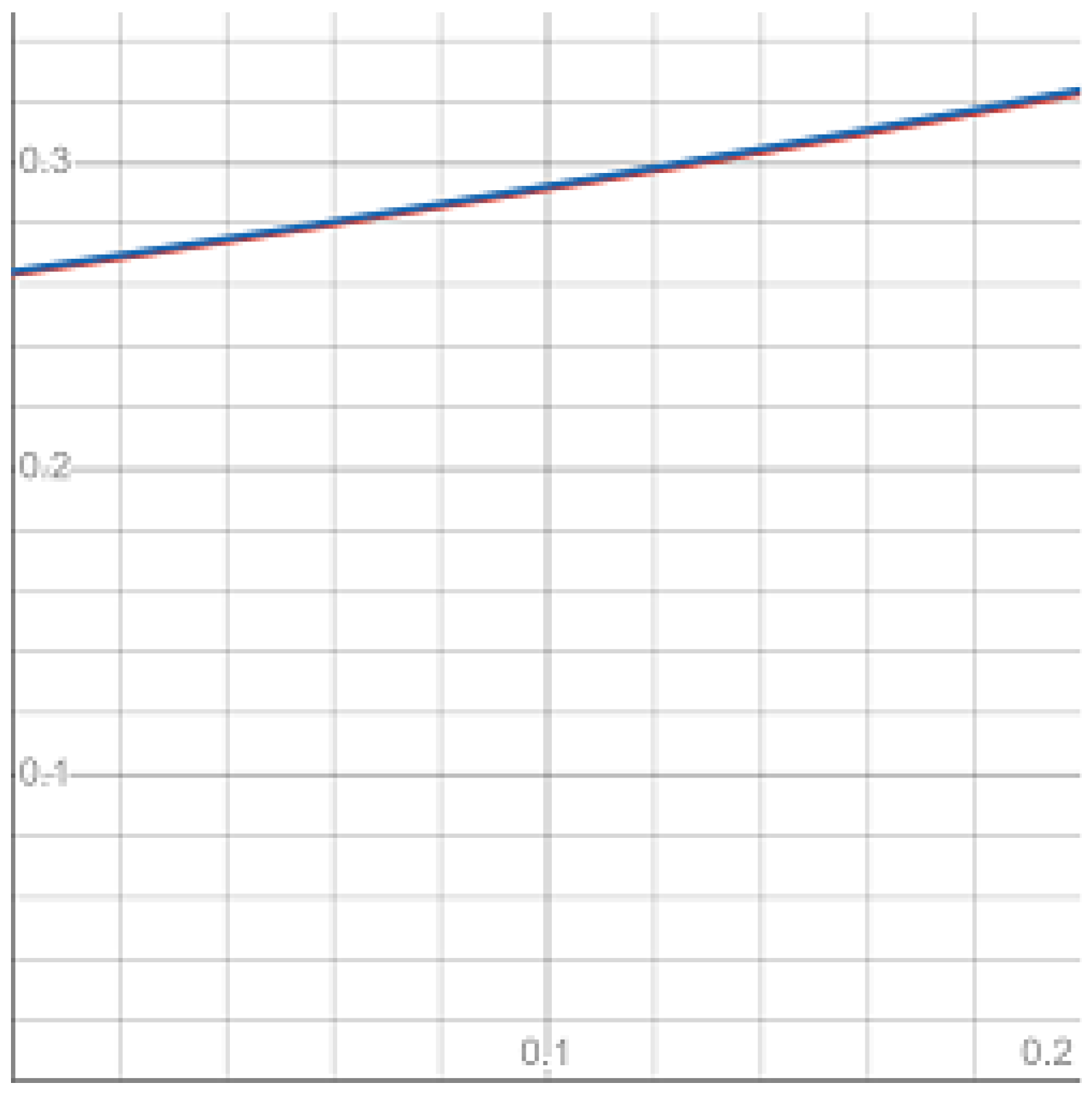
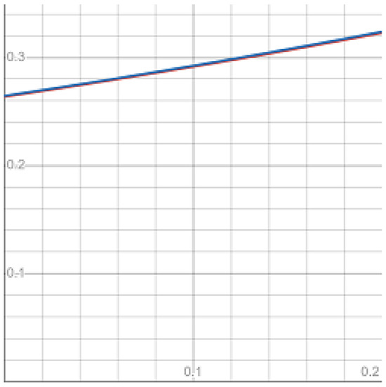
are plotted in Figure 1.

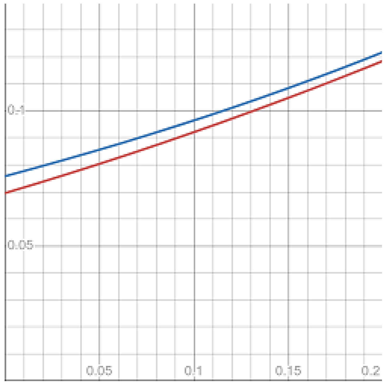
The second moments

$$\mathrm{E}{B}^2(t,1)=e^{\frac{(t-1)\left(5t^2-t+8\right)}{3}}\mathrm{and}\mathrm{E}{B}_{\mathrm{IG}}^2(t,1)=e^{\frac{t^2+4t-3}{2}-\sqrt{1+\frac{(1-t)(10t^2-5t+1)}{6}}}$$

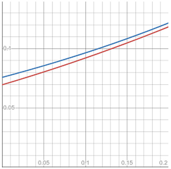
are given in Figure 2.

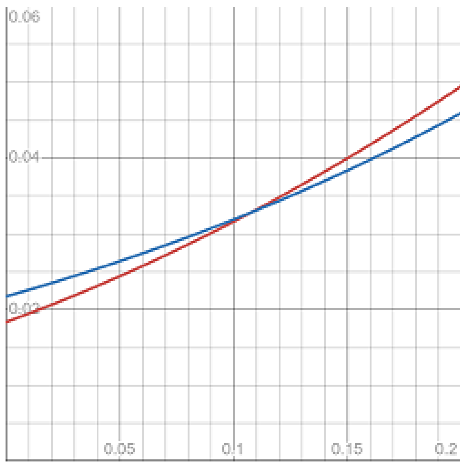
The third moments

$$\mathrm{E}{B}^3(t,1)=e^{2(t-1)\left(2t^2-t+2\right)}\mathrm{and}\mathrm{E}{B}_{\mathrm{IG}}^3(t,1)=e^{\frac{3t^2+12t-11}{4}-\sqrt{1+\frac{(1-t)(16t^2-11t+1)}{6}}}$$

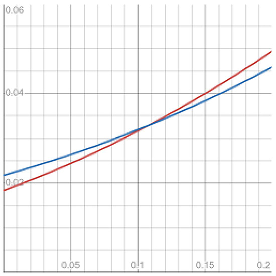
are provided in Figure 3.

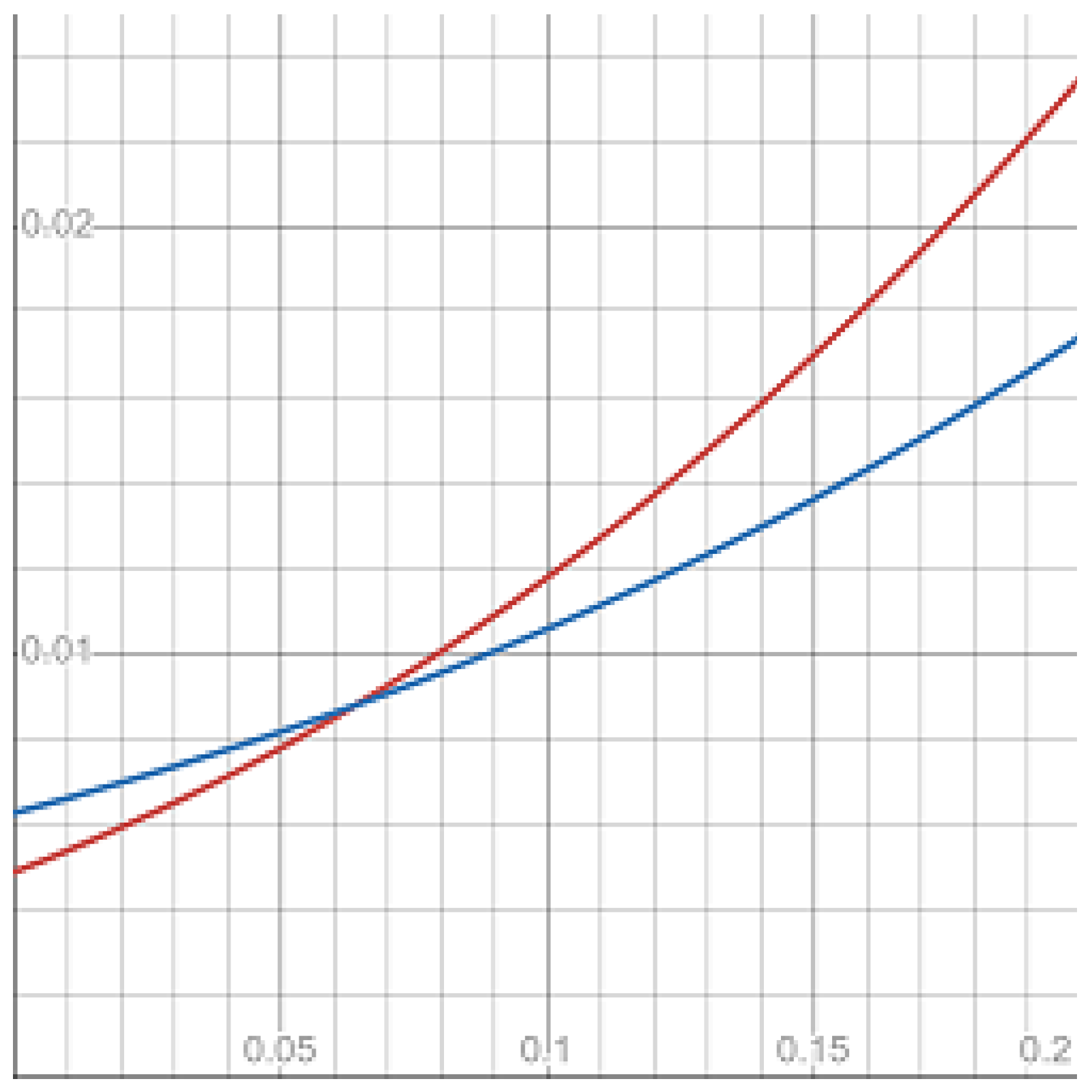
The fourth moments

$$\mathrm{E}{B}^4(t,1)=e^{\frac{2(t-1)\left(11t^2-7t+8\right)}{3}}\mathrm{and}\mathrm{E}{B}_{\mathrm{IG}}^4(t,1)=e^{t^2+4t-4-\sqrt{1+\frac{(1-t)(22t^2-17t+1)}{6}}}$$

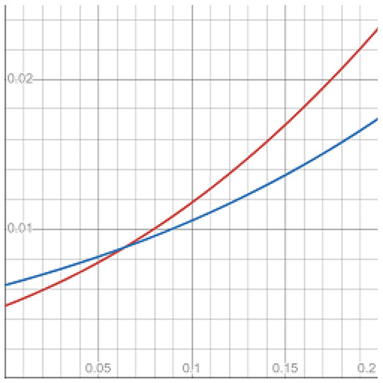
are plotted in Figure 4.

Table 3. The comparison of moments of the Gaussian and Gaussian IG Ho–Lee bond prices for $t\in [0,0.2]$ with step $0.025$ in Metric (29).

$\mathit{v}\mathit{\setminus }\mathit{t}$	0	0.025	0.05	0.075	0.1	0.125	0.15	0.175	0.2
1	$0.32$	$0.32$	$0.32$	$0.33$	$0.34$	$0.35$	$0.35$	$0.37$	$0.38$
2	$8.3$	$7.1$	$6.1$	$5.2$	$4.5$	$3.9$	$3.4$	$3.0$	$2.7$
3	$15.6$	$11.4$	$7.5$	$4.0$	$0.9$	$1.8$	$4.0$	$5.8$	$7.1$
4	$22.4$	$13.5$	$4.8$	$3.4$	$10.2$	$15.6$	$19.8$	$23.2$	$25.8$

compares the moments of bond prices in the metric

$$\mathrm{m}\left(v\right)=\frac{\left|\mathrm{E}{B}^v(t,1)-\mathrm{E}{B}_{\mathrm{IG}}^v(t,1)\right|}{max\left\{\mathrm{E}{B}^v(t,1),\mathrm{E}{B}_{\mathrm{IG}}^v(t,1)\right\}}100\%.$$

(29)

Finally, let us mention that the expressions for bond option prices in Theorem 2 and Corollary 1 are analogous to the formulas for stock derivatives with gamma and inverse gamma drift and volatility coefficients. As such, they can be computed by the same method as is used in the numerical examples in Section 4 in Ivanov [41].

4.4. Complex Example

As can be seen from (16), the moments of the GIG bond price do not exist when

$$2\rho (v,t)-{\eta }^2\ge 0.$$

(30)

Let

$$Z_1=Z_1\left(t\right)={(T-t)}^2{\int }_0^t{\sigma }_s^{2}ds$$

and

$$Z_2=Z_2\left(t\right)={\int }_t^T{\sigma }_s^2{(T-s)}^{2}ds-2{\int }_t^T(T-s){\theta }_{s}ds-2(T-t){\int }_0^t{\theta }_{s}ds.$$

Then, the inequality (30) has the form

$$Z_1{v}^2+Z_{2}v-{\eta }^2\ge 0$$

with $Z_1>0$.

The equation $Z_1{v}^2+Z_{2}v-{\eta }^2=0$ has roots

$$v_{1,2}=\frac{-Z_2\pm \sqrt{Z_2^2+4Z_1{\eta }^2}}{2Z_1}.$$

Therefore, if

$$v\ge v_2=\frac{\sqrt{Z_2^2+4Z_1{\eta }^2}-Z_2}{2Z_1}>0,$$

then Condition (30) is satisfied and

$$\mathrm{E}{B}_{\mathrm{GIG}}^v(t,T)=\infty ,v\ge v_2.$$

(31)

Identity (31) indicates that the GIG continuous Ho–Lee model, unlike the pure Gaussian one, permits infinite values for higher moments of the bond price. Therefore, the new model is able to distinguish, particularly, specific central parts of empirical distributions of the interest rates which cannot be well-fitted with the normal model.

5. Discussion

We have introduced a new model of the term structure of stochastic interest rates that is more flexible to the specification of real financial data than the continuous Ho–Lee one. The new model incorporates the drift and volatility coefficients, which depend in addition on the GIG distribution, which is very popular in financial modeling. This model is an example of the HJM model, and it allows the interest rate to be negative, as sometimes happens at practice (see Eberlein et al. [45] and Fontana et al. [60]).

Similar to the continuous-time Ho–Lee model, Theorem 1 provides us with the analytical expressions for the bond price and its moments in the GIG continuous Ho–Lee model. It should be noticed that the new model, unlike the continuous Ho–Lee one, permits infinite values for the bond price moments under some relations between the parameters. Employing the additional conditions on the parameters of the model, Theorem 2 and Corollary 1 give us the formulas for the prices of European call and put option written on bonds in the discussed framework. Analogous to the results of Ivanov [41] for stock options in the gamma and inverse gamma volatility models, the obtained expressions are determined by the values of the Humbert confluent hypergeometric function of two variables. The availability of these formulas enables us to estimate the implied parameters of the interest rate dynamic comparing the real market and model option prices.

In the numerical analysis section, we have compared the moments of bond prices in the new and continuous Ho–Lee models. Amid the GIG distributions, we choose, for the experiments, the inverse Gaussian ($\lambda =-0.5$) one. It appears that the third and fourth moments of the bond prices with very close means can differ significantly in the suggested metric (see Figure 1, Figure 2, Figure 3 and Figure 4 and Table 3). Also, we have provided a general condition on the parameters when the higher moments of the GIG bond price do not exist.

Future investigations can relate to the valuation of swap and exotic derivatives (see Chapters 12 and 13 in Musiela and Rutkowski [5]) in the new model. As is easy to see from Table 2 and the statement of Theorem 2, the results about the bond option pricing do not imply the HIG distribution, which is far-famed in financial applications. Therefore, the conditions of Theorem 2 could be relaxed in the ensuing studies. Moreover, we look forward for the extension of the GIG continuous Ho–Lee model to more general term structure models in the context of Table 1. First of all, the GIG Vasicek interest rate model should be developed and examined.

6. Conclusions

In this paper, we have defined and studied the new model of stochastic interest rate dynamics that generalizes the continuous Ho–Lee model by assuming that the drift and volatility coefficients depend also on the independent GIG distribution. The conducted research allows us to make the following conclusions:

• The proposed model is analytically tractable. We have found the closed-form expressions for the bond price, its moments, and the prices of European call and put bond options. However, the results related to the option prices are obtained under the special restrictions on the parameters of model;
• The numerical experiments have shown that the third and fourth moments of the continuous Ho–Lee and GIG continuous Ho–Lee bond prices with the same mean may differentiate at up to 15.6% and 25.8%, respectively. And the higher moments of the GIG bond price can take infinite values. Therefore, the compound model could better reflect the properties of market yield curves;
• In the next examinations, the call and put bond option prices could be found with fewer constraints on the parameters. The problem of swap and exotic derivative pricing in the new model should be discussed. The possibility of the extension of the introduced model to the GIG Vasicek model should be considered as well.

References

- Ho, T.S.Y.; Lee, S.B. Term structure movements and pricing interest rate contingent claims. J. Financ. 1986, 41, 1011–1029. [Google Scholar] [CrossRef]
- Hull, J.; White, A. Pricing interest-rate-derivative securities. Rev. Finan. Stud. 1990, 3, 573–592. [Google Scholar] [CrossRef]
- Heath, D.; Jarrow, R.; Morton, A. Bond pricing and the term structure of interest rate: A new methodology for contingent claims valuation. Econometrica 1992, 60, 77–105. [Google Scholar] [CrossRef]
- Subrahmanyam, M.G. The term structure of interest rates: Alternative approaches and their implications for the valuation of contingent claims. Geneva Pap. Risk Insur. Theory 1996, 21, 7–28. [Google Scholar] [CrossRef]
- Musiela, M.; Rutkowski, M. Martingale Methods in Financial Modelling, 2nd ed.; Springer: Berlin, Germany, 2005; pp. 331–337, 348–349, 381–412, 431–526. [Google Scholar]
- Halphen, É. Sur un nouveau type de courbe de fréquence. C. R. Hebdom. Séances Académ. Sc. 1941, 213, 634–635. [Google Scholar]
- Barndorff-Nielsen, O.E. Exponentially decreasing distributions for the logarithm of particle size. Proc. R. Soc. Lond. A 1977, 353, 401–419. [Google Scholar]
- Eberlein, E.; Keller, U. Hyperbolic distributions in finance. Bernoulli 1995, 1, 281–299. [Google Scholar] [CrossRef]
- Barndorff-Nielsen, O.E. Processes of normal inverse Gaussian type. Financ. Stoch. 1998, 2, 41–68. [Google Scholar] [CrossRef]
- Küchler, U.; Neumann, K.; Sørensen, M.; Streller, A. Stock returns and hyperbolic distributions. Math. Comput. Model. 1999, 29, 1–15. [Google Scholar] [CrossRef]
- Bauer, C. Value at risk using hyperbolic distributions. J. Econ. Bus. 2000, 52, 455–467. [Google Scholar] [CrossRef]
- Eriksson, A.; Ghysels, E.; Wang, F. The normal inverse Gaussian distribution and the pricing of derivatives. J. Deriv. 2009, 16, 23–37. [Google Scholar] [CrossRef]
- Luciano, E.; Marena, M.; Semeraro, P. Dependence calibration and portfolio fit with factor-based subordinators. Quant. Finan. 2016, 16, 1037–1052. [Google Scholar] [CrossRef]
- Fajardo, J.; Farias, A. Multivariate affine generalized hyperbolic distributions: An empirical investigation. Internat. Rev. Finan. Anal. 2009, 18, 174–184. [Google Scholar] [CrossRef]
- Daskalaki, S.; Katris, C. Marginal distribution modeling and value at risk estimation for stock index returns. J. Appl. Oper. Res. 2014, 6, 207–221. [Google Scholar]
- Rathgeber, A.W.; Stadler, J.; Stöckl, S. Fitting generalized hyperbolic processes—New insights for generating initial values. Commun. Stat. Simul. Comput. 2017, 46, 5752–5762. [Google Scholar] [CrossRef]
- Rathgeber, A.W.; Stadler, J.; Stöckl, S. Financial modelling applying multivariate Lévy processes: New insights into estimation and simulation. Phys. A Stat. Mech. Appl. 2019, 532, 121386. [Google Scholar] [CrossRef]
- Nakakita, M.; Nakatsuma, T. Bayesian analysis of intraday stochastic volatility models of high frequency stock returns with skew heavy tailed errors. J. Risk Finan. Manag. 2021, 14, 145. [Google Scholar] [CrossRef]
- Nakajima, J. Skew selection for factor stochastic volatility models. J. Appl. Stat. 2020, 47, 582–601. [Google Scholar] [CrossRef]
- Chan, S.; Chu, J.; Nadarajah, S.; Osterrieder, J. A statistical analysis of cryptocurrencies. J. Risk Finan. Manag. 2017, 10, 12. [Google Scholar] [CrossRef]
- Sheraz, M.H.M.; Dedu, S.A. Bitcoin cash: Stochastic models of fat-tail returns and risk modeling. Econ. Comput. Econ. Cyber. Stud. Res. 2020, 54, 43–58. [Google Scholar]
- Abraham, B.; Balakrishna, N.; Sivakumar, R. Gamma stochastic volatility models. J. Forecast. 2006, 25, 153–171. [Google Scholar] [CrossRef]
- Frühwirth-Schnatter, S.; Sögner, L. Bayesian estimation of stochastic volatility models based on OU processes with marginal Gamma law. Ann. Inst. Stat. Math. 2009, 61, 159–179. [Google Scholar] [CrossRef]
- James, L.F.; Müller, G.; Zhang, Z. Stochastic volatility models based on OU-gamma time change: Theory and estimation. J. Busin. Econ. Stat. 2018, 36, 75–87. [Google Scholar] [CrossRef]
- Nzokem, A.H. Pricing European options under stochastic volatility models: Case of five-parameter variance-gamma process. J. Risk Finan. Manag. 2023, 16, 55. [Google Scholar] [CrossRef]
- Fung, T.; Seneta, E. Modelling and estimation for bivariate financial returns. Int. Stat. Rev. 2010, 78, 117–133. [Google Scholar] [CrossRef]
- Liu, J. A Bayesian semiparametric realized stochastic volatility model. J. Risk Finan. Manag. 2021, 14, 617. [Google Scholar] [CrossRef]
- Nakajima, J.; Omori, Y. Stochastic volatility model with leverage and asymmetrically heavy-tailed error using GH skew Student’s t-distribution. Comput. Stat. Data Anal. 2012, 56, 3690–3704. [Google Scholar] [CrossRef]
- Men, Z.; Wirjanto, T.S.; Kolkiewicz, A.W. Multiscale stochastic volatility model with heavy tails and leverage effects. J. Risk Finan. Manag. 2021, 14, 225. [Google Scholar] [CrossRef]
- Takahashi, M.; Watanabe, T.; Omori, Y. Forecasting daily volatility of stock price index using daily returns and realized volatility. Econom. Stat. 2024, 32, 34–56. [Google Scholar] [CrossRef]
- Eberlein, E.; von Hammerstein, E.A. Generalized hyperbolic and inverse Gaussian distributions: Limiting cases and approximation of processes. In Seminar on Stochastic Analysis, Random Fields and Applications IV, Progress in Probability; Dalang, R.C., Dozzi, M., Russo, F., Eds.; Birkhäuser Verlag: Berlin, Germany, 2004; Volume 58, pp. 221–264. [Google Scholar]
- Ivanov, R.V. The semi-hyperbolic distribution and its applications. Stats 2023, 6, 1126–1146. [Google Scholar] [CrossRef]
- Maltsev, V.; Pokojovy, M. Applying Heath-Jarrow-Morton model to forecasting the US treasury daily yield curve rates. Mathematics 2021, 9, 114. [Google Scholar] [CrossRef]
- Tóth-Lakits, D.; Arató, M. On the calibration of the Kennedy model. Mathematics 2024, 12, 3059. [Google Scholar] [CrossRef]
- Fontana, C.; Lanaro, G.; Murgoci, A. The geometry of multi-curve interest rate models. Quantit. Finance 2024, 1–20, in print. [Google Scholar] [CrossRef]
- Gardini, M.; Santilli, E. A Heath-Jarrow-Morton framework for energy markets: Review and applications for practitioners. Decisions Econom. Finan. 2024, 1–40, in print. [Google Scholar] [CrossRef]
- Hull, J.; White, A. One-factor interest-rate models and the valuation of interest-rate derivative securities. J. Financ. Quant. Anal. 1993, 28, 235–254. [Google Scholar] [CrossRef]
- Serafin, T.; Michalak, A.; Bielak, L.; Wylomańska, A. Averaged-calibration-length prediction for currency exchange rates by a time-dependent Vasicek model. Theor. Econ. Lett. 2020, 10, 579–599. [Google Scholar] [CrossRef]
- Orlando, G.; Bufalo, M. Interest rates forecasting: Between Hull and White and the CIR#—How to make a single-factor model work. J. Forecast. 2021, 40, 1566–1580. [Google Scholar]
- van der Zwaard, T.; Grzelak, L.A.; Oosterlee, C.W. On the Hull-White model with volatility smile for valuation adjustments. arXiv 2024, arXiv:2403.14841. [Google Scholar] [CrossRef]
- Ivanov, R.V. On the stochastic volatility in the generalized Black-Scholes-Merton model. Risks 2023, 11, 111. [Google Scholar] [CrossRef]
- Madan, D.B.; Carr, P.; Chang, E.C. The variance gamma process and option pricing. Rev. Finan. 1998, 2, 79–105. [Google Scholar] [CrossRef]
- Ano, K.; Ivanov, R.V. On exact pricing of FX options in multivariate time-changed Lévy models. Rev. Deriv. Res. 2016, 19, 201–216. [Google Scholar]
- Ivanov, R.V. On properties of the hyperbolic distribution. Mathematics 2024, 12, 2888. [Google Scholar] [CrossRef]
- Eberlein, E.; Gerhart, C.; Grbac, Z. Multiple curve Lévy forward price model allowing for negative interest rates. Math. Finan. 2020, 30, 167–195. [Google Scholar] [CrossRef]
- Orlando, G.; Taglialatela, G. A review on implied volatility calculation. J. Comput. Appl. Math. 2017, 320, 202–220. [Google Scholar] [CrossRef]
- Merton, R.C. Theory of rational option pricing. Bell J. Econom. Manag.Sci. 1973, 4, 141–183. [Google Scholar] [CrossRef]
- Shiryaev, A.N. Essentials of Stochastic Finance; World Scientific: Singapore, 1999; pp. 792–799. [Google Scholar]
- Barndorff-Nielsen, O.E.; Halgreen, C. Infinite divisibility of the hyperbolic and generalized inverse Gaussian distributions. Z. Wahrscheinlichkeitstheorie Verw. Geb. 1977, 38, 309–312. [Google Scholar] [CrossRef]
- Gradshteyn, I.S.; Ryzhik, I.M. Table of Integrals, Series and Products, 7th ed.; Elsevier Academic Press: New York, NY, USA, 2007; pp. 368, 925. [Google Scholar]
- Jørgensen, B. Statistical Properties of the Generalized Inverse Gaussian Distribution; Springer: New York, NY, USA, 1982; pp. 5–19, 39–65. [Google Scholar]
- Barndorff-Nielsen, O.E. Hyperbolic distributions and distributions on hyperbolae. Scand. J. Statist. 1978, 5, 151–157. [Google Scholar]
- Blaesild, P. Conditioning with conic sections in the two-dimensional normal distribution. Ann. Stat. 1979, 7, 659–670. [Google Scholar] [CrossRef]
- Shreve, S.E. Stochastic Calculus for Finance II Continuous-Time Models; Springer: New York, NY, USA, 2004; pp. 124–128. [Google Scholar]
- Eberlein, E. Application of generalized hyperbolic Lévy motions to finance. In Lévy Processes; Barndorff-Nielsen, O.E., Resnick, S.I., Mikosch, T., Eds.; Birkhäuser: Boston, MA, USA, 2001; pp. 319–336. [Google Scholar]
- Brigo, D.; Mercurio, F. Interest Rate Models—Theory and Practice, 2nd ed.; Berlin: Springer, Germany, 2006; pp. 39–40. [Google Scholar]
- Srivastava, H.M.; Karlsson, W. Multiple Gaussian Hypergeometric Series; Ellis Horwood Limited: New York, NY, USA, 1985; p. 25. [Google Scholar]
- Humbert, P. The confluent hypergeometric functions of two variables. Proc. R. Soc. Edinb. 1922, 41, 73–96. [Google Scholar] [CrossRef]
- Bateman, H.; Erdélyi, A. Higher Transcendental Functions; McGraw-Hill: New York, NY, USA, 1953; Volume I, pp. 222–247. [Google Scholar]
- Fontana, C.; Gnoatto, A.; Szulda, G. Multiple yield curve modelling with CBI processes. Math. Finan. Econom. 2021, 15, 579–610. [Google Scholar] [CrossRef]
Disclaimer/Publisher’s Note: The statements, opinions and data contained in all publications are solely those of the individual author(s) and contributor(s) and not of MDPI and/or the editor(s). MDPI and/or the editor(s) disclaim responsibility for any injury to people or property resulting from any ideas, methods, instructions or products referred to in the content. |
© 2025 by the author. Licensee MDPI, Basel, Switzerland. This article is an open access article distributed under the terms and conditions of the Creative Commons Attribution (CC BY) license (https://creativecommons.org/licenses/by/4.0/).