Deep Multi-Component Neural Network Architecture

Abstract

Existing neural network architectures often struggle with two critical limitations: (1) information loss during dataset length standardization, where variable-length samples are forced into fixed dimensions, and (2) inefficient feature selection in single-modal systems, which treats all features equally regardless of relevance. To address these issues, this paper introduces the Deep Multi-Components Neural Network (DMCNN), a novel architecture that processes variable-length data by regrouping samples into components of similar lengths, thereby preserving information that traditional methods discard. DMCNN dynamically prioritizes task-relevant features through a component-weighting mechanism, which calculates the importance of each component via loss functions and adjusts weights using a SoftMax function. This approach eliminates the need for dataset standardization while enhancing meaningful features and suppressing irrelevant ones. Additionally, DMCNN seamlessly integrates multimodal data (e.g., text, speech, and signals) as separate components, leveraging complementary information to improve accuracy without requiring dimension alignment. Evaluated on the Multimodal EmotionLines Dataset (MELD) and CIFAR-10, DMCNN achieves state-of-the-art accuracy of 99.22% on MELD and 97.78% on CIFAR-10, outperforming existing methods like MNN and McDFR. The architecture’s efficiency is further demonstrated by its reduced trainable parameters and robust handling of multimodal and variable-length inputs, making it a versatile solution for classification tasks.

1. Introduction

1.1. Research Background

Deep learning has revolutionized the field of artificial intelligence by providing a natural way to extract meaningful feature representations from raw data without relying on hand-crafted descriptors. Feature extraction plays a critical role in various applications, as it reduces input dimensionality [1] while enabling a more meaningful representation that uncovers underlying patterns and relationships. Representation learning, a cornerstone of deep learning, significantly enhances the ability to extract useful information when building classifiers or other predictors [2]. A good representation not only captures the posterior distribution of the underlying data but also serves as a foundation for achieving superior predictive results. Over the years, numerous architectures have been proposed to address challenges such as overfitting, information loss during dataset preprocessing, and the need to extract the most informative features while ignoring irrelevant ones.

1.2. Literature Review

Despite significant advancements, many existing architectures still face limitations. Convolutional Neural Networks (CNNs), for instance, are widely regarded as powerful tools for feature extraction but struggle to capture spatial relationships between elements in images [3]. For example, a CNN might misidentify a randomly arranged face with misplaced eyes, ears, and nose as a valid human face. To address this issue, Sabour et al. introduced Capsule Networks (CapsNet) in 2017 [4]. While CapsNets excel at defining location relationships between features in deep neural networks, they remain computationally expensive and unsuitable for mobile devices [5]. Other approaches, such as Vision Transformers (ViTs) and Binary Neural Networks (BNNs), have shown promise but often require extensive computational resources or specialized training techniques [6,7]. These limitations highlight the need for innovative architectures to overcome existing challenges while maintaining simplicity and efficiency.

1.3. Main Contributions

This paper introduces the Deep Multi-Components Neural Network Architecture (DMCNN), a novel approach designed to address several critical issues in deep learning. The key contributions of this work are as follows:

• Avoiding Overfitting: DMCNN effectively mitigates overfitting by leveraging a multi-component architecture that enhances important features while reducing the weight of unimportant ones.
• Multimodal Input Handling: Unlike traditional models, DMCNN integrates multimodal data (e.g., speech, text, and signals) as additional components, using complementary information to achieve higher accuracy.
• Dimension Flexibility: DMCNN eliminates the need for standardizing input lengths, making it suitable for datasets with varying dimensions.
• Feature Selection: The architecture dynamically identifies and prioritizes the most informative features, ensuring optimal classification performance with minimal trainable parameters.

State-of-the-Art Performance: Experimental results demonstrate that DMCNN surpasses relevant state-of-the-art methods, achieving an accuracy of 99.22% on the MELD dataset [8,9] and 97.78% on the CIFAR-10 dataset [2].

1.4. Paper Structure

The remainder of this paper is organized as follows:

-

Section 2: Provides an overview of related works, discussing existing architectures and their limitations.

-

Section 3: Describes the proposed methodology in detail, including the architecture and mathematical formulations.

-

Section 4: Presents the experimental setup, results, and comparisons with prior works.

-

Section 5: Concludes the paper with a summary of findings and potential directions for future research.

2. Related Works

Deep learning architectures have evolved significantly to address various challenges in feature extraction, classification, and multimodal data integration. In this section, we review existing approaches and highlight their strengths and limitations. The discussion is divided into the following subsections: Multimodal Architectures, Vision Transformers, Binary Neural Networks, Nesting Transformers, and Other Relevant Models.

2.1. Multimodal Architectures

Several neural network architectures have been proposed to process multimodal data by extracting generic yet descriptive features. Among these, the Meaningful Neural Network (MNN) [8,9] and Multichannel Deep Feature Representation (McDFR) [1] are notable examples. These architectures rely on unsupervised learning for generic feature extraction, followed by supervised learning for class-specific features. However, our proposed architecture differs by using supervised learning for both generic and class-specific features. This approach enhances important features while reducing irrelevant ones, resulting in superior performance. Experimental results demonstrate that Deep Multi-Components Neural Network (DMCNN) outperforms MNN [8,9] and McDFR [1].

2.2. Vision Transformers

Vision Transformers (ViTs) have gained significant attention for image classification tasks. Jeevan and Sethi [6] introduced Vision X-formers (ViXs), which address the quadratic bottleneck of traditional ViTs by incorporating linear attention mechanisms, convolutional layers, and Rotary Position Embedding (RoPE). These modifications improved classification accuracy to 79.50% on the CIFAR-10 dataset [2]. Similarly, Dosovitskiy et al. [10] proposed a transformer-based model that treats images as sequences of patches, achieving state-of-the-art results on large-scale datasets. Despite their success, ViTs often require significant computational resources and large datasets for training.

2.3. Binary Neural Networks

Binary Neural Networks (BNNs) have been explored to reduce computational costs while maintaining competitive performance. Chen et al. [7] demonstrated that BNNs can be trained without batch normalization (BN-Free), achieving 92.08% accuracy on CIFAR-10 [2]. Additionally, GradInit [7], a heuristic-based initialization method, accelerates convergence and improves test performance for convolutional architectures, achieving 94.71% accuracy on CIFAR-10 [2]. While BNNs offer efficiency, they may still lag behind full-precision models in terms of accuracy.

2.4. Nesting Transformers

Han and Long [11] proposed NesT, a novel approach that nests basic local transformers on non-overlapping image blocks and aggregates them hierarchically. This method requires less training data and achieves 96% accuracy on CIFAR-10 [2], with only 6 million parameters. NesT demonstrates the potential of hierarchical architectures for efficient generalization. Similarly, Deng and Feng [12] introduced an adaptive replica-exchange stochastic gradient Markov Chain Monte Carlo (SGMCMC) method, achieving 97.42% accuracy on CIFAR-10 [2]. These advancements highlight the importance of hierarchical and adaptive strategies in deep learning.

2.5. Other Relevant Models

Several other models have contributed to advancements in image classification and multimodal processing. For example:

-

XnODR and XnIDR: Sun and Fard [5] proposed two new classes of fully connected layers, achieving 95.32% accuracy on CIFAR-10 [2].

-

CutMix: Yun and Han [13] introduced CutMix, a regularization strategy that mixes patches from training images, achieving 97.12% accuracy on CIFAR-10 [2].

-

Neuronal Architecture Transfer: Lu et al. [14] proposed an evolutionary search routine and accuracy predictor, achieving 97.40% accuracy on CIFAR-10 [2].

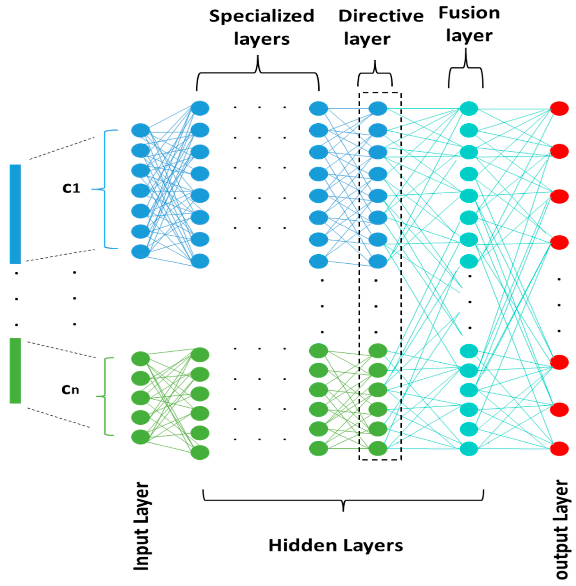
3. Materials and Methods

The Meaningful Neural Network (MNN) [8,9] is a novel neural network model developed by H. Filali, J. Riffi, and C. Boulealam in 2022 [8,9] that enables learning features from various architectures, methods, and descriptive vectors to meaningfully represent input from many modalities, such as voice, image, and text. The primary concept behind MNN [8,9] is to designate a section of this network called (specialist layers) for learning each input vector component. The latter’s traits are in fact learned independently in a considerable way. Three different sorts of layers make up the MNN [8,9] architecture, as seen in Figure 1.

3.1. Specialized Layers

Each of these layers has a group of neurons that are trained to extract and learn the representations of the input vector components that are stored within. According to the number of components in the input vector, we can often have any number of neuron sets. The following formula can be used to calculate the weights and update them throughout the gradient backpropagation step:

• Forward Propagation:

$$z_j^{c\left(l\right)}=\Psi (\sum _{k=1}^{T_{(l-1)}}{w}_{\left(kj\right)}^{\left(l\right)}{a}_k^{(l-1)}+b_j^{\left(l\right)})$$

(1)

• Backward Propagation:

During backpropagation, each component updates its weights based on the fusion layer, which contains all the updated weights. The fusion layer integrates the features from all components, ensuring that the weight updates in the fusion layer are based on all components. This process ensures that each component’s weight is updated with consideration of the other components. As a result, each component receives the correct weight updates, enhancing the accuracy of each component. This collaborative updating mechanism ultimately leads to improved accuracy in the final classification performed by the fusion component.

$${\delta }_j^{c\left(l\right)}={\sigma }^{\prime }(z_j^l) \ast \sum _{k=1}^{n(l+1)}{w}_{\left(jk\right)}^{(l+1)}{\delta }_k^{(l+1)}$$

(2)

$${\displaystyle \frac{\mathsf{\partial }E}{\mathsf{\partial }{w}_{\left(ij\right)}^{c\left(l\right)}}}=a_i^{c(l-1)}{\delta }_j^{c\left(l\right)}$$

(3)

$${\displaystyle \frac{\mathsf{\partial }\mathrm{E}}{\mathsf{\partial }{\mathrm{b}}_{\mathrm{j}}^{\mathrm{c}\left(\mathrm{l}\right)}}}={\mathsf{\delta }}_{\mathrm{j}}^{\mathrm{c}\left(\mathrm{l}\right)}$$

(4)

3.2. Directive Layer

One directive layer is present in the suggested architecture. While the other side is fully attached, the left side is just partly connected. By taking into consideration the two sets of neurons for the specialized layers, this layer enables the control of error propagation.

• Forward Propagation:

$$z_j^{c\left(l\right)}=\Psi (\sum _{k=1}^{T_{(l-1)}}{w}_{\left(kj\right)}^{\left(l\right)}{a}_k^{(l-1)}+b_j^{\left(l\right)})$$

(5)

• Backward Propagation:

$${\delta }_j^{c\left(l\right)}={\sigma }^{\prime }(z_j^l) \ast \sum _{k=1}^{n(l+1)}{w}_{\left(jk\right)}^{(l+1)}{\delta }_i^{(l+1)}$$

(6)

$${\displaystyle \frac{\mathsf{\partial }E}{\mathsf{\partial }{w}_{\left(ij\right)}^{c\left(l\right)}}}=a_i^{c(l-1)}{\delta }_j^{c\left(l\right)}$$

(7)

$${\displaystyle \frac{\mathsf{\partial }E}{\mathsf{\partial }{b}_j^{c\left(l\right)}}}={\delta }_j^{c\left(l\right)}$$

(8)

3.3. Fusing Layer

This layer is completely connected. It enables the merging of learned representations from earlier levels.

• Forward Propagation:

$$z_J^{c\left(l\right)}=\Psi (\sum _{k=1}^{T_{(l-1)}}{w}_{\left(kj\right)}^{\left(l\right)}{a}_k^{(l-1)}+b_j^{\left(l\right)})$$

(9)

• Backward Propagation:

$${\delta }_i^{c\left(l\right)}={\sigma }^{\prime }(z_j^l) \ast \sum _{k=1}^{n(l+1)}{w}_{\left(jk\right)}^{(l+1)}{\delta }_k^{(l+1)}$$

(10)

$${\displaystyle \frac{\mathsf{\partial }E}{\mathsf{\partial }{w}_{\left(ij\right)}^{c\left(l\right)}}}=a_i^{c(l-1)}{\delta }_j^{c\left(l\right)}$$

(11)

$${\displaystyle \frac{\mathsf{\partial }E}{\mathsf{\partial }{b}_j^{c\left(l\right)}}}={\delta }_j^{c\left(l\right)}$$

(12)

4. Proposed Architecture for DMCNN

Our proposed approach is based on two main steps: extracting features and fusing components. Before presenting the formal architecture, we need to distinguish the two types of layers that the proposed Neural Network Architecture contains:

4.1. Specialized Layers

The Specialized Layers are a foundational innovation of the DMCNN architecture, designed to address two critical limitations of traditional neural networks: information loss due to dataset length standardization and inefficient feature extraction. Unlike conventional architectures that force variable-length inputs into fixed dimensions (e.g., resizing images or truncating text sequences), DMCNN processes components of the input data without altering their original lengths. Each Specialized Layer is dedicated to processing a distinct component of the input vector (e.g., facial regions in images, audio segments, or text snippets).

4.2. Enhancing Important Features (Not a Layer)

This part is paramount in the modifications performed on the MNN [8,9] architecture. It consists of the following steps. First, the number of units in the output layer of each component must be equal to the number of classes. Second, we calculate the cost of each component to identify those with the best features from the others. Third, we calculate the weight of each component by putting the component’s cost value’s opposite in the vector to apply SoftMax of each value of the vector, The result is a vector representing the weights of all components, which is calculated using the following equation:

$$W\left(c\right)=SoftMax(1/\mathrm{c}\mathrm{o}\mathrm{s}t (c\left)\right)$$

(13)

where $c$ is the indices of the component and $W$ is the weight vector.

Next, we multiply the weight of each component with its output layer, and we consider the following parameters, as shown in Figure 1. Then, we define the proposed architecture for DMCNN in Figure 2.

• vol: vector output layer
• c: indices of component
• $W$: weight vector
• n: $len\left(W\right)$ is the length of a vector W refers to the number of components
• threshold: $1/n$$W\left(c\right)$: $Softmax(1/\mathrm{c}\mathrm{o}\mathrm{s}t(c\left)\right)$

The formula for the SoftMax function is as follows:

$$Softmax(x_i)={\displaystyle \frac{e^{\left(x_i\right)}}{sum\left(e^{\left(x_j\right)}\right)}} for all j$$

(14)

where x is the input vector, i is the index of the current element, and j is the index of all elements in the vector.

4.3. Fusing Layer

A fully connected layer that dynamically aggregates representations from the Specialized Layers using a novel weighting mechanism. Unlike traditional fusion methods that treat all components equally, DMCNN assigns weights based on each component’s relevance to the task. This innovation addresses the problem of inefficient feature selection in single-modal and multimodal systems.

4.4. Extraction Component

4.4.1. Case 1: A Multimodality

To explain the extraction process of the features using DMCNN, we consider a multimodal dataset $X$ containing $m$ modalities$X=\left\{M_1,M_2,\dots ,M_m\right\}$. Then, we take a modality ${M_i}_{\left(q_i,s_i\right)}=\left(y_1,y_2,\dots ,y_{q_i}\right)$ and feed it to component $C_i$, where $q_i$ is the number of examples and $s_i$ is the number of features. In each component, the features are extracted from each element $\left\{y_j\in M_i/i\in 1\dots m,j\in 1\dots q_i\right\}$ with what distinguishes it from its peers, $y_1,y_2,\dots ,y_{q_i}$. This operation occurs for all modalities in the dataset $X$.

4.4.2. Case 2: A Single Modality

The $X=M_{\left(q,s\right)}=\left\{{X_1}_{\left(1,s\right)},{X_2}_{\left(1,s\right)},\dots ,{X_q}_{\left(1,s\right)}\right\}$ modality dataset, where $q$ is the number of examples and $s$ is the number of features, is fed as a multi-component. Afterward, this changes the number of features of each element ${X_i}_{\left(1,s\right)}\in X$ in the dataset $X$ into $n$ new elements ${M_{.j}}_{\left(q,d_j\right)}=\left\{y_{ij}/i\in 1\dots q,j\in 1\dots n\right\}$, with a new number of features. Thus, the dataset becomes $X=\left\{{M_{.1}}_{\left(q,d_1\right)},{M_{.2}}_{\left(q,d_2\right)},\dots ,{M_{.n}}_{\left(q,d_n\right)}\right\}$, where each element $\left\{{y_{ij}}_{\left(1,d_j\right)}\in {M_{.j}}_{\left(1,s\right)}/i\in 1\dots q,j\in 1\dots n\right\}$ carries the characteristics of the original element as ${X_i}_{\left(1,s\right)}$, where $n$ is the number of components, ${\sum }_1^n{d}_i=s$, and $d_i$ is the number of features of $\left\{{y_{ij}}_{\left(1,d_i\right)}={M_j}_{\left(1,d_j\right)}\right\}$.

For each component $y_j$, the neural network extracts its features based on the differences, distinguishing it from every similar element in the new element of the original element of the dataset. For example, the similar items of $\left\{y_{1j}\in M_{.j}/i\in 1\dots q,j\in 1\dots n\right\}$ are $y_{2j},y_{3j},\dots ,y_{qj}\in M_{.j}.$This operation occurs for all the elements of $X=\left\{M_1,M_2,\dots ,M_n\right\}$ of the dataset.

This strategy is similar to that of the CNN [3], which considers the characteristics of each part of a single image. Consequently, this scheme makes our model more powerful in extracting the features of each element in a way that distinguishes it from all the others. Additionally, after we combine these features in the fusion component as features of the original item, we extract, in the fusion component, the distinctive properties of these features. Ultimately, the proposed model has indeed proved itself mostly accurate in classification.

As an illustration, consider a face image, as the original item carries the features of this image. After feeding this image to DMCNN, each component takes a portion of the facial features. The first component takes the features of the eye or a part of the eye or a part of the eye and the nose. The second component takes on the features of the ears or a part of them. The third component takes the features of the nose or a part of it, etc. Subsequently, each component extracts features of the new element $\left\{y_{1j}\in M_{.j}/i\in 1\dots q,j\in 1\dots n\right\}$ by what distinguishes it from its similar other elements $y_{2j},y_{3j},\dots ,y_{qj}\in M_{.j},$. This extraction process is performed on every element in each component. As a result, each component carries the features of the new element, which is originally part of the features of the original element $X_i$.

Before we gathered all the components in the fusion component, we calculated the cost of each one by determining the appropriate loss function. This determined the component that carries the most important features of the $j^{th}$ element $M_j$, which eventually means extracting the best features and ignoring the unimportant ones. Therefore, to accomplish this task, we need to calculate the weight from its cost and multiply it by the output vector of that component, as shown in Figure 3.

Figure 4 illustrates the process of calculating each component’s weight in DMCNNA for effective feature combination.

4.5. Fusion Component

4.5.1. Case 1: A Multimodality

In this next step, we combine the output of each component into the fusion component. Under the single modality, we see more details on how to combine the output features of each component.

4.5.2. Case 2: A Single Modality

We combine the output of each component into the fusion component by recombining the features of a new element $\left(y_{i_1},y_{i_2},\dots ,y_{i_n}\right)$, which constitutes the original element ${X_i}_{\left(1,s\right)}$. Subsequently, each element ${X_i}_{\left(1,s\right)}$ acquires good properties that distinguish it from the rest of the elements $\left\{{M_{.1}}_{\left(1,s\right)},{M_{.2}}_{\left(1,s\right)},\dots ,{M_{.n}}_{\left(1,s\right)}\right\}$ excluding the $i^{th}$ in the dataset, and this process happens to all of the other elements. Afterward, the fusion component extracts the features of the original element.

In this regard, back to the example presented earlier, the fusion component comes to extract the features of the image (the whole face). In this way, the proposed approach becomes more accurate in classification, where the power of DMCNN is mainly perceived in extracting the smallest details of the component among all others.

Furthermore, to achieve optimal results, the number of components chosen should be relatively large, corresponding to the number of features in the dataset.

5. Experimental Findings and Comparisons

5.1. Computational Environment

Our proposed model was implemented using the Python 3.8 Toolbox. The experiments were executed on an MSI As desktop with 12 GB RAM, core i7-5700 CPU 2.7 GHZ, NVIDIA GeForce GTX 970M, (NVIDIA, Santa Clara, CA, USA), 3 GB, and Windows 10 pro as operating system. Additionally, the model was trained using Google Collab.

5.2. Dataset

5.2.1. Multimodal

The Multimodal EmotionLines Dataset (MELD) [15,16] is an extension and enhancement of EmotionLines. MELD [15,16] contains about 13,000 utterances from 1433 dialogues from the TV series Friends. Each utterance is annotated with emotion and sentiment labels and encompasses audio, visual, and textual modalities datasets (text, audio, dual format). We fed it to our DMCNN model as three components: text in the first component; audio in the second component; and, finally, bimodal in the last component. We used an 80–20 split for training and testing, respectively, to ensure a robust evaluation of the model’s performance.

5.2.2. A Single Modality

As mentioned earlier, DMCNN can be applied also on one modality as multi-components by dividing the vector features into several ones of the same sample. This process is extensionally exhibited for all the samples. Then, it will be fed to the DMCNN model.

The number by which the feature vector should be divided is a little larger. It depends on the length of the vector features and the type of data set. For better accuracy, it is better to choose a number greater than 3.

The CIFAR-10 [2] dataset was used for the experiments of Krizhevsky. Since the image size is 32 × 32 × 3, we have a sequence length of 3074. We used CNN [3] to extract features and reduce the data input dimensionality to 128. Notably, our architecture contains 6 components; each of them has 2 layers and 0 dropouts to ensure uniformity in comparison with previous studies. Moreover, it uses the same projection for keys and values in Linformer. On the other side, the Adam optimizer, with $\alpha =0.001$ (learning rate), ${\beta }_1=0.9$, and ${\beta }_2=0.999$, was used for computing running averages of gradient and its square$. ϵ={10}^{-8}$, and 0.01 was used as the weight decay coefficient. We used the CPU privately in Google Collab. On the other hand, CPU usage for a batch size of 512 was reported, along with the top 1% and top 5% accuracy from the best of 3 runs.

In the CNN [3] model, we used four convolutional layers with 32, 32, 64, and 64 3 × 3 kernels, respectively, in each stage, with a stride of one and padding set to “same”.

We also fed 22, 22, 22, 22, 22, and 18 as input lengths, respectively, into each component.

5.3. Evaluation Metrics

The accuracy, top 1 accuracy, top 5 accuracy, precision, recall, and F1 score were the evaluation metrics we used to assess the performance of our model. The following is how these metrics are expressed:

Accuracy is the most straightforward performance metric; it just compares the proportion of accurately predicted observations to all observed.

$${\displaystyle \frac{TP+TN}{TP+FN+TN+FP}}$$

Top 1 accuracy is the conventional accuracy, which means that the model answer (the one with the highest probability) must be exactly the expected answer.

Top 5 accuracy means that any of the five highest-probability answers provided by the model must match the expected answer.

Recall is a metric for how well a model detects true positives.

$${\displaystyle \frac{TP}{TP+FN}}$$

Precision is the ratio of accurately anticipated positive observations to all observations made in the actual class, and the answer is yes.

$${\displaystyle \frac{TP}{TP+FP}}$$

F1-score is the average of precision and recall, weighted:

$$2{\displaystyle \frac{\mathit{Precision}\ast \mathit{Recall}}{\mathit{Precision}+\mathit{Recall}}}$$

where TP, TN, FP, and FN represent respectively the true positive, true negative, false positive, and false negative.

We also developed macro average and weighted average metrics, mounted cost, training accuracy, and training accuracy/validation accuracy curves according to epochs and showed the confusion matrix.

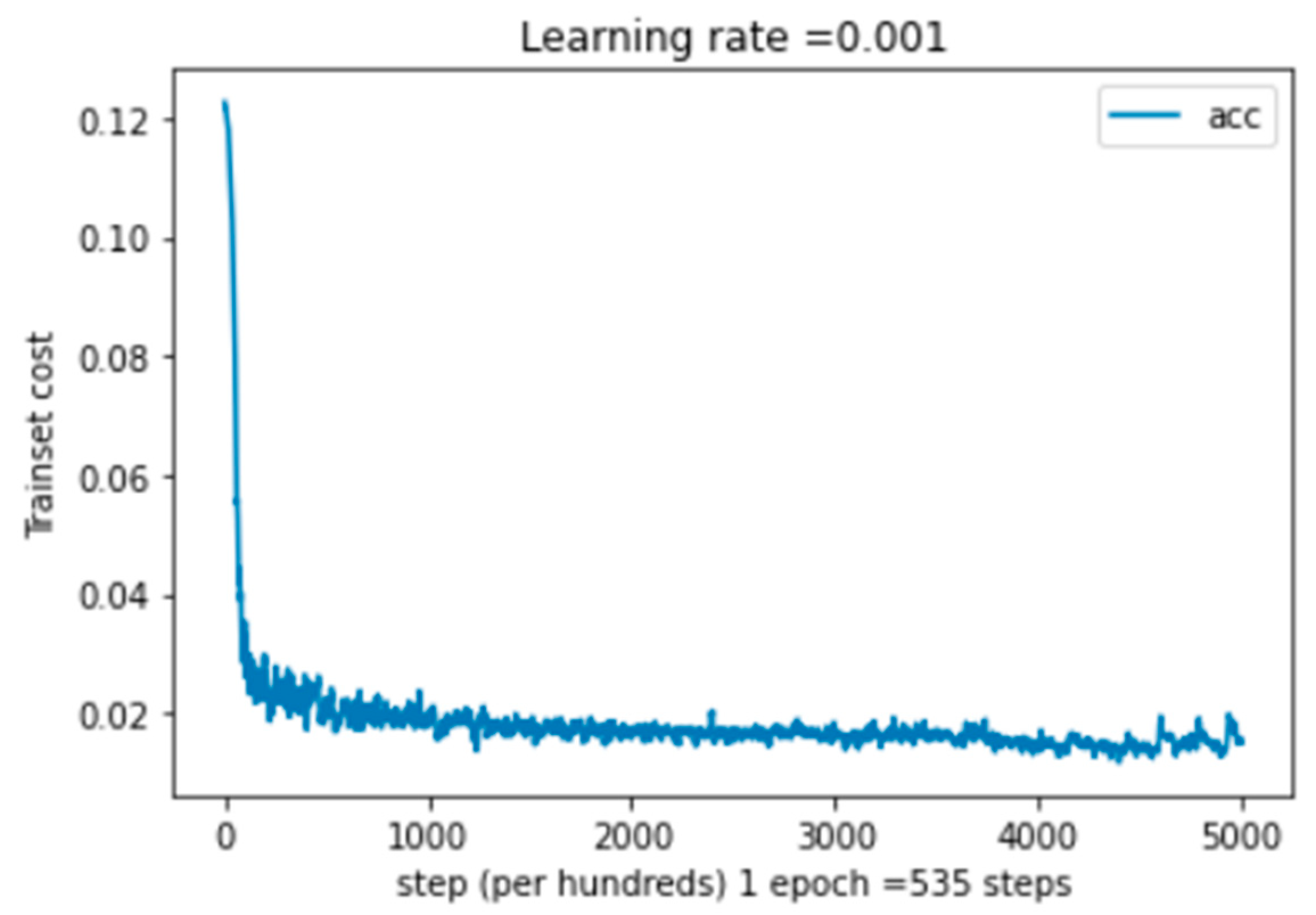
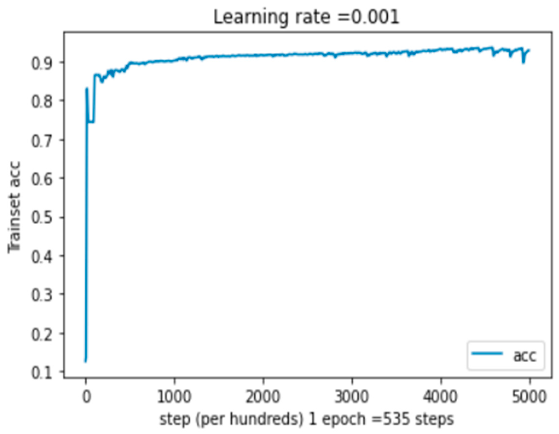
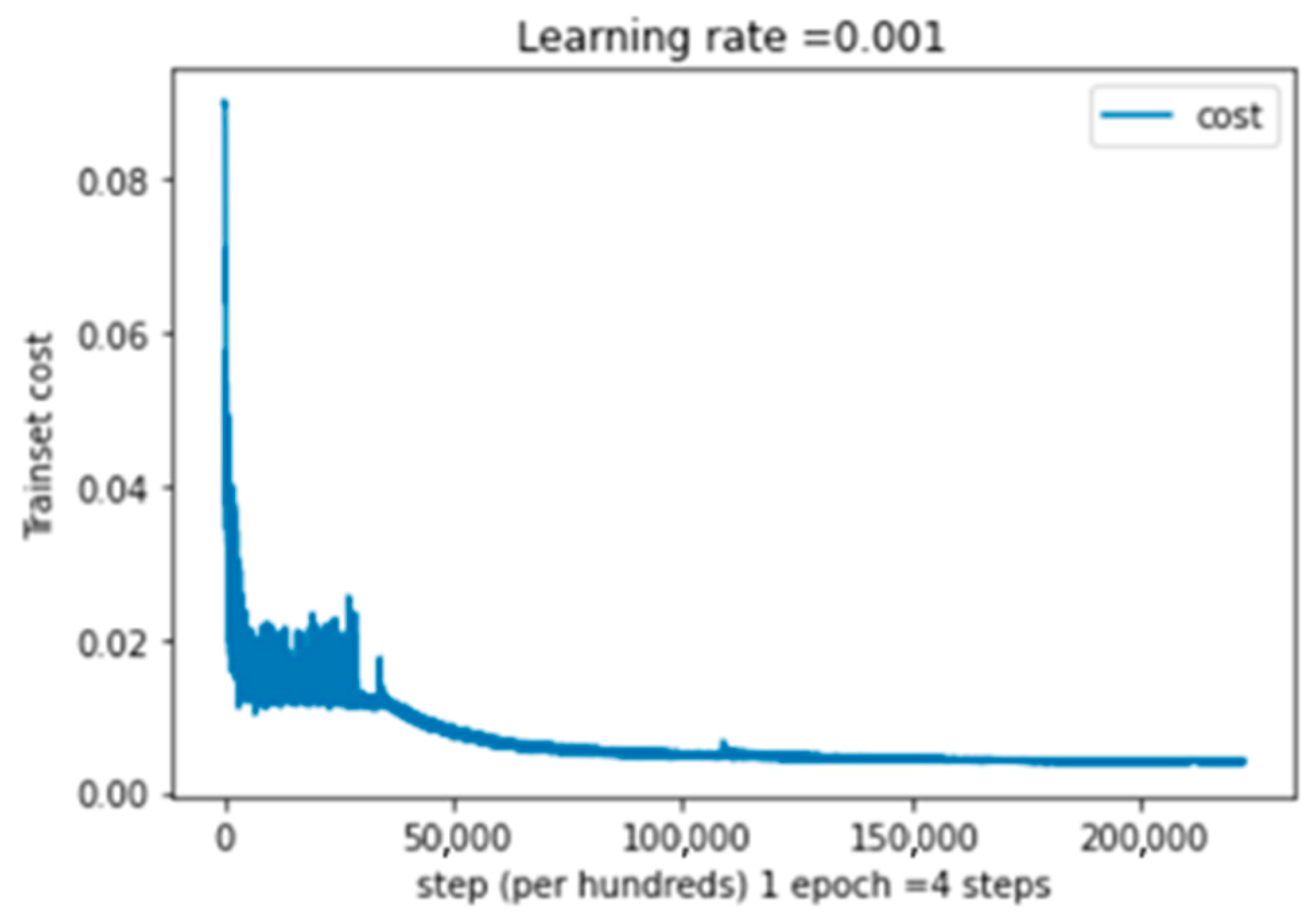
5.4. Performance Evaluation

We evaluated the performance of our system through the following steps: the first contains a detailed study of the multimodal system, the second presents a test on the one-modality system, and the third is a comparison with existing works.

5.4.1. Performance Study on Multimodal System

According to

Table 1. Classification report for the MELD dataset (multimodal system) based on precision, recall, and F1 score.

Class	Precision	Recall	F1-Score	Support
class 1	0.98	1	0.99	4710
class 2	1	1	1	25,470
class 3	0.87	0.94	0.9	268
class 4	0.95	0.94	0.95	684
class 5	0.99	0.95	0.97	1743
class 6	0.89	0.96	0.92	271
class 7	0.98	0.93	0.96	1108
Macro Avg	0.95	0.96	0.95	—
Weighted Avg	0.99	0.99	0.99	34,254

, we can see that our system produced effective results in terms of precision, recall, and F1 score, which is supported by the close values for the macro average and weighted average; on the other hand, the accuracy value is above 99%.

Table 2. Multimodal confusion matrix for MELD Dataset (7-class classification).

Predicted	0	1	2	3	4	5	6
Actual
0	4702	9	12	5	27	5	17
1	1	25,448	0	4	14	3	7
2	1	2	251	4	19	0	10
3	2	5	0	644	13	0	15
4	2	2	2	2	1650	0	10
5	0	4	2	10	10	259	16
6	2	0	2	4	10	4	1033

presents the multimodal confusion matrix for the MELD dataset, illustrating the classification performance across seven classes.

Table 1, Figure 5, and Figure 6 show, respectively, the classification report, the training cost, and the training accuracy for our multimodal system. We can observe that the cost curve’s greatest value is obtained at about 0 epochs and that it decreases as the number of epochs rises. The value is achieved at a cost of 0.0016. In terms of training accuracy, we observe that the maximum value is attained, followed by a drop to the maximum value, which stabilizes after a predetermined number of epochs. The value then rises to 99.22%. In the multimodal confusion matrix, the maximum value of the true label is 25,448 for class 1. This represents the high value in this matrix.

Table 3. Comparison of performance (MELD [15,16] dataset).

Models	Dataset	Parameters	Size (MB)	Accuracy (%)
DMCNN (our method)	MELD [15,16]	529,888	12.13	99.22
MNN [8,9]	MELD [15,16]	528,948	12.11	98.43

shows the evaluation of our approach, DMCNN, compared with MNN [8,9] in terms of accuracy concerning the MELD [15,16] datasets, depending on parameters (weight and bias) and module size in megabits (MB).

According to the results obtained, we note that the proposed approach achieves good performance criteria. Indeed, the results clearly demonstrate that the DMCNN model outperforms the MNN [8,9] model, achieving an accuracy of 99.22% compared to 98.43%.

5.4.2. Performance Results on Single Modality System

Above, we studied the multimodal system. In what follows, we continue with the single modality of the proposed method.

The classification report results shown in

Table 4. Classification report for the CIFAR-10 dataset (single modality system) based on precision, recall, and F1 score.

Class	Precision	Recall	F1-Score	Support
class 1	0.98	0.98	0.98	4027
class 2	0.99	0.99	0.99	4021
class 3	0.98	0.97	0.97	3970
class 4	0.97	0.97	0.97	4067
class 5	0.97	0.97	0.97	4067
class 6	0.96	0.97	0.96	3985
class 7	0.99	0.98	0.98	4004
class 8	0.97	0.98	0.97	3983
class 9	0.99	0.99	0.99	3983
class 10	0.98	0.99	0.99	3960
Macro Avg	0.98	0.98	0.98	—
Weighted Avg	0.98	0.98	0.98	40,000

demonstrate the effectiveness of our approach for the unimodal system in terms of precision, recall, and F1 score. Additionally, the accuracy rate reached 98%.

Table 5. Single modality confusion matrix for the CIFAR-10 dataset (10-class classification).

Predicted	0	1	2	3	4	5	6	7	8	9
Actual
0	3959	5	21	9	0	5	0	11	11	11
1	3	3983	1	2	0	1	0	3	5	5
2	10	0	3835	13	21	0	1	9	6	6
3	7	22	16	3962	25	0	16	0	1	6
4	8	27	27	8	3849	27	14	5	1	3
5	3	18	18	26	12	3983	9	1	1	4
6	6	12	4	1	31	9	3914	2	3	3
7	15	1	5	3	2	3	1	3917	2	3
8	12	6	5	4	1	3	3	5	3947	3
9	25	6	1	5	3	4	3	3	3	3914

presents the confusion matrix for the CIFAR-10 dataset [2], highlighting the model’s classification accuracy across all 10 classes.

The training cost of a single modality for the CIFAR-10 dataset [2] is shown in Figure 7 as a function of epochs, where one epoch equals four steps. As can be seen, the greatest value is attained at about zero epochs and decreases as the number of epochs rises. For the CIFAR-10 [2] dataset, the cost is 0.003 or less.

Regarding the training accuracy shown in Figure 8, we can see that for the latter, the maximum value is attained, followed by a fall and then a return to the maximum value. After a given number of epochs, this maximum value stabilizes at 97,81%. On the other hand, the unimodal system’s matrix of confusion (Table 5) shows that the maximum true etiquette value for class one is 3983. This stands for the highest value in this matrix.

Based on the provided dataset CIFAR-10 [2],

Table 6. Performance comparison of a single modal system applied to CIFAR-10 [2] dataset.

Models	Parameters	Size (MB)	Top 1 Accuracy (%)	Top 5 Accuracy (%)	GPU (GB)
DMCNN (ours)	12,960	0.30	97.78	98.58	4 (CPU)
MNN [8,9]	12,960	0.30	97.21	98.27	4 (CPU)
Vision Transformers
ViT [10]	624,970	213.15	77.06	98.46	13.9
ViP [19]	662,410	77.14	79.50	98.91	4.9
ViL [20]	506,186	69.69	63.17	96.13	2.3
ViN [17]	621,402	77.13	77.81	98.61	4.3
Compact Convolutional Transformers
CCT [18]	905,547	225.47	82.23	99.04	14.7
CCP [18]	907,083	101.48	82.48	99.06	4.3
CCL [18]	790,859	94.04	80.05	98.92	3.5
CCN [3]	906,075	101.48	83.36	99.07	4.2
Convolutional Vision Transformer
CvT [18]	1,099,78	173.21	79.93	99.02	12.8
CvP [18]	827,914	100.17	83.19	99.20	4.8
CvL [18]	711,690	92.73	72.58	97.81	2.6
CvN [18]	826,906	100.17	83.26	99.14	4.3

compares our method with the original MNN [8,9] method, vision transformers (ViT [10], ViP, VIN, and Vil), compact convolutional transformers (CCT, CCP, CCL, and CCN [3]) [17], and convolutional vision transformers (CvT, CvP, CvL, and CvN) [18]. The comparison is based on the weight and bias of the parameters, the module size in megabits (MB), the top 1 accuracy, the top 5 accuracy, and GPU in gigabits (GB).

We note that the DMCNN model obtained better results than any of the Xformer models concerning image classification. Table 6 shows that our method effectively outperforms even the original version of MNN [8,9] in the CIFAR-10 [2] dataset. All Xformer models use almost the same number of parameters as quadratic attention, while DMCNN uses a significantly low number of parameters in addition to a lower storage space among all Xformer models to achieve comparable performance. In addition to using fewer parameters, DMCNN ultimately achieved the top 1 and top 5 models’ best accuracy, which are represented by 97.78% and 98.58%, respectively, when compared to all other models mentioned.

5.5. Comparison with State-of-the-Art Methods

To evaluate the performance of our approach, we compared it with other state-of-the-art methods. We considered relevant approaches that have good accuracy for the Yale-B [21] and CK+ [22] datasets. We drew a comparison with the methods proposed by [1] and [8,9]. The obtained results are presented in

Table 7. A brief evaluation of our proposed approach in relation to similar studies in terms of accuracy.

Models	Dataset	Accuracy (%)
DMCNN	Yale-B	99.90
McDFR (2015) [1]	Yale-B	99.66
DMCNN	CK+	99.69
MNN (2021) [8,9]	CK+	98.65

.

Table 7 shows that our proposed method achieves higher accuracy, which matches the state-of-the-art performance and propounds the robustness in image classification.

6. Conclusions and Discussion

In this paper, the DMCNN model, whose architecture presents a shortcut that researchers can rely on to accurately classify data and extract informative features, is discussed. The formal method can, in fact, rely on either a singular or a multimodal approach. Typically, there are two basic steps: first, properly detecting and sorting the components, and second, fusing the extracted features to achieve the best possible result. Among all Xformer models, DMCNN was the most efficient. In this regard, this model is the most flexible, as it deals with data of different sizes without the need to unify their length, and it is the most accurate solution for the overfitting problem. Moreover, it is the most optimal when it comes to storage space and the accurate number of trainable parameters, not to mention its ability to work on multiple kinds of multimedia content, such as image, speech, text, signal, etc., Above all, not only theoretically but also experimentally, the DMCNN model is capable of separating the important features from the unimportant ones, subsequently corroborating the proportional relationship between the model’s accuracy and the number of components.

References

1. Chen, X. Learning Multi-channel Deep Feature Representations for Face Recognition. JMLR Workshop Conf. Proc. 2015, 44, 60–71. [Google Scholar]
2. Bengio, Y.; Courville, A.; Vincent, P. Representation learning: A review and new perspectives. IEEE Trans. Pattern Anal. Mach. Intell. 2013, 35, 1798–1828. [Google Scholar] [CrossRef] [PubMed]
3. Saxena, A. An Introduction to Convolutional Neural Networks. Int. J. Res. Appl. Sci. Eng. Technol. 2022, 10, 943–947. [Google Scholar] [CrossRef]
4. Sabour, S.; Hinton, G.E. Dynamic Routing Between Capsules. arXiv 2017, arXiv:1710.09829. [Google Scholar]
5. Sun, J.; Fard, A.P.; Mahoor, M.H. XnODR and XnIDR: Two Accurate and Fast Fully Connected Layers for Convolutional Neural Networks. arXiv 2021, arXiv:2111.10854. [Google Scholar] [CrossRef]
6. Jeevan, P.; Sethi, A. Vision Xformers: Efficient Attention for Image Classification. arXiv 2021, arXiv:2107.02239. [Google Scholar] [CrossRef]
7. Chen, T.; Zhang, Z.; Ouyang, X.; Liu, Z.; Shen, Z.; Wang, Z. “BNN - BN = ?”: Training binary neural networks without batch normalization. In Proceedings of the 2021 IEEE/CVF Conference on Computer Vision and Pattern Recognition Workshops (CVPRW), Nashville, TN, USA, 19–25 June 2021; pp. 4614–4624. [Google Scholar] [CrossRef]
8. Filali, H.; Riffi, J.; Aboussaleh, I.; Mahraz, A.M.; Tairi, H. Meaningful Learning for Deep Facial Emotional Features. Neural Process. Lett. 2021, 54, 387–404. [Google Scholar] [CrossRef]
9. Filali, H.; Riffi, J.; Boulealam, C.; Mahraz, M.A.; Tairi, H. Multimodal Emotional Classification Based on Meaningful Learning. Big Data Cogn. Comput. 2022, 6, 95. [Google Scholar] [CrossRef]
10. Dosovitskiy, A.; Beyer, L.; Kolesnikov, A.; Weissenborn, D.; Zhai, X.; Unterthiner, T.; Dehghani, M.; Minderer, M.; Heigold, G.; Gelly, S. An image is worth 16x16 words: Transformers for image recognition at scale. arXiv 2020, arXiv:2010.11929. [Google Scholar]
11. Zhang, Z.; Zhang, H.; Zhao, L.; Chen, T.; Pfister, T. Aggregating Nested Transformers. arXiv 2021, arXiv:2105.12723. [Google Scholar] [CrossRef]
12. Deng, W.; Feng, Q.; Gao, L.; Liang, F.; Lin, G. Non-convex learning via replica exchange stochastic gradient MCMC. In Proceedings of the 37 th International Conference on Machine Learning, Online, 13–18 July 2020; pp. 2452–2461. [Google Scholar]
13. Yun, S.; Han, D.; Chun, S.; Oh, S.J.; Choe, J.; Yoo, Y. CutMix: Regularization strategy to train strong classifiers with localizable features. In Proceedings of the 2019 IEEE/CVF International Conference on Computer Vision (ICCV), Seoul, Republic of Korea, 27 October–2 November 2019; Volume 2019, pp. 6022–6031. [Google Scholar] [CrossRef]
14. Lu, Z.; Member, S.; Sreekumar, G.; Goodman, E.; Banzhaf, W.; Deb, K.; Boddeti, V.N. Neural Architecture Transfer. arXiv 2020, arXiv:2005.05859. [Google Scholar] [CrossRef] [PubMed]
15. Poria, S.; Hazarika, D.; Majumder, N.; Naik, G.; Cambria, E.; Mihalcea, R. Meld: A multimodal multi-party dataset for emotion recognition in conversations. arXiv 2018, arXiv:1810.02508. [Google Scholar]
16. Chen, S.-Y.; Hsu, C.-C.; Kuo, C.-C.; Ku, L.-W. Emotionlines: An emotion corpus of multi-party conversations. arXiv 2018, arXiv:1802.08379. [Google Scholar]
17. Xiong, Y.; Zeng, Z.; Chakraborty, R.; Tan, M.; Fung, G.; Li, Y.; Singh, V. Nyströmformer: A nyström-based algorithm for approximating self-attention. In Proceedings of the AAAI Conference on Artificial Intelligence, Virtual, 2–9 February 2021; Volume 35, pp. 14138–14148. [Google Scholar]
18. Wu, H.; Xiao, B.; Codella, N.; Liu, M.; Dai, X.; Yuan, L.; Zhang, L. Cvt: Introducing convolutions to vision transformers. In Proceedings of the IEEE/CVF International Conference on Computer Vision, Montreal, BC, Canada, 11–17 October 2021; pp. 22–31. [Google Scholar]
19. Li, J.; Zhang, H.; Xie, C. ViP: Unified Certified Detection and Recovery for Patch Attack with Vision Transformers. In Proceedings of the European Conference on Computer Vision, Tel Aviv, Israel, 23–27 October 2022; Springer: Cham, Switzerland, 2022; pp. 573–587. [Google Scholar]
20. Kim, W.; Son, B.; Kim, I. Vilt: Vision-and-language transformer without convolution or region supervision. In Proceedings of the International Conference on Machine Learning, PMLR, Virtual, 18–24 July 2021; pp. 5583–5594. [Google Scholar]
21. Fedorov, I.; Giri, R.; Rao, B.D.; Nguyen, T.Q. Robust Bayesian method for simultaneous block sparse signal recovery with applications to face recognition Proc. Int. Conf. Image Process. 2016, 2016, 3872–3876. [Google Scholar] [CrossRef]
22. Lucey, P.; Cohn, J.F.; Kanade, T.; Saragih, J.; Ambadar, Z.; Matthews, I. The extended cohn-kanade dataset (ck+): A complete dataset for action unit and emotion-specified expression. In Proceedings of the 2010 IEEE Computer Society Conference on Computer Vision and Pattern Recognition-Workshops, San Francisco, CA, USA, 13–18 June 2010; IEEE: Piscataway, NJ, USA, 2010; pp. 94–101. [Google Scholar]
Figure 1. A generalized meaningful neural network architecture.
Computation 13 00093 g001
Figure 2. Calculate vector output layer.
Computation 13 00093 g002
Figure 3. The DMCNN proposed for classification.
Computation 13 00093 g003
Figure 4. Calculation weight of each component in DMCNNA.
Computation 13 00093 g004
Figure 5. Training cost as a function of epochs for the MELD [15,16] dataset, where 1 epoch = 535 steps.
Computation 13 00093 g005
Figure 6. Training accuracy as a function of epochs for the MELD [15,16] dataset, where 1 epoch = 535 steps.
Computation 13 00093 g006
Figure 7. Training cost as a function of epochs for the CIFAR-10 [2] dataset, where 1 epoch = 4 steps.
Computation 13 00093 g007
Figure 8. Training accuracy as a function of epochs for the CIFAR-10 [2] dataset, where 1 epoch = 4 steps.
Computation 13 00093 g008