Abstract
Accurate fault diagnosis in analog circuits faces significant challenges owing to the inherent complexity of fault data patterns and the limited feature representation capabilities of conventional methodologies. Addressing the limitations of current convolutional neural networks (CNN) in handling heterogeneous fault characteristics, this study presents an efficient channel attention-enhanced multi-input CNN framework (ECA-MI-CNN) with dual-domain feature fusion, demonstrating three key innovations. First, the proposed framework addresses multi-domain feature extraction through parallel CNN branches specifically designed for processing time-domain and frequency-domain features, effectively preserving their distinct characteristic information. Second, the incorporation of an efficient channel attention (ECA) module between convolutional layers enables adaptive feature response recalibration, significantly enhancing discriminative feature learning while maintaining computational efficiency. Third, a hierarchical fusion strategy systematically integrates time-frequency domain features through concatenation and fully connected layer transformations prior to classification. Comprehensive simulation experiments conducted on Butterworth low-pass filters and two-stage quad op-amp dual second-order low-pass filters demonstrate the framework’s superior diagnostic capabilities. Real-world validation on Butterworth low-pass filters further reveals substantial performance advantages over existing methods, establishing an effective solution for complex fault pattern recognition in electronic systems.
1. Introduction
Currently, analog circuit has become an important pillar in military, national defense, aviation and other fields. Therefore, accurate and efficient fault diagnosis of analog circuits has become a research hotspot in the field of circuit testing [1,2,3]. According to statistical data, electronic circuits are developing in the direction of high integration and high complexity, in which the fault rate of analog circuits is more than 80%, which easily leads to frequent accidents, financial losses, and even casualties [4,5,6]. Hence, analog circuit fault diagnosis technology is regarded as a key technology in ensuring the normal operation of electronic equipment. Early and accurate diagnosis of analog circuit faults can help further predict the fault time of the analog circuit, calculate the residual effective performance of the circuit, reduce the fault rate of the analog circuit and improve its operational efficiency. Thus, developing an effective and fast electronic circuit diagnosis strategy has become an urgent need in the field of analog circuit fault diagnosis [7].
Early analog circuit fault diagnosis relied on the fault dictionary model, which matches faults by pre-storing fault patterns. This approach enables fast matching and reduces computational costs in small-scale circuits or scenarios with limited fault patterns. However, as circuit complexity increases, traditional methods face challenges: they rely on a complete fault dictionary, which is costly to construct, and their accuracy declines under noise or environmental interference, limiting their applicability in complex circuit diagnosis. Li et al. [8] proposed a novel joint peak-to-peak analysis and worm analysis threshold method to address fault detection in locally nonlinear fuzzy autonomous ground vehicle systems with disturbances by establishing a set membership estimation. Ding et al. [9] studied the dynamic response of the Hodgkin–Huxley neuron model under periodic excitation. By using a phase return map, they converted the neuron firing signals into a 1D mapping and quantified the differences between chaotic and periodic states through symbolic dynamics, demonstrating the method’s applicability in transient signal analysis of power electronic device faults.
These studies show that with the continuous development of fault diagnosis technology, more and more innovative methods have been proposed and applied in different fields. Meanwhile, with the rapid development of the semiconductor industry, the demand for more advanced circuit fault diagnosis techniques has become increasingly urgent. To address this, data-driven knowledge-based methods were introduced to solve the inefficiency of traditional fault diagnosis. Wang et al. [10] proposed an improved spiking neural network (ISNN) for intershaft bearing fault diagnosis. They developed an encoding method to convert raw vibration data into spike sequences and validated its accuracy and effectiveness. To quickly learn and adapt to time-series tasks, Wang et al. [11] developed an improved echo state network (IESN) for fault diagnosis of tractor power shift systems. By simulating 30,000 sets of test data and using an enhanced dynamic time warping algorithm for data segmentation, the improved ESN was used to classify fault samples. The results show that the improved ESN outperforms traditional algorithms in both training speed and accuracy. After neural networks achieved high diagnostic accuracy, research on fault diagnosis based on machine learning methods became a popular research area [12].
Binu et al. [13] designed a Ride NN classifier using a rider optimization algorithm to optimize neural network (NN); Zhang et al. [14] proposed a fault diagnosis method based on unsupervised clustering to improve support vector machine (SVM). Although machine learning has achieved high performance in fault diagnosis, two major drawbacks still limit its development: (1) the hyperparameters in classification models are mostly set empirically, making the diagnosis results highly influenced by human factors; (2) shallow learning models are not suitable for large-scale data environments and tend to overlook potential features. In recent years, deep learning methods have been widely applied in fault diagnosis [15,16,17] due to their powerful data feature extraction capabilities and excellent ability [18] to describe nonlinear fault dynamics [19].
Among deep learning methods, deep belief networks (DBNs) have proven effective in multi-layer unsupervised learning and supervised fine-tuning. By extracting key features of data through multiple nonlinear transformations, DBNs can be applied to fault diagnosis [20,21,22]. Chen et al. [23] proposed a DBN-based fault diagnosis method for analog circuits, which can adaptively extract features from time-series signals and automatically classify faults. However, DBNs have limitations in handling complex fault patterns and optimal classification within the same category. The lack of refined classification may affect the overall model performance, particularly in dynamic and diverse fault scenarios. To address this issue, Su et al. [24] used a DBN to extract deep features from the output signal of analog circuits and optimized the support vector machine (SVM) using gray wolf optimization (GWO), resulting in the GWO-SVM model for diagnostic classification. Experimental results show that this method significantly improves diagnostic accuracy and shortens diagnosis time. However, DBNs still struggle with the 2D image structure and perform poorly when handling large high-dimensional datasets. As a result, researchers have begun to explore alternative deep-learning architectures. For example, Lee et al. [25] proposed a convolutional deep belief network (CDBN), which effectively addresses the challenges of high-dimensional images and can scale these images effectively. However, when large datasets are involved, the CDBN model tends to overfit. To solve this issue, Goodfellow et al. [26] introduced generative adversarial network (GAN), which can alleviate the overfitting problem and reduce the reliance on large datasets [27]. He et al. [28] proposed to use the cross wavelet transform (XWT) to capture features, regularize and construct three-channel feature image data, build a model with convolutional neural network (CNN), and extend GAN into a supervised classifier. Experiments show that GAN can alleviate over-fitting and reveal the nonlinear relationship between fault source and fault feature, and has a good application prospect in analog circuit fault diagnosis. However, GAN requires a longer training time, and the quality of the generated samples is also difficult to control. Therefore, it still faces challenges in stability and optimization, especially in real-world environments with noisy or incomplete data. Despite the potential of DBN and GAN, they still fall short of fully addressing the complexity and accuracy requirements of analog circuit diagnosis.
To fully leverage the temporal correlation features of analog circuit signals, enhance the model’s ability to mine data, and improve fault classification accuracy, CNN has gradually become a key focus in the research of analog circuit fault diagnosis due to their powerful feature extraction capabilities. Kim et al. [29] found that CNN has enough acceptance ability in the frequency domain and time domain, but it has poor generalization ability in the time domain and high acceptance ability in the complex frequency domain, and thus it is concluded that the choice of working domain is related to the network model. Du et al. [30] suggested to use CNN to carry out analog circuit fault diagnosis. The experimental results of Sallen-Key filter circuit show that CNN can effectively simplify the fault diagnosis process and improve the fault diagnosis rate. Zhang et al. [31] proposed a new analog circuit soft fault diagnosis method, which combines the backward difference strategy with CNN and the global average pooling (GAP), the former performs data processing, while the latter carries out fault diagnosis and classification. Experimental results show that this method has good applicability in the field of analog circuit fault diagnosis. However, the importance of the information in each channel is different in practice, while the traditional CNN defaults to the equal importance of each channel’s information and lacks the screening of important features. Therefore, squeezed excitation networks (SENet) and selective kernel networks (SKNet) are proposed to optimize CNNs in terms of dimensionality and convolutional kernels [32,33]. The theory suggests that while networks with deeper structures may obtain higher performance, they are also more prone to gradient disappearance or explosion, leading to slow convergence and over-fitting problems [34]. Therefore, He et al. [35] proposed a deep residual network (ResNet) structure, which addresses the problem of performance degradation due to increasing network depth, resulting in a higher performance of the whole network. Considering the long training time and low unsupervised learning accuracy of residual networks, from the perspective of improving the training speed and accuracy, Zhou et al. [36] improved the structure of ResNet by combining SE-Net and multi-level depth feature fusion. Tong et al. [37] embedded a multi-scale deep separable expression recognition network based on convolutional block attention module (CBAM) in the residual network to improve the weight of important features in the network, eliminate irrelevant redundant features and enhance the robustness of the network. Tang et al. [38] utilized multi-input convolution to combine time domain and frequency domain to accurately extract features, and the experimental results show that the proposed model can improve the recognition rate and convergence performance of the traditional convolution model, and has good robustness and generalization ability.
Most of the above literature only studies the problem of analog circuit fault from the perspective of time domain or frequency domain, while deep learning has some problems in fault diagnosis, such as complex models and difficulty in extracting essential features. In order to comprehensively capture the time domain feature information and frequency domain feature information, the multiple-convolutional neural network (MI-CNN) model is considered as the basic framework for the extraction of the special whole. Meanwhile, in order to improve the performance degradation of deep learning due to the deepening of network structure, the ECA module is used to optimize the model. Therefore, a model based on ECA-MI-CNN is constructed in this paper. Based on single-input CNN, the proposed model uses MI-CNN to realize information fusion, and ECA module is added in the feature extraction process to reduce the computation on the premise of ensuring network performance. Taking the fault diagnosis of Butter-worth low-pass filter and two-stage quad op-amp dual second-order low-pass filter as examples, the comprehensive performance of the ECA-MI-CNN model is verified by several comparison experiments.
2. ECA-MI-CNN
2.1. Traditional CNN and BN Layer
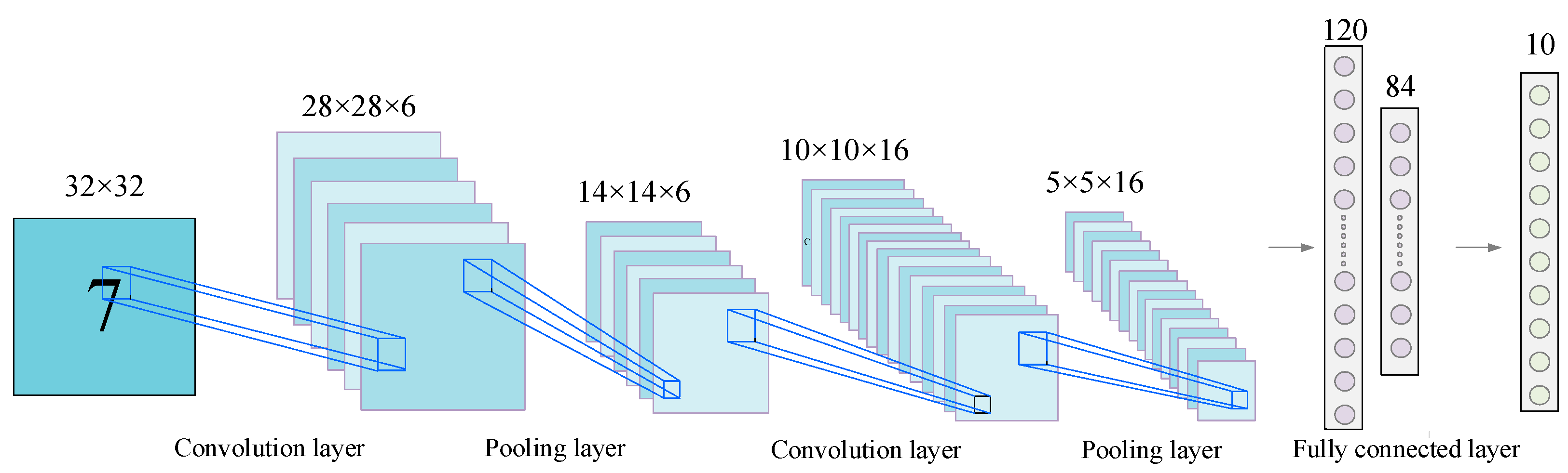
CNNs are outstanding in the field of image data with the advantage of convolutional operations, and the typical structure is shown in Figure 1.
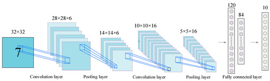
Figure 1.
Typical Structure of CNN.
The convolution layer is a convolutional operation to extract features from the information in the perceptual field by means of a designed convolutional kernel, as shown in (1):
where is the number of layers at the time of model building, is the activation function chosen, is the k-th feature mapping of the l-1th layer, is the individual convolution kernel, and is the bias.
CNN can extract features efficiently. In addition, the local connectivity and shared weights used by CNN reduce the complexity of deep networks, and on the other hand reduce the risk of overfitting. However, deep neural networks suffer from difficulties in training and slow convergence as the network depth deepens. The addition of a batch normalization (BN) layer after the convolutional layer can effectively improve the problem.
The conduction process of the BN layer is as follows:
- (1)
- Calculation of sample average.
- (2)
- Calculation of sample variance.
- (3)
- Standardization of sample data.
- (4)
- Perform translation and scaling processing.
2.2. MI-CNN
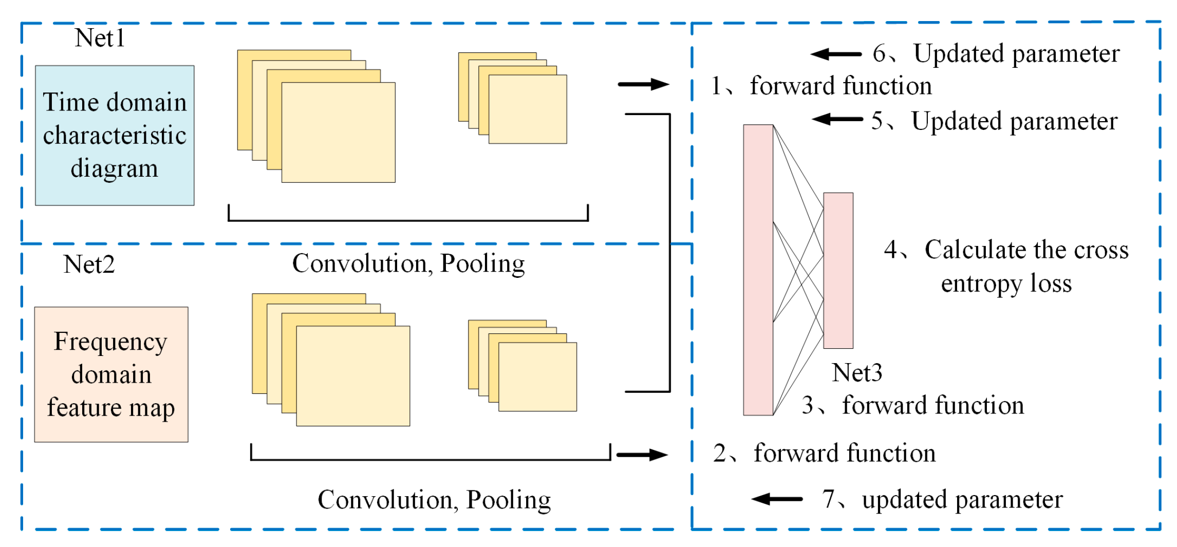
The advantage of the MI-CNN feature fusion framework is that it matches different convolutional and pooling strategies for different features, fully utilizing the feature extraction capability of the convolutional neural network, and finally fusing and feeding the higher-order features to the Softmax layer to select and non-linearly fit the extracted higher-order features, greatly improving the classification performance of the network. The process of the MI-CNN structure is shown in Figure 2:
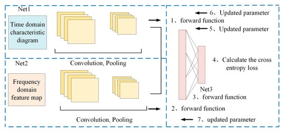
Figure 2.
Typical structure of MI-CNN.
- (1)
- Input Stage: The input images are fed into two independent subnetworks, Net1 and Net2, for feature extraction.
- (2)
- Feature Extraction: Net1 and Net2 employ different convolution and pooling strategies to extract features at various levels and forward the information.
- (3)
- Feature Fusion: The extracted features from Net1 and Net2 are fused in the fully connected layer of Net3 to effectively integrate the information from different networks.
- (4)
- Classification Calculation: The fused high-order features are passed to the Softmax layer for classification, and the cross-entropy loss is computed.
- (5)
- Backpropagation: The computed loss is propagated backward to optimize the weights and biases in Net3.
- (6)
- Parameter Update: The parameters in Net1 and Net2 are updated to enhance feature extraction capability and improve the overall classification performance of the network. Net1 and Net2 are, respectively, used for operations such as convolution and information forwarding.
2.3. ECA Module
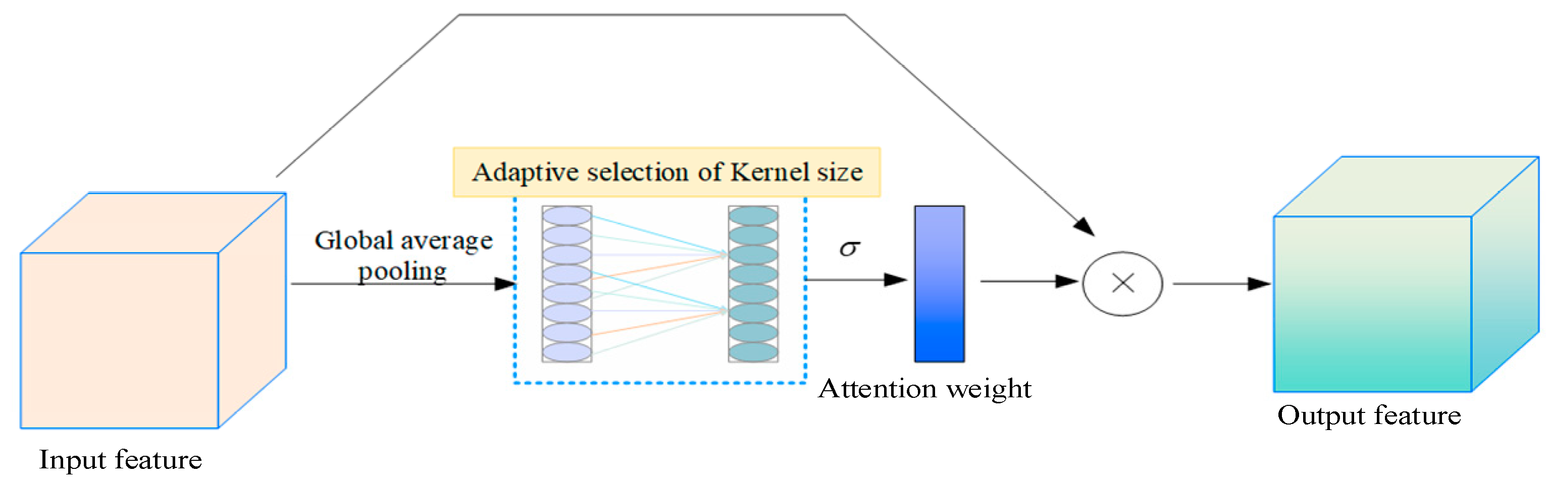
In recent years, studies have demonstrated that channel attention has significant potential to enhance CNN performance. To achieve better model results, channel attention modules have evolved towards greater complexity, leading to increased computational parameters and longer training times. Compared with the more complex SE module, the ECA module removes the intermediate fully connected layer and instead adopts a local cross-channel interaction mechanism, considering only the interactions between each channel and its k nearest neighbors. This design effectively reduces the number of parameters and shortens training time while maintaining competitive performance.
The structure of the ECA module, as illustrated in Figure 3, consists of three main steps:
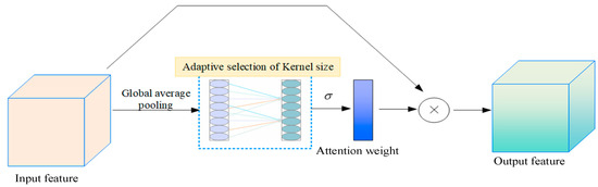
Figure 3.
ECA structure.
Global Average Pooling (GAP): The input feature map undergoes GAP to generate a channel-wise descriptor, summarizing global spatial information.
One-Dimensional Convolution with Adaptive Kernel Size: Instead of a fully connected layer, a 1D convolution operation with an adaptive kernel size is applied to model cross-channel dependencies. The kernel size k is adaptively determined based on the number of input channels, ensuring efficient feature interactions.
Channel Reweighting: The output of the 1D convolution is processed using a sigmoid activation function to generate attention weights, which are then multiplied element-wise with the original feature map to enhance informative channels and suppress less relevant ones.
The ECA module works by first applying GAP to the data of each channel after the convolutional transform, in order to obtain the global information of each channel and to compensate for the inability to obtain information outside the local sensory field of view due to the small convolutional kernel. The equation is as follows:
where is the feature channel, is the global eigenvalue of , c is the number of feature channels, and W and H represent the width and length of the data. Because the purpose of ECA is local cross-channel interaction, only the interaction with k adjacent channels is considered in the calculation of channel weights, and the equation is as follows:
where represents the set of k adjacent channels of , and represents the Sigmoid activation function. This local constraint avoids the interaction of the fully connected layer across all channels and greatly improves the efficiency of the model. In this way, the number of parameters involved in each ECA module is only k ∙ c, which is much less than the c2∙(c/r) parameters in the SE module. The expression can then be implemented by a one-dimensional convolution operation with k convolution kernels, with Equation (7):
k is a key parameter in the model, determining the size of the range of channel interactions, so the choice of k value is a key factor in the performance of the model. It has been experimentally verified that the value of k is related to the number of channels c. There is some mapping relationship between the two, and exponential functions are often applied to deal with this non-linear mapping relationship. Since the number of channels c is often set to an integer power of 2, the expression can be obtained as follows:
When the number of channels C is known, k can be obtained as:
where , b are the regulation parameters, which are 2 and 1, respectively.
2.4. ECA-MI-CNN Model
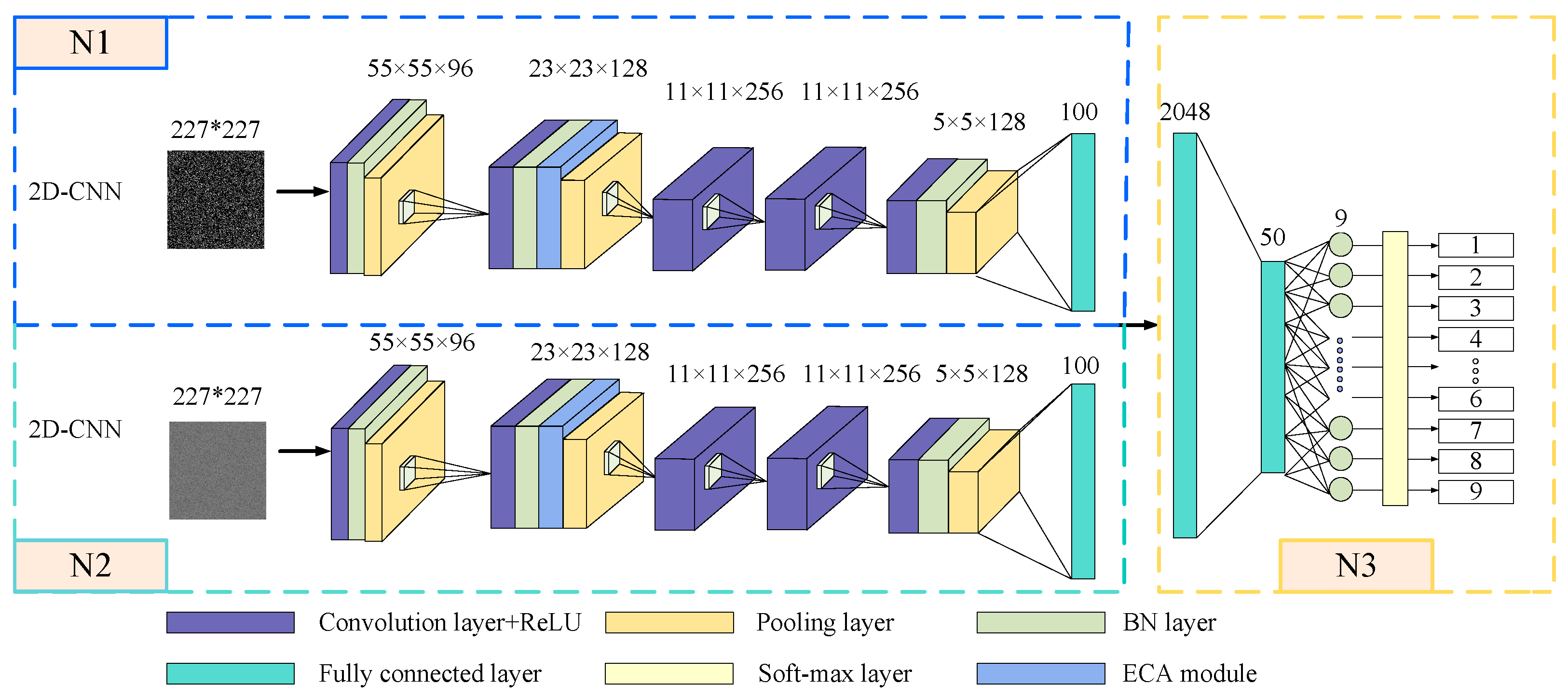
The structure of the ECA-MI-CNN model, shown in Figure 4, consists of N1, N2 and N3. The ECA-MI-CNN consists of two input layers, a convolutional layer, a modified linear unit (Rectified linear unit, ReLU), a BN layer, an ECA, a pooling layer, and a fully connected layer. the N1 and N2 layers consist of the convolutional layer + ReLU, a BN layer, an ECA module, and a pooling layer. In addition, in order to avoid the impact of convolutional kernel size on model performance in CNN, the kernel size and step size parameters of each convolutional layer in N1 and N2 are equal. The initial weights in the network are randomly generated, while the later weight parameters are obtained by the model continuously adjusted according to the number of iterations.
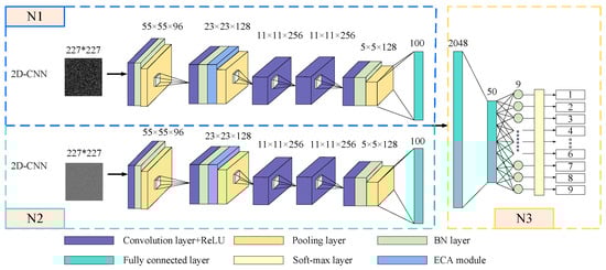
Figure 4.
ECA-MI-CNN model.
The convolutional layer with powerful feature extraction is used to extract features from the input information. The ReLU function speeds up operations and preserves the effects of the convolutional layer. The BN layer is used to increase the training speed and reduce the risk of overfitting during network training. The ECA simplifies the complexity of the model, simplifies computation, and improves model performance. The pooling layer is used to reduce the size of the matrix, reduce the number of parameters, and optimize the workload. N3 uses a fully connected layer (FC) to splice the time domain feature information from the N1 network and the frequency domain feature information from the N2 network to achieve comprehensive and accurate feature information extraction; the fully connected layer is applied to reduce the impact of feature location on classification, and finally, the output values are fed into the classifier for classification with a cross-entropy loss function.
3. Analog Circuit Fault Diagnosis Based on ECA-MI-CNN
3.1. Experimental Subjects
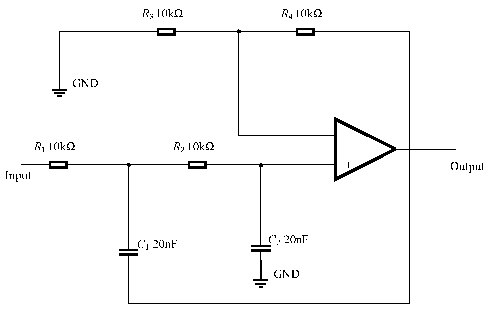
Under the influence of complex external environmental conditions, such as noise, temperature, and humidity, the parameters of circuit components may exceed their tolerance range, leading to performance degradation or even failure. To address this issue, this study selects the Butterworth low-pass filter (Figure 5) and the two-stage quad op-amp dual second-order low-pass filter (Figure 6) as research subjects. These two types of filters are widely used in practical engineering applications and hold significant theoretical and practical value. The Butterworth low-pass filter is particularly advantageous in scenarios requiring high filtering accuracy due to its flat passband response. In contrast, a two-stage quad op-amp dual second-order low-pass filter can simulate more complex filtering behaviors and offers higher tunability, making it suitable for circuit applications with stringent performance requirements. Furthermore, these filters effectively reflect common fault patterns in circuits, and their design and analysis methods serve as valuable references in fault detection research.
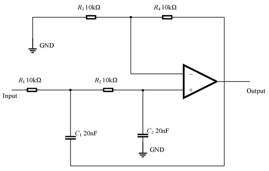
Figure 5.
Butterworth low-pass filter.
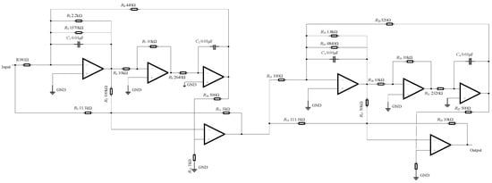
Figure 6.
Two-stage quad op-amp dual second-order low-pass filter.
In this study, we simulate deviations of components such as capacitors and resistors under major faults, minor faults, and normal conditions to analyze their impact on circuit performance. Using the obtained simulation dataset, we verify the effectiveness of the ECA-MI-CNN diagnostic model. Additionally, we construct a Butterworth experimental circuit and collect operational data under fault conditions to further evaluate the fault detection capability of the ECA-MI-CNN diagnostic model in an experimental environment.
3.2. Fault Data Acquisition and Processing
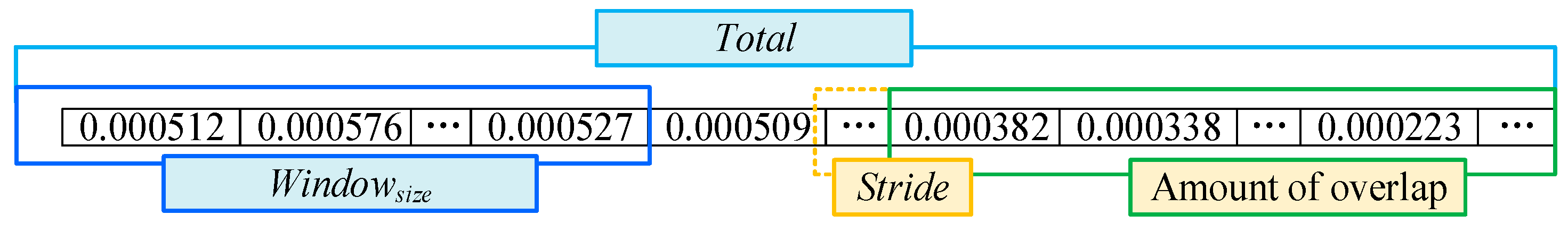
When building the model verification circuit, a 1 V, 1 kHz sinusoidal signal is applied to collect fault data. Due to the high demand for fault data, overlap sampling is utilized for data enhancement. The time information is a non-negligible factor and needs to be strictly matched to the time information when sampling, so the data is overlapped and sampled under the same time period.
where represents the total number of sampling points, represents the window size, represents the step size, and represents the total number of samples.
The overlap sampling method is shown in Figure 7, where 160,000 data points are sampled for different faults, each with a sample length of 51,529 and an offset of 1064, creating 100 fault samples. The samples are normalized and decomposed into 227 × 227 greyscale images. Labels are added to each type of fault to input the first self-network N1; the image data obtained are Fourier-transformed using image processing, and the resulting frequency domain information map is used as input data for the N2 network.
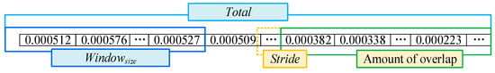
Figure 7.
Schematic diagram of an overlapping sampling method.
Figure 7 is a schematic diagram of overlapping sampling. A total of 160,000 data points were sampled for each different class of faults, and the length of each sample was 51,529 with an offset of 1064. According to the calculation of Equation (11), it is known that 100 227 × 227 time-domain feature maps (227 × 227 × 1 × 100) can be formed for each class of faults, and the time-domain feature maps were grayed out. The grayed-out time-domain feature maps are coded and processed (shown in Table 1) and input to sub-network N1; at the same time, the feature maps are processed by image Fourier transform to obtain the frequency domain feature maps, which are also processed by coding and input to sub-network N2.

Table 1.
Fault modes of Butterworth low-pass filter circuit.
3.3. Experimental Process
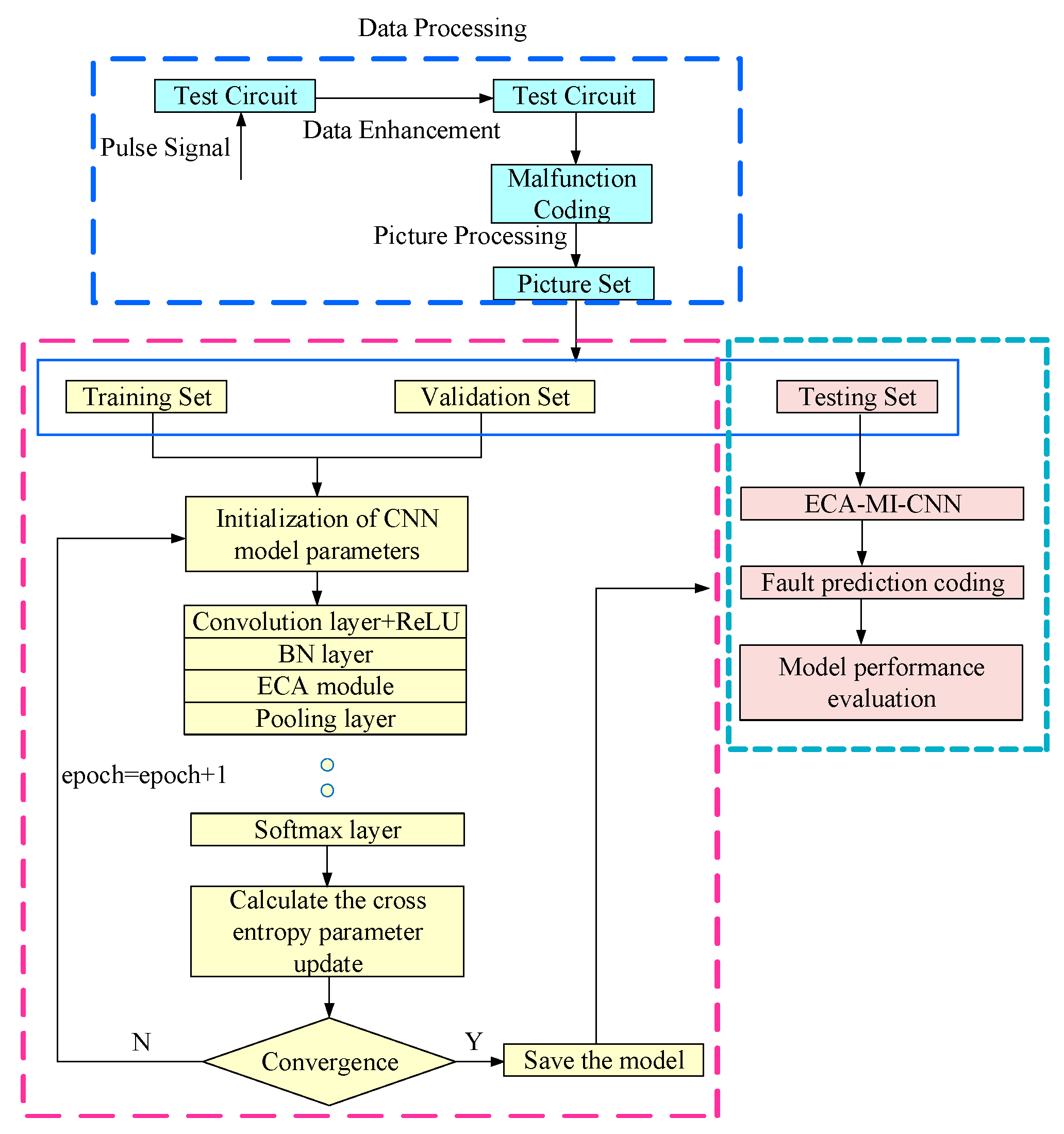
Figure 8 shows the ECA-MI-CNN model diagnosis process. In the model validation process, the fault data are first collected and coded for different fault types, and then the sample data are preprocessed to do some analysis and classification. Finally, the ECA-MI-CNN model proposed in this paper is established, and the superiority of the model is verified by experiments in the following process:
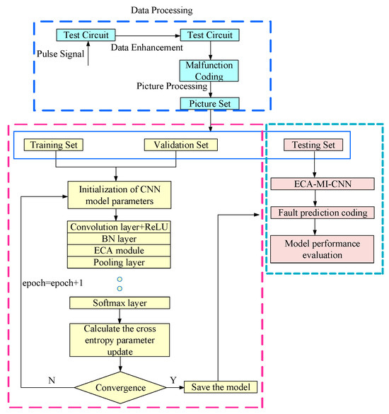
Figure 8.
ECA-MI-CNN model diagnosis process.
- (1)
- Collecting fault data after applying pulse signals to the circuit;
- (2)
- Performing overlapping sampling operations on the sample data to obtain the input time-domain feature maps of sub-network N1, while using the image Fourier transform technique to obtain the input frequency-domain feature maps of sub-network N2;
- (3)
- The 9 fault types obtained with the Butterworth low-pass filter are coded with “F1-F9”, and the 13 fault types obtained with the two-stage quad-operator dual second-order low-pass filter are coded with “F1–F13”. The 13 fault types obtained from the experimental object of the secondary four-operator dual second-order low-pass filter are coded with “F1–F13”.
- (4)
- The time domain feature set and frequency domain feature set are divided into training set (60%), validation set (20%), and test set (20%).
- (5)
- The ECA-MI-CNN model is built, and the cross-entropy loss function is used as the target condition to continuously adjust the network model to make the model optimal.
- (6)
- Compare the actual codes in the test set with the predicted codes generated by the model, and determine the correct classification result if the results are consistent, and determine the wrong classification if the results are inconsistent.
- (7)
- The comprehensive performance of the model is analyzed with different parameters.
3.4. Diagnosis Results of Butterworth Low-Pass Filter Circuit
Diagnostic experiments were carried out for resistor and capacitor faults in a Butter worth low-pass filter with a center frequency of 20 kHz.
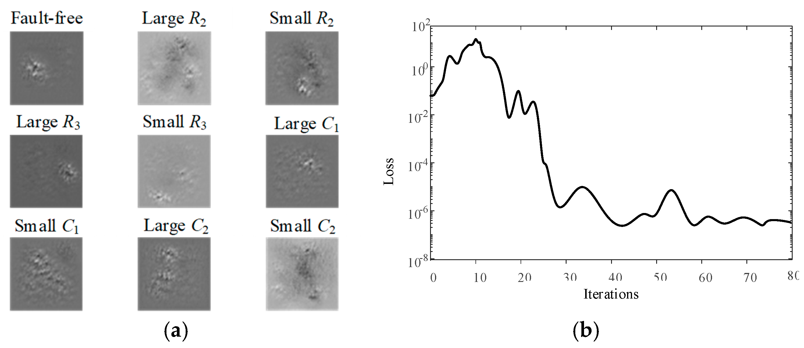
Table 1 shows the Butterworth low-pass filter circuit fault modes, which are set to the three cases of large, small and normal. When the resistor tolerance in the Butterworth low-pass filter exceeds 5% of the set tolerance and the capacitor size exceeds 10% of the tolerance, the resistor and capacitor are faulty and the fault type is marked as large, and when the resistor or capacitor is less than 5% or 10% of the tolerance, the fault occurs and the fault type is marked as small. When the resistance or capacitance does not exceed the set tolerance, no fault is judged to have occurred. Four components, R2, R3, and capacitors C1 and C2, were used as experimental objects for model verification through sensitivity testing. Figure 9a shows the characteristics of the fault signal of each device in the Butterworth low-pass filter, it can be seen that there is a clear difference between the nine fault characteristics and Figure 9b shows the loss function of the Butterworth low-pass filter versus the number of iterations, it can be obtained that the basic model stabilizes after 30 iterations and the loss value is stable between 10−8 and 10−6.
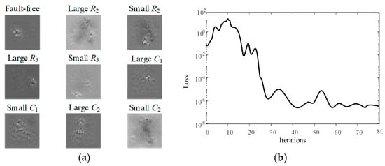
Figure 9.
Butterworth low pass filter fault signal feature diagram and loss function diagram: (a) Butterworth low-pass filter fault signal feature diagram; (b) relationship diagram of iteration times and loss function.
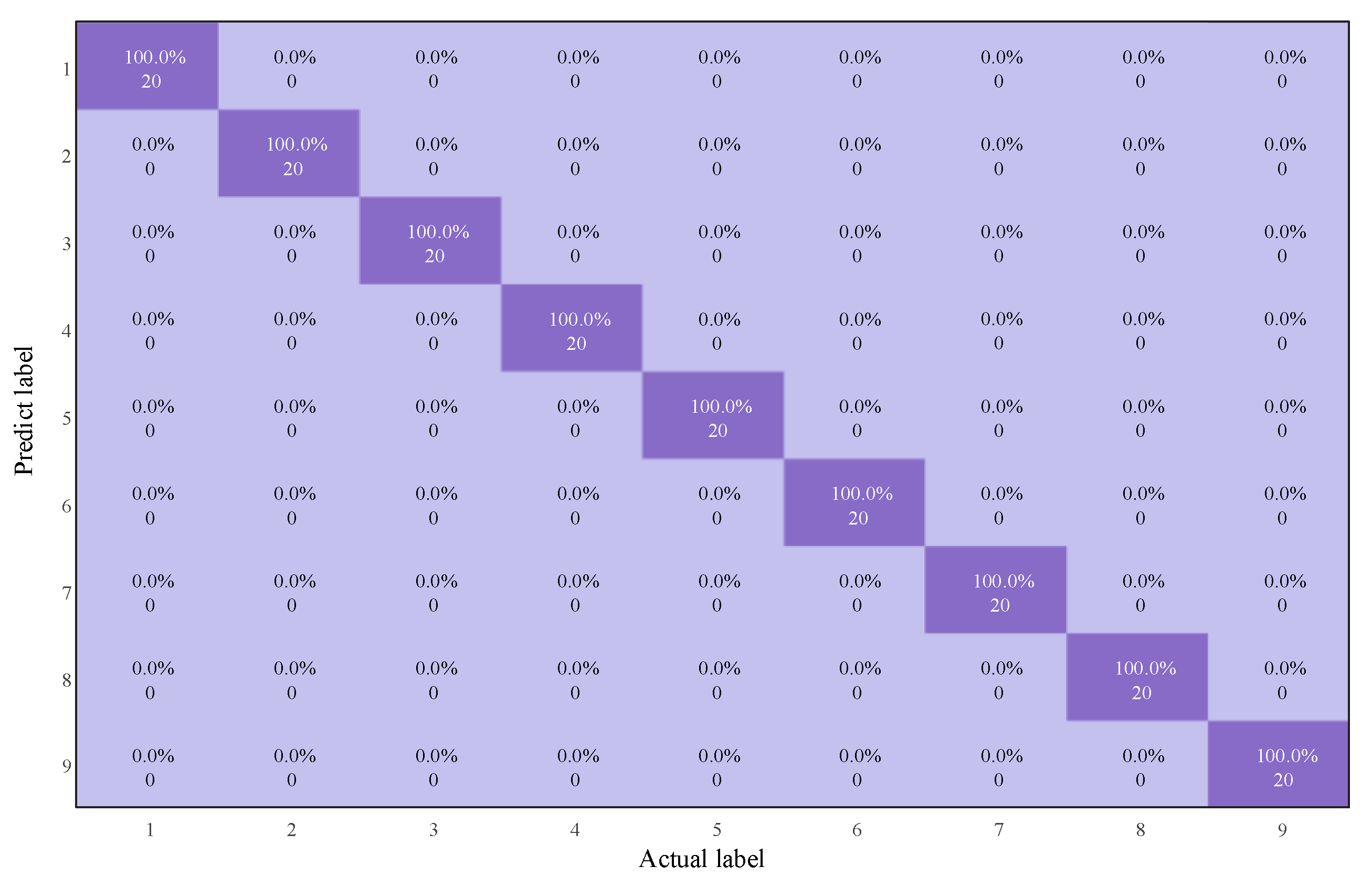
In 10 independent diagnostic experiments, the best diagnosis will identify 9 faults accurately without error, as shown in Figure 10. Comparative experiments will also be conducted with some of the commonly used methods of traditional circuit fault diagnosis. It has been found that due to the large scale of the dataset, there is a small difference within a short time interval, and the data contrast is not strong enough. Shallow neural networks often have certain limitations in feature extraction, especially when dealing with complex signals and high-dimensional data, where conventional feature extraction methods struggle to capture key information from the data. Therefore, it becomes particularly important to apply data preprocessing techniques. In this study, Wavelet Transform (WTF) and Principal Component Analysis (PCA) are chosen as the core steps for data preprocessing. WTF decomposes the signal into multiple frequency bands, effectively extracting both time-domain and frequency-domain features, especially suitable for noise and non-stationary signals. PCA, on the other hand, reduces dimensionality while retaining important features and removing redundant information, thus improving model efficiency and computational performance.
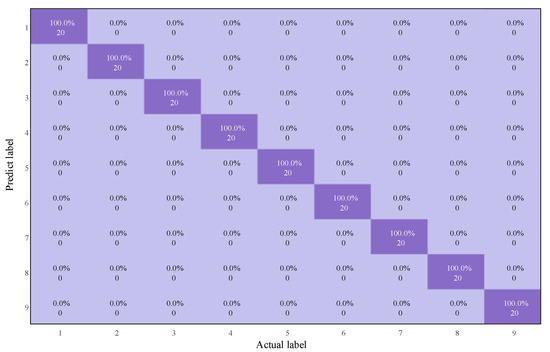
Figure 10.
The best result of diagnosis process of Butterworth low-pass filter based on ECA-MI-CNN.
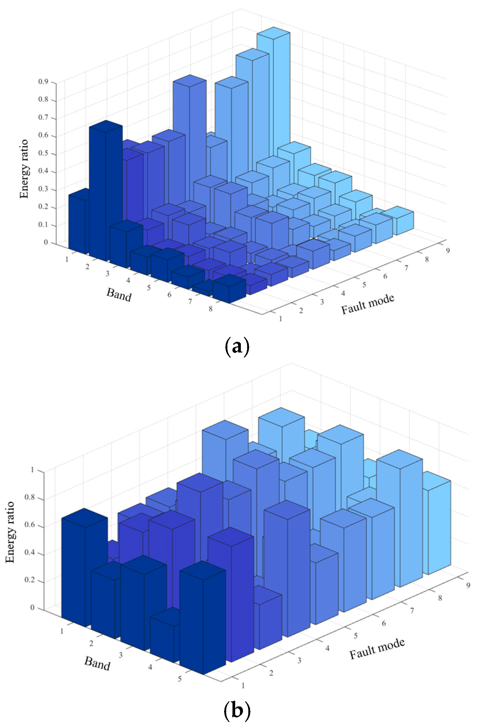
First, the original 9 types of fault signals are subjected to a three-level wavelet packet decomposition and extract the main features. As shown in Figure 11a, after the WTF decomposition of the nine types of faults, there is a clear difference in the energy share of each fault from band 1 to band 5, while there is no clear difference in the energy share of the nine types of faults from band 6 to band 8. PCA is then used to extract the most important features and reduce the dimensionality of the data, thereby reducing computational complexity, the energy share of the nine types of faults from band 1 to band 5 is shown in Figure 11b. Diagnostic experiments were conducted with shallow neural networks and compared with CNN and variants of CNN for diagnosis, and the model performance was judged by the average correct diagnosis rate and the average F1-Measure.

Figure 11.
Butterworth low-pass filter fault signal energy map. (a) Butterworth low-pass filter fault signal feature diagram, (b) Butterworth low-pass filter wavelet transform energy map and PCA characteristic energy map.
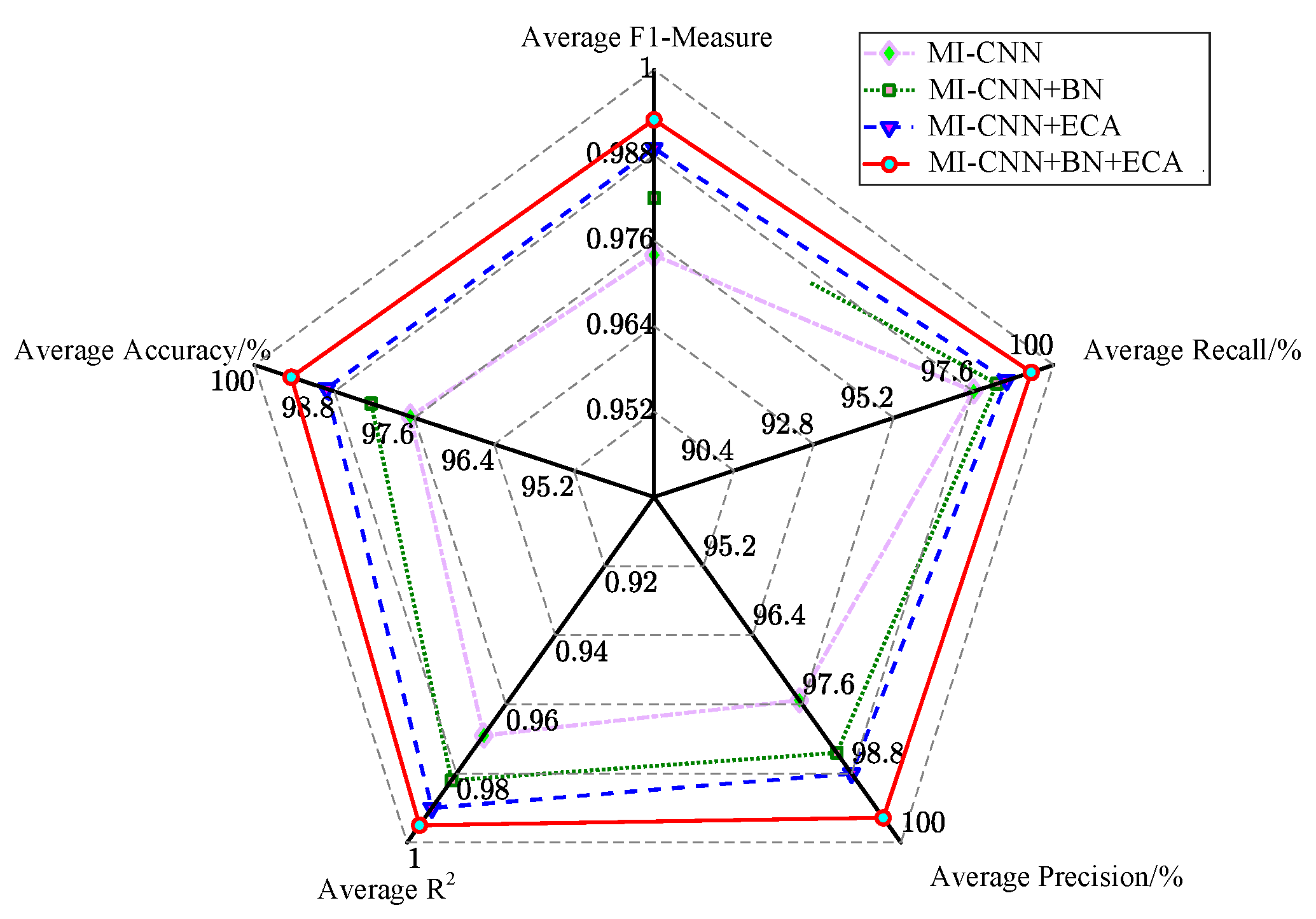
The results in Figure 12 and Table 2 show that in the 10 experimental tests with Butterworth low-pass filter, the fault diagnosis rate is above 92% for all methods except the one using ELM for classification, and the ECA-MI-CNN network works error-free four times, and its average correct rate is 99.37%. The MI-CNN network outperforms the CNN network, and by adding the squeeze and excitation network module and the convolutional block attention module, the fault diagnosis rates of both SENet-MI-CNN and CBAM-MI-CNN models were improved to different degrees (98.04%, 98.53%) compared to the MI-CNN model. The above experimental analysis indicates that the ECA added to the MI-CNN network can extract the main features more reasonably and improve the accuracy of fault diagnosis. However, due to the relatively simple structure of the Butterworth low-pass filter circuit, a high classification accuracy can also be achieved by using a shallow learning approach after the data have been processed. The simple circuit cannot highlight the advantages of the method proposed in this paper, so it is again validated with a composite circuit.
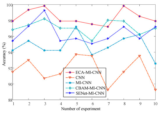
Figure 12.
Butterworth low-pass filter fault diagnosis accuracy curve.
Table 2.
Butterworth low-pass filter fault diagnosis comparison.
3.5. Diagnostic Results of Two-Stage Four Op-Amp Double-Order Low-Pass Filter
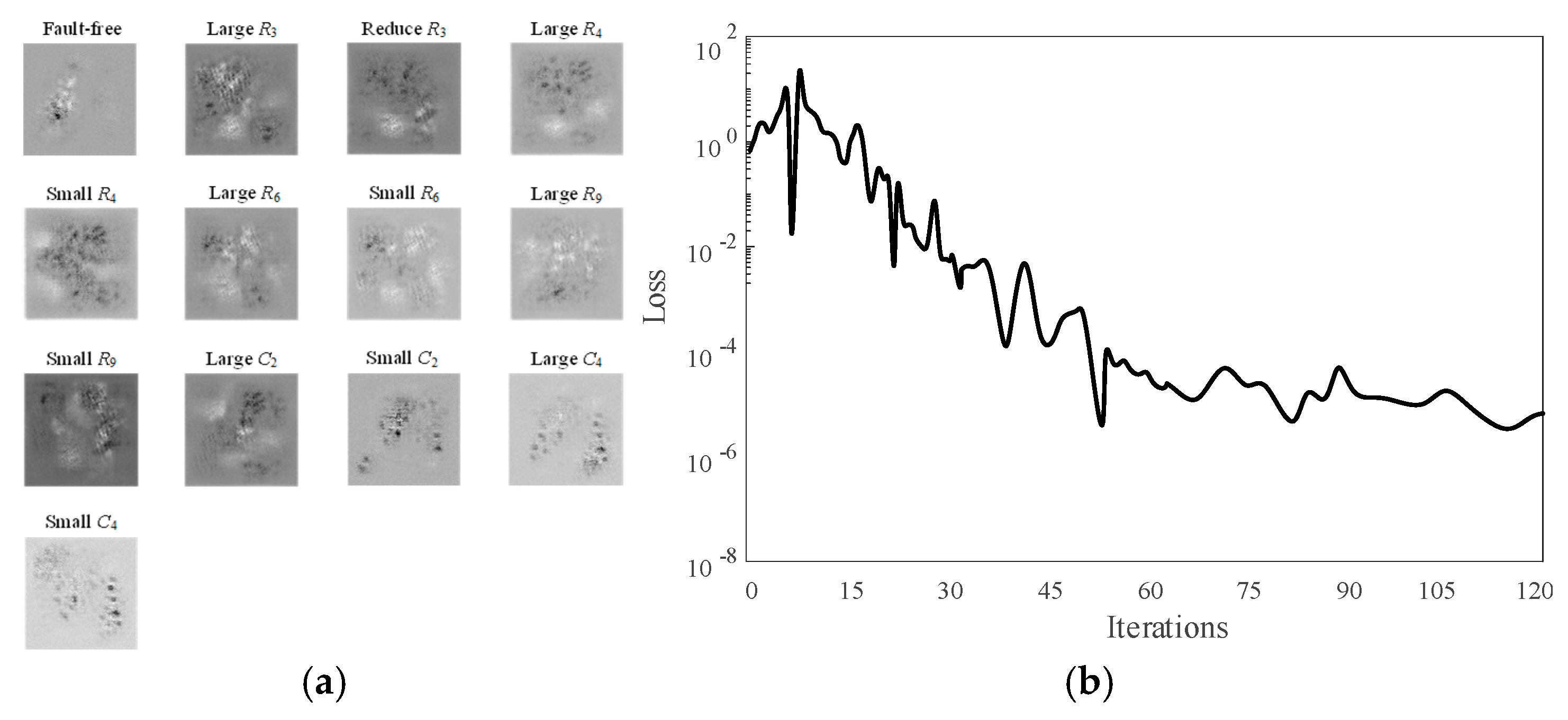
A more complex experimental circuit is used to further validate the effectiveness and superiority of the proposed network for fault diagnosis in complex circuits. The two-stage four op-amp double-order low-pass filter was used as the experimental circuit to verify the model performance. The same excitation signal as that of the Butterworth low-pass filter was applied to the circuit, and data were collected. Values of resistance and capacitance are considered normal if they vary within 5% above or below standard values, and are considered large or small if they are above or below 5%. Circuit fault diagnosis is carried out under the same experimental conditions. Based on the sensitivity tests, R3, R4, R6, and R9 in the resistors, and C2 and C4 in the capacitors, for a total of 13 categories of faults, were selected for model performance verification. A total of 13 categories of faults are shown in Table 3. Figure 13a shows a plot of the fault signal characteristics of a two-stage four op-amp double-order low-pass filter, from which it can be seen that the 13 classes of faults can be clearly identified. Figure 13b shows the relationship between the loss function and the number of iterations, with the final loss function stabilizing at approximately 10−6.
Table 3.
Fault modes of two-stage four op-amp double-order low-pass filter.
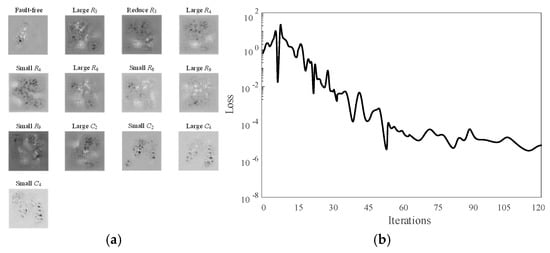
Figure 13.
Fault signal feature diagram and loss function diagram of two-stage four op-amp double-order low-pass filter: (a) two-stage four op-amp double-order low-pass filter fault signal feature diagram; (b) relationship diagram of iteration times and loss function.
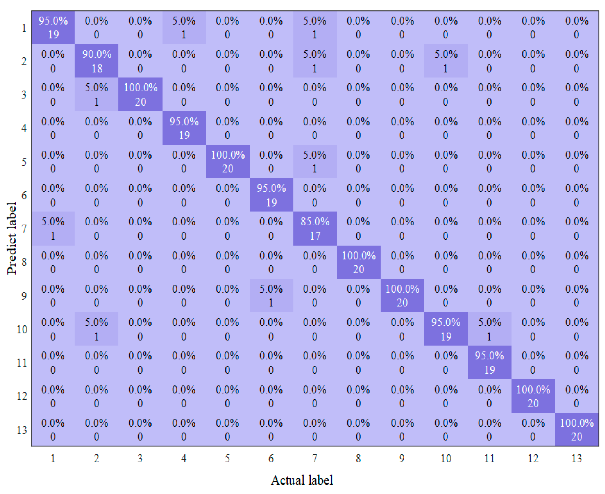
In the 10 diagnostic experiments of a two-stage four op-amp double-order low-pass filter, the highest diagnostic accuracy is shown in Figure 14:
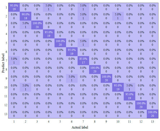
Figure 14.
The best result of diagnosis process of two-stage four op-amp double-order low-pass filter based on ECA-MI-CNN.
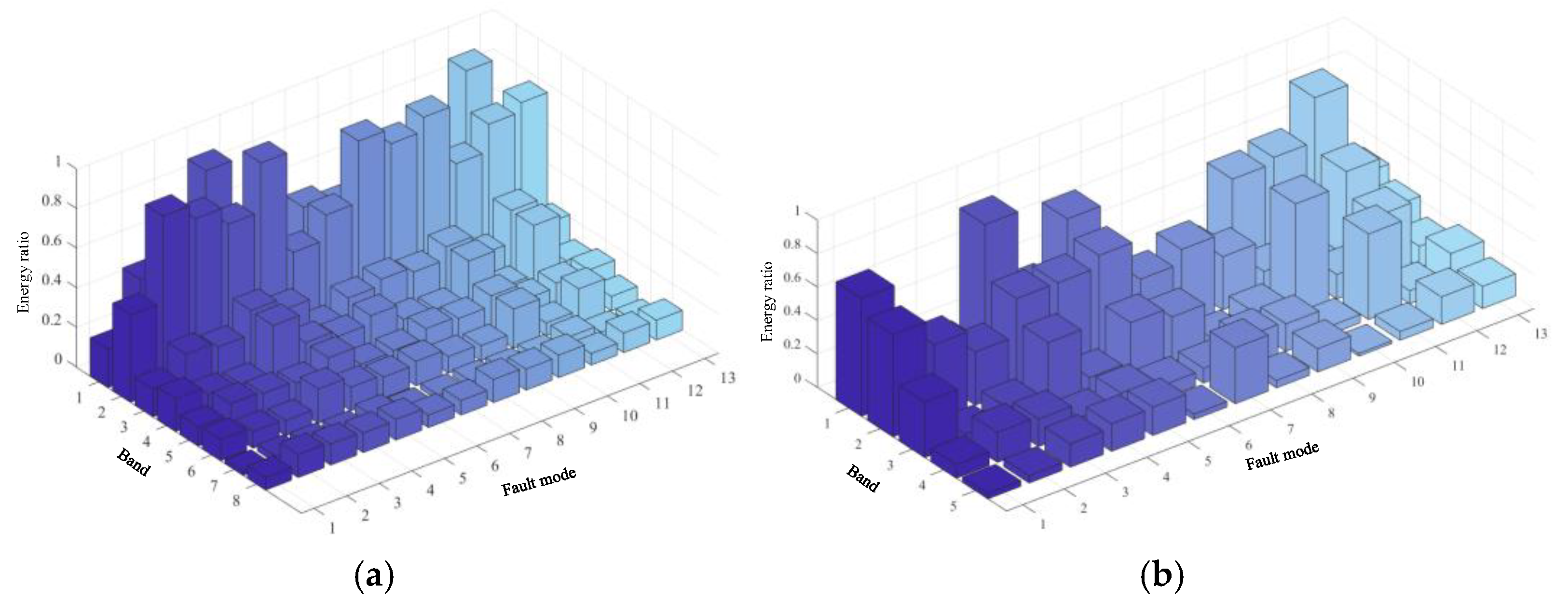
Similarly, to avoid the limitations in feature extraction of shallow machine learning methods, the data preprocessing method of WTF+PCA, as described in Section 3.2, was used in this experiment. Figure 15 represents the energy plots of different frequency bands after wavelet decomposition at different fault types and the energy plots of different frequency bands after PCA processing, respectively. From Figure 15, it can be seen that after three decompositions using WTF, the energy of 13 types of faults in different frequency bands from Band 1 to Band 4 are distinctly different, but from Band 5 to Band 8, the energy percentage of 13 types of faults is not much different, while using PCA processing not only reduces the dimensionality but also retains the original feature information, from the PCA energy percentage plot, it can be seen that the energy percentage of 13 types of faults from Band 1 to Band 5 The difference is relatively obvious, and the comparison results are shown in Table 4 and Figure 16.
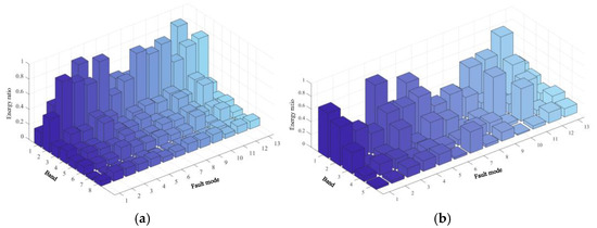
Figure 15.
The characteristic energy of the two-stage four op-amp double-order low-pass filter: (a) two-stage four op-amp double-order low-pass filter fault signal feature diagram; (b) two-stage four op-amp double-order low-pass filter PCA characteristic energy surface diagram.
Table 4.
Comparison of fault diagnosis of the two-stage four op-amp double-order low-pass filter.

Figure 16.
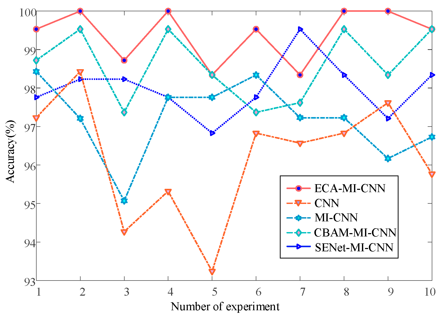
The fault diagnosis accuracy curve of the two-stage four op-amp double-order low-pass filter.
The average accuracy of the ECA-MI-CNN net-work model was 98.29% in 10 experimental tests of complex circuits, as can be obtained in Figure 16 and Table 4. The MI-CNN network optimized by SENet and CBAM outperformed the MI-CNN network, but was lower than the MI-CNN network with the ECA module. In contrast, only SVM was the best for shallow learning, with an average accuracy of 86.20%, but much lower than the ECA-MI-CNN proposed in this paper, and the other two methods were unable to achieve accurate classification of complex circuits.
Through the simulation experimental analysis of complex circuits, it can be seen that the ECA module reduces the complexity of the model while ensuring the model performance, while MI-CNN can effectively improve the defect of irreversible information loss caused by continuous convolution through the comprehensive capture of time domain feature information and frequency domain feature information. Through the combination of these two methods, it can not only avoid complicated data pre-processing, but also effectively extract and classify the features of complex circuits. Based on the results of comparison experiments, the method proposed in this paper has obvious advantages in complex circuits.
In addition, combined with Table 2 and Table 4, it can be seen that in the face of simple features in simple circuits, shallow learning can preprocess the data by WXT and PCA to select important features and reduce the dimensionality, thus satisfying the small data sample requirement of shallow learning and compensating for the lack of feature extraction capability to a certain extent. However, in the face of complex features in complex circuits, shallow learning can no longer apply data preprocessing operations to make up for its essential deficiencies, while deep learning has an absolute advantage in pinpointing fault features. Table 4 shows that the accuracy of MI-CNN is improved by 6.97% compared with CNN; this is because MI-CNN captures feature information from both time and frequency domains comprehensively. Meanwhile, the diagnostic accuracy of the three models, SENet-MI-CNN, CBAM-MI-CNN, and ECA-MI-CNN, is improved by 0.27%, 2.52%, and 3.63%, respectively, compared with the MI-CNN model. The performance of the CBAM-MI-CNN model is better than SENet-MI-CNN, which is because CBAM fuses both channel and spatial features with SENet for more reasonable feature extraction, and ECA module can achieve information interaction by not reducing the dimensionality compared with CBAM module to ensure the reasonableness and accuracy of feature extraction.
4. Comparative Experiments of Model Performance
4.1. ECA Parameter Selection Experiments
To evaluate the impact of the interaction range parameter k on the performance of the ECA module, we conducted a series of experiments with varying values of k. The objective of these experiments was to analyze how the choice of k influences the model’s ability to capture the dependencies and correlations between input features. According to the relationship between the value of k and the number of channels described in Section 2.3, the theoretical calculation gives k when the number of channels is 128. However, since k needs to be the nearest odd number, we selected k and k for the experiments. Additionally, to further analyze the impact of k on model performance, we included k = 1 and k = 7 as comparison groups to observe how different interaction ranges affect the model’s feature extraction capability.
We conducted an experimental analysis on the impact of different k values in the ECA module on model performance, and the results are shown in Table 5. From the experimental results, it can be observed that as k increases, the model’s diagnostic accuracy and F1-Measure initially improve and then decline. When k = 1, the model achieves an accuracy of 98.24% and an F1-Measure of 0.979, indicating that a small k value has limitations in capturing feature interactions, making it insufficient to fully extract dependencies between features.
Table 5.
The impact of different k values on model performance.
When k increases to 3, the model performance reaches its peak, with accuracy improving to 99.21% and the F1-Measure reaching 0.990. This suggests that an appropriate increase in k helps the model capture broader feature relationships and enhances classification performance. However, when k is further increased to 5, the accuracy (99.02%) and F1-Measure (0.987) show a slight decline, and when k is increased to 7, the model performance further decreases (Accuracy = 98.42%, F1-Measure = 0.982).
These results indicate that an excessively large k value may introduce too much irrelevant or redundant information, reducing the effectiveness of feature interactions and ultimately impacting classification performance. Therefore, in this experiment, k = 3 is the optimal choice, achieving a good balance between capturing feature dependencies and avoiding information redundancy.
4.2. Feature Distribution Experiment
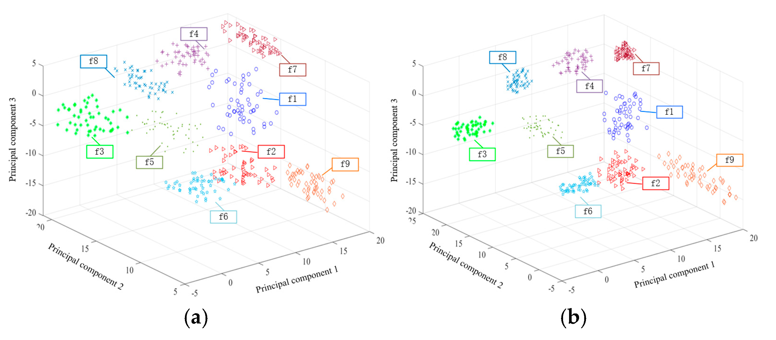
In order to prove that the MI-CNN model is superior to CNN in learning different types of features, Butterworth low-pass filter is used to for experimental verification, and kernel principal component analysis (KPCA) dimension-reduction algorithm is adopted for feature visualization. Figure 17 is the comparison diagram of feature classification, in which Figure 17a is the classification result of the CNN model, from which it can be seen that f1 and F2 overlap and the distribution of the same type of faults are scattered. After using the MI-CNN model to fuse time domain information and frequency domain information, the classification result is shown in Figure 17b, from which it can be seen that F2 data are close to F1 and F6, but there is no overlap phenomenon, and other fault types can be accurately distinguished. Moreover, the distribution of the same type of faults is more compact than that in Figure 17a, which is consistent with the classification results of the model.
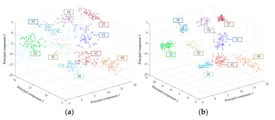
Figure 17.
Visual distribution of features: (a) feature distribution diagram based on CNN; (b) feature distribution diagram based on MI-CNN.
4.3. Experimental Verification of Learning Rate
As a hyperparameter, the learning rate is used to update the weight in the process of gradient descent. A low learning rate can ensure the retention of local minimum, but the longer training process is easy to cause over-fitting. High learning rates can cause the same problems.
To solve the above problem, we set the decay factor , the period to t, and the learning rate was multiplied by one every other cycle. The expression is:
where , and t = 2.
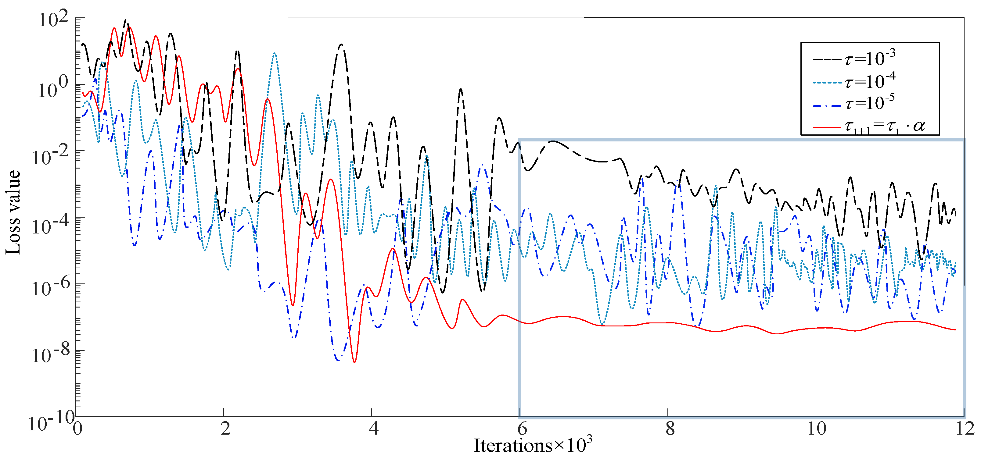
However, in actual training, most learning rates are empirical values. To verify the excellence of the learning rate decay, the commonly used empirical values of ,, and are compared with the decaying learning rate. Figure 18 is the training error curve diagram.
Figure 18.
Comparison results of ablation performance.
It can be seen from Figure 19 that the loss value using the decay learning rate is not the lowest when the ECA-MI-CNN model is initially trained, and the training error is the lowest and stabilizes (Loss = 10−8) after about 6000 steps of training. However, when the model is trained with other fixed learning rates, the training error is still fluctuating after 6000 steps of training, where the largest loss is (Loss = 10−3), when and both have almost equal (Loss = 10−5) loss.
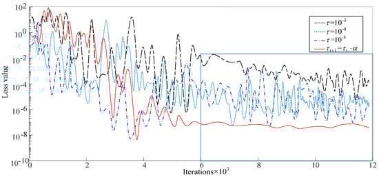
Figure 19.
Relationship between learning rate and loss function.
The reason for this is because the decay learning rate is fast in the initial stage, which can accelerate the convergence of the network. However, as the number of training cycles increases, the learning rate slows down, and after fine-tuning the weights, a more reasonable feature distribution is obtained, while a fixed value of the learning rate does not slow down with the increase in the number of iterations, and the comparative analysis in Figure 19 demonstrates the importance of a reasonable learning rate for the model.
4.4. Model Robustness Verification
- (1)
- Noise experiments on the Butterworth low-pass filter
To verify the robustness of the ECA-MI-CNN model, white noise at 5 dB, 15 dB, and 20 dB was added to the Butterworth low-pass filter test set, and the final classification results of the model are shown in Table 6. As seen in Table 6, the ECA-MI-CNN model can still achieve accurate classification under the influence of high-intensity noise. The multi-channel classification of MI-CNN extracts time-domain features and uses the ECA module to fully extract feature information from the original signal. Additionally, the spectral data exhibits better clustering performance and stronger anti-interference capabilities. Therefore, the ECA-MI-CNN model shows clear advantages and good robustness in noise testing, as shown in Figure 20.
Table 6.
Experimental results of Butterworth low-pass filter with noise.
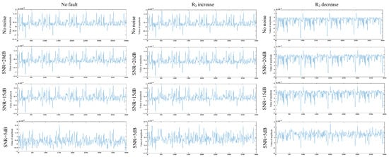
Figure 20.
Time domain and frequency domain diagrams under different noises.
- (2)
- Noise experiments on two-stage four op-amp double-order low-pass filter
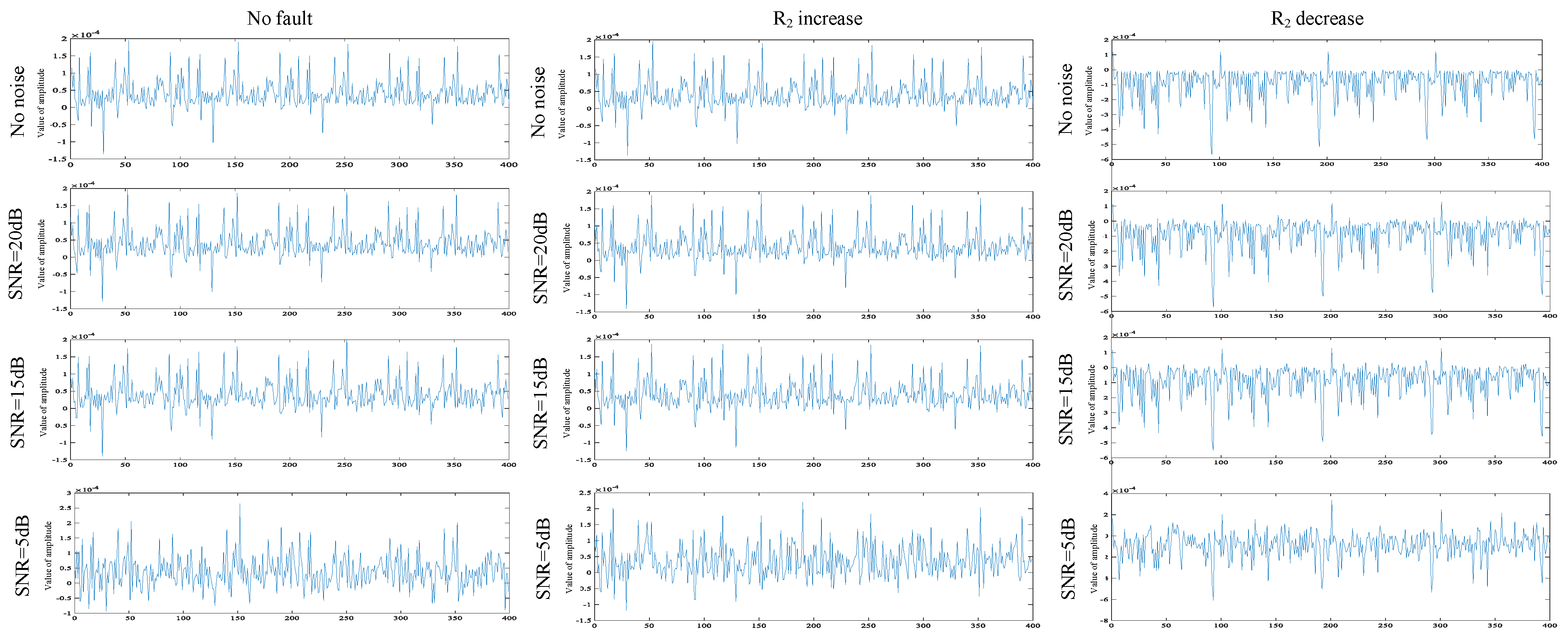
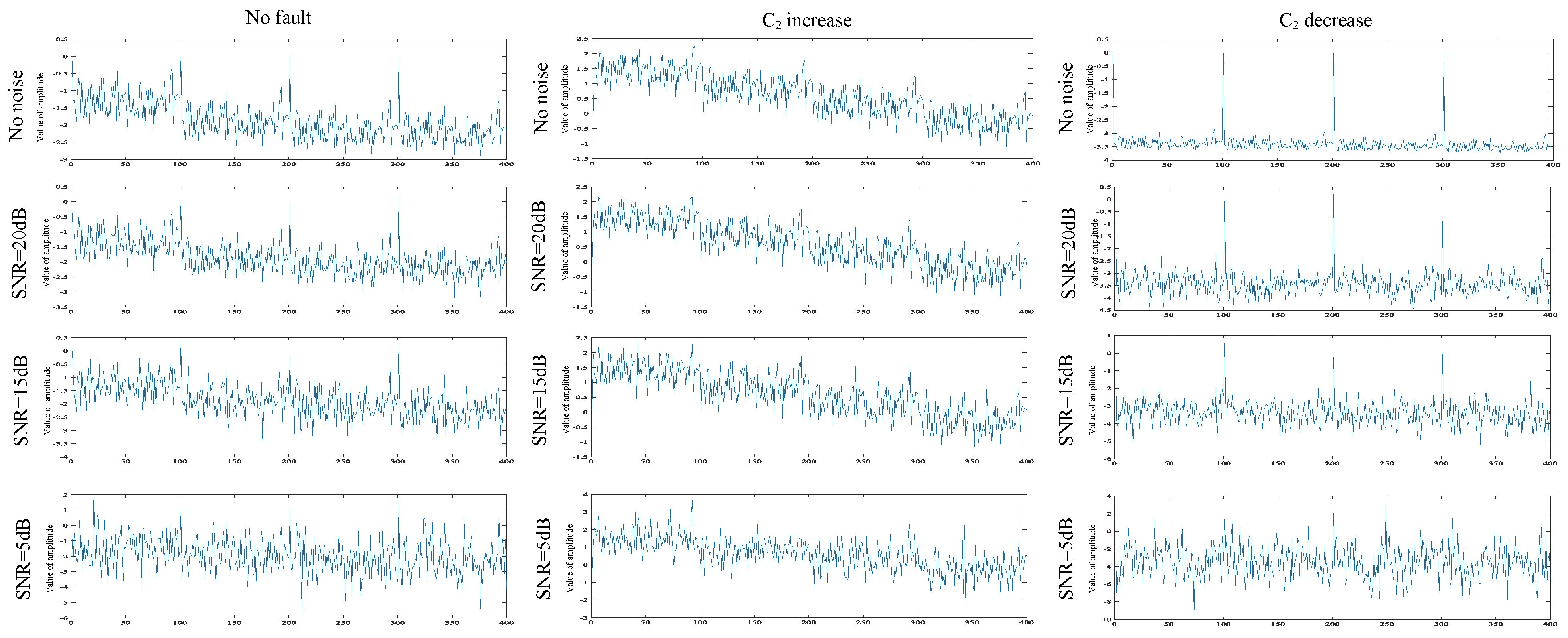
To further evaluate the robustness of the ECA-MI-CNN model, additional noise experiments were conducted using a second-order low-pass filter with two-stage four op-amp double-order low-pass filter. Similar to the Butterworth low-pass filter test, white noise at 5 dB, 15 dB, and 20 dB was added to the signal, and signal plots under different noise levels and fault conditions were analyzed, as shown in Figure 21.
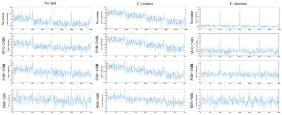
Figure 21.
Time domain and frequency domain diagrams under different noises.
The experimental results presented in Table 7 demonstrate that the ECA-MI-CNN model exhibits good robustness and effectiveness under varying noise levels. In the noiseless scenario, the model achieved an impressive accuracy of 98.24%, indicating its excellent performance in ideal conditions. Although the diagnostic accuracy is slightly lower than that of the Butterworth low-pass filter after the introduction of noise, the ECA-MI-CNN model still maintains strong classification ability. When 20 dB white noise was introduced, the accuracy decreased to 91.57%; with 15 dB and 5 dB noise, the accuracy was 83.22% and 69.66%, respectively. These results show that, despite the decrease in accuracy due to noise, the ECA-MI-CNN model still demonstrates remarkable robustness and can accurately classify signals in challenging noisy environments. Therefore, although the diagnostic accuracy of the model is slightly lower than that of the Butterworth low-pass filter, it still performs well under noise and environmental interference, proving its effectiveness in real-world applications.
Table 7.
Experimental results of two-stage four op-amp double-order low-pass filter with noise.
5. Overview of the Study
In this paper, the effectiveness of the proposed method is verified through diagnostic experiments on a real analog circuit, specifically the Butterworth low-pass filter shown in Figure 22. The component parameters used in the physical circuit are detailed in Figure 5, and the fault modes are set as shown in Table 1. This allows for testing the performance of the ECA-MI-CNN diagnostic model under different conditions.
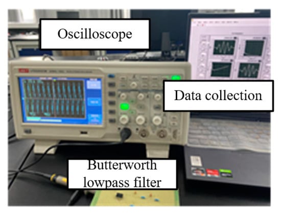
Figure 22.
Experimental facilities.
The specific steps are as follows:
- (1)
- Detect the output voltage and transmit it to LabView with NI acquisition card.
- (2)
- Collect 60,000 data points for each fault, resulting in 51,529 sample data points, set the offset to 100, and 80 fault samples can be made, thus totaling 720 samples.
- (3)
- Partition training samples and test samples according to the ratio of 7:3.
- (4)
- Train and evaluate the model performance.
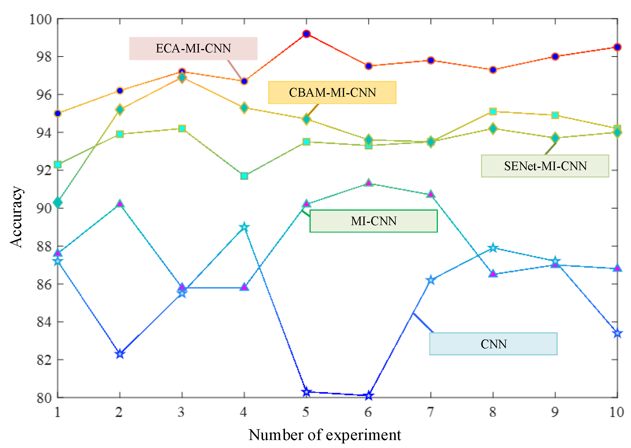
In the actual experimental verification, 10 independent diagnostic experiments were conducted to reduce the impact of randomness on the results, as shown in Figure 23. It was found that, under the action of the excitation signal, the original signal in the real environment is inevitably affected by noise, environmental factors, and other influences, which results in a slightly longer operating time compared to the simulation experiments and slightly affects the classification results. Therefore, the performance of the proposed model in practical applications is slightly lower than that of the simulation experiments. As shown in Table 8, the average diagnostic accuracy of the proposed method is 97.32%, significantly higher than CBAM-MI-CNN (94.86%), Squeeze-and-Excitation Network-MI-CNN (94.27%), MI-CNN (88.31%), and traditional CNN (84.29%).
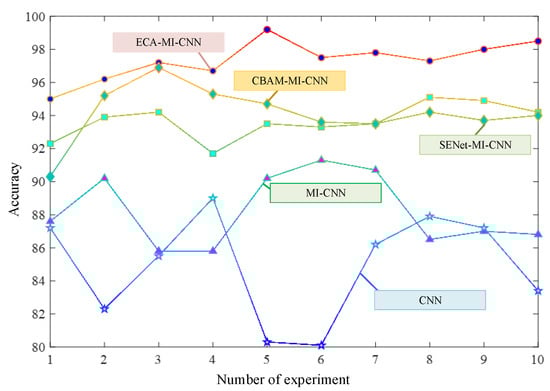
Figure 23.
Butterworth low-pass filter fault diagnosis accuracy curve.
Table 8.
Butterworth low-pass filter actual fault diagnosis mean comparison.
In addition, Table 8 shows that the ECA-MI-CNN diagnostic model takes the least time (4.93 s), followed by CBAM-MI-CNN and SENet-MI-CNN (5.72 s and 6.27 s), with MI-CNN and CNN taking the longest time (10.06 s and 12.87 s). The experiments demonstrate that the diagnostic performance of the model can be improved by adding the attention mechanism. However, the fully connected layers inside the SENet and CBAM modules result in a higher number of parameters compared to ECA, which explains why CBAM-MI-CNN and SENet-MI-CNN models perform worse than the proposed model in diagnostic performance.
Further analysis reveals that while the CBAM model outperforms SENet in some tasks, it still falls short compared to the ECA model. In CBAM, both spatial and channel attention mechanisms are introduced simultaneously, which helps enhance the feature representation ability. However, due to the complex structure, the computational cost is higher, resulting in greater computational overhead in practical applications. In contrast, ECA simplifies the attention calculation across channels, maintaining strong classification performance while ensuring efficiency. Therefore, the ECA model not only has advantages in diagnostic accuracy but also offers higher computational efficiency, making it a more ideal choice.
When a circuit is operated for a long time, the circuit parameters are shifted, making the data contain cumulative noise that may affect the diagnostic performance of the network. To verify the robustness of the model, a Butterworth low-pass filter is continuously energized for three days, and then 16,000 sets of circuit fault data are randomly collected, and the ECA-MI-CNN model is enhanced by overlapping sampling to perform signal feature extraction and diagnosis in a noisy background. As can be seen from Table 9, the average diagnostic accuracy of the ECA-MI-CNN model is 96.83%, which is still better than CBAM-MI-CNN (94.82%), SENet-MI-CNN (93.85%), MI-CNN (85.94%), and conventional CNN (83.81%). The performance of ECA-MI-CNN did not degrade significantly due to the accumulated noise of Butterworth low-pass filter after long time operation. It indicates that ECA has good noise immunity with obvious advantages over CBAM and SENet.
Table 9.
Comparison of actual fault diagnosis of Butterworth low-pass filter for long time operation.
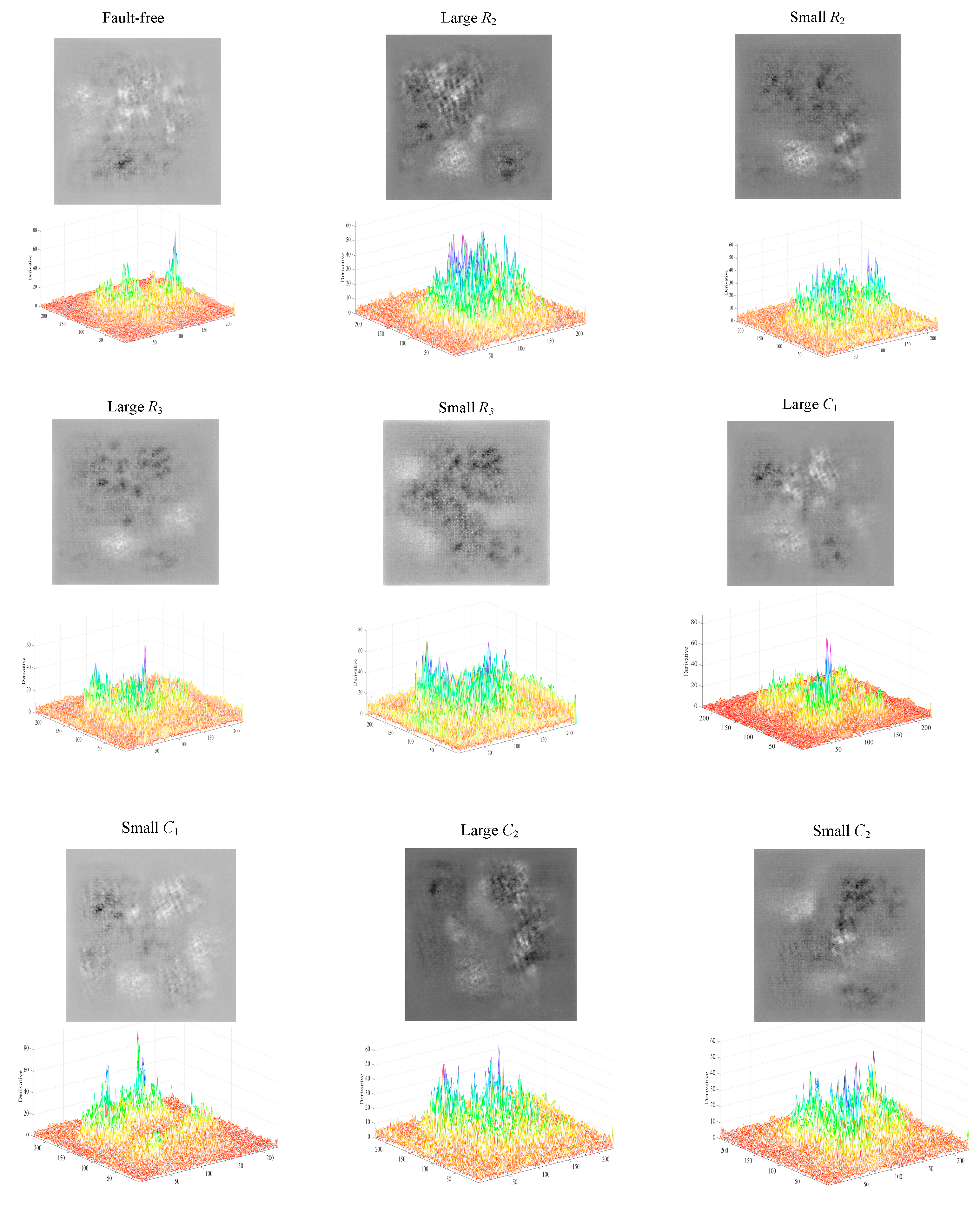
Figure 24 shows a plot of the fault features and feature edge intensities diagnosed by the ECA-MI-CNN model under the condition of long-time operation of the Butterworth low-pass filter, and the edge intensities of the nine features are calculated by the Canny operator. The edge intensity is expressed as the squared error of the partial derivatives, and the higher the peak of the edge intensity, the more distinct the fault feature is. From Figure 24, it can be seen that the nine fault features of Butterworth low-pass filter have a large degree of difference from each other.

Figure 24.
Butterworth low-pass filter feature and edge strength diagram.
Therefore, it can be proved that the method proposed in this paper can effectively diagnose circuit faults, and can still tap the deep essential features without considering the influence of the environment on the actual circuit signal and the interference of the accumulated noise brought by the long-term operation of the circuit, which has good anti-interference ability and high practical application value, proving the robustness of the model.
6. Conclusions
In this paper, an ECA-MI-CNN analog circuit fault diagnosis model is proposed by combining the attention mechanism with a neural network. The main conclusions are as follows:
- (1)
- Overlap sampling of enhanced sample data for enhanced generalization performance of deep neural nets;
- (2)
- Unlike traditional CNN networks, the MI-CNN model can combine time domain information and frequency domain information, which can improve the shortcoming of mining essential features due to the loss of detailed information caused by continuous CNN. It is more suitable for deep feature extraction in complex circuits.
- (3)
- The MI-CNN model is optimized with the ECA module and BN layer to simplify the model while accelerating the convergence of the network. A comparison of the optimized network model with squeeze-and-excitation networks and the CBAM module demonstrates that ECA has a significant advantage in terms of fault feature information and is able to perform fault diagnosis quickly and accurately.
Deep learning-based fault diagnosis methods, with their unique advantages, will undoubtedly become an indispensable key technology in future intelligent diagnostic technologies. Future research on such methods should primarily focus on the following aspects:
- (1)
- From the perspective of complementary advantages, it is highly meaningful to construct a new hybrid intelligent diagnostic method for in-depth research, and thus worthwhile exploring. The following aspects should be considered: the combination of deep learning and shallow networks, and the combination of model-based approaches and data-driven approaches.
- (2)
- Fault diagnosis technology for analog circuits cannot remain at the experimental research stage; it must become a practical tool that can be applied in real-world scenarios. Therefore, future research should consider both industrial practice and academic perspectives, taking into account environmental, cost, and practicality factors.
- (3)
- The application of time-frequency fusion in chaotic systems holds significant potential, as it can provide more precise analysis tools for the dynamic behavior and nonlinear characteristics of chaotic systems. Future research should explore the integration of time-frequency analysis techniques with deep learning methods to enhance their application in fault diagnosis of chaotic systems.
Author Contributions
Investigation and Methodology, H.Y.; Writing—review and editing, L.L., G.L. and Y.S.; Investigation and editing, J.Z. and Z.W. All authors have read and agreed to the published version of the manuscript.
Funding
This research was funded by the Scientific and Technological Project of Gansu Province (24CXGA042); the National Science Foundation of China (62263019); the Gansu Provincial Science and Technology Program (22YF7FA166, 22YF7GA164).
Data Availability Statement
All data are included in this paper.
Conflicts of Interest
The authors declare no conflicts of interest.
References
- Vasan, A.S.S.; Long, B.; Pecht, M. Diagnostics and prognostics method for analog electronic circuits. IEEE Trans. Ind. Electron. 2012, 60, 5277–5291. [Google Scholar] [CrossRef]
- Khemani, V.; Azarian, M.H.; Pecht, M. WavePHMNet: A comprehensive diagnosis and prognosis approach for analog circuits. Adv. Eng. Informatics 2024, 59, 102323. [Google Scholar] [CrossRef]
- Wang, L.; Liu, Z.Q. Fault diagnosis of analog circuit for WPA-IGA-BP neural network. Syst. Eng. Electron. 2021, 43, 1133–1143. [Google Scholar]
- Jia, R.; Wang, J.; Zhou, J. Fault diagnosis of industrial process based on the optimal parametric t-distributed stochastic neighbor embedding. Sci. China Inf. Sci. 2020, 64, 159204. [Google Scholar] [CrossRef]
- Gao, M.Z.; Xu, A.Q.; Tang, X.F.; Zhang, W. Analog circuit diagnostic method based on multi-kernel learning multiclass rele-vance vector machine. Acta Autom. Sin. 2019, 45, 434–444. [Google Scholar]
- Zhang, S.; Chang, Y.; Li, H.; You, G. Research on Building Energy Consumption Prediction Based on Improved PSO Fusion LSSVM Model. Energies 2024, 17, 4329. [Google Scholar] [CrossRef]
- Yang, C. Parallel–series multiobjective genetic algorithm for optimal tests selection with multiple constraints. IEEE Trans. Instrum. Meas. 2018, 67, 1859–1876. [Google Scholar] [CrossRef]
- Li, Y.; Dong, J. Fault Detection Unknown Input Observer for Local Nonlinear Fuzzy Autonomous Ground Vehicles System Based on a Joint Peak-to-Peak Analysis and Zonotopic Analysis Threshold. IEEE Trans. Veh. Technol. 2025, 7, 1–11. [Google Scholar] [CrossRef]
- Ding, J.; Zhang, H.; Tong, Q.Y.; Chen, Z. Studies of phase return map and symbolic dynamics in a periodically driven Hodgkin–Huxley neuron. Chin. Phys. B 2014, 23, 020501. [Google Scholar] [CrossRef]
- Wang, J.; Li, T.; Sun, C.; Yan, R.; Chen, X. Improved spiking neural network for intershaft bearing fault diagnosis. J. Manuf. Syst. 2022, 65, 208–219. [Google Scholar] [CrossRef]
- Wang, G.; Xue, L.; Zhu, Y.; Zhao, Y.; Jiang, H.; Wang, J. Fault diagnosis of power-shift system in continuously variable transmission tractors based on improved echo state network. Eng. Appl. Artif. Intell. 2023, 126, 106852. [Google Scholar] [CrossRef]
- Aminian, M.; Aminian, F. Neural-network based analog-circuit fault diagnosis using wavelet transform as preprocessor. IEEE Trans. Circuits Syst. II-Analog. Digit. Signal Process. 2000, 47, 151–156. [Google Scholar] [CrossRef]
- Binu, D.; Kariyappa, B.S. RideNN: A New Rider Optimization Algorithm-Based Neural Network for Fault Diagnosis in Analog Circuits. IEEE Trans. Instrum. Meas. 2018, 68, 2–26. [Google Scholar] [CrossRef]
- Zhang, A.; Chen, C.; Jiang, B. Analog circuit fault diagnosis based UCISVM. Neurocomputing 2016, 173, 1752–1760. [Google Scholar] [CrossRef]
- Lu, Z.; Chu, Z.; Zhu, M.; Dong, X. Unsupervised feature learning using locality-preserved auto-encoder with complexity-invariant distance for intelligent fault diagnosis of machinery. Appl. Intell. 2025, 55, 379. [Google Scholar] [CrossRef]
- Wang, B.; Lei, Y.; Li, N.; Wang, W. Multiscale Convolutional Attention Network for Predicting Remaining Useful Life of Machinery. IEEE Trans. Ind. Electron. 2020, 68, 7496–7504. [Google Scholar] [CrossRef]
- Otele, C.G.A.; Onabid, M.A.; Assembe, P.S. Design and implementation of an Automatic Deep Stacked Sparsely Connected Convolutional Autoencoder (ADSSCCA) neural network for remote sensing lithological mapping using calculated dropout. Earth Sci. Informatics 2024, 17, 1993–2010. [Google Scholar] [CrossRef]
- Fang, F.; Li, L.; Gu, Y.; Zhu, H.; Lim, J.-H. A novel hybrid approach for crack detection. Pattern Recognit. 2020, 107, 107474. [Google Scholar] [CrossRef]
- Shelhamer, E.; Long, J.; Darrell, T. Fully convolutional networks for semantic segmentation. IEEE Trans. Pattern Anal. Mach. Intell. 2016, 39, 640–651. [Google Scholar] [CrossRef]
- Cui, J.; Wang, Y. A novel approach of analog circuit fault diagnosis using support vector machines classifier. Measurement 2011, 44, 281–289. [Google Scholar] [CrossRef]
- Mohamed, A.E.; Dahl, G.E.; Hinton, G. Acoustic modeling using deep belief networks. IEEE Trans. Audio Speech Lang. Process. 2011, 20, 14–22. [Google Scholar] [CrossRef]
- Wang, Z.; Wang, J.; Wang, Y. An intelligent diagnosis scheme based on generative adversarial learning deep neural networks and its application to planetary gearbox fault pattern recognition. Neurocomputing 2018, 310, 213–222. [Google Scholar] [CrossRef]
- Chen, Y.; Zhao, X.; Jia, X. Spectral-spatial classification of hyperspectral data based on deep belief network. IEEE J. Sel. Top. Appl. Earth Obs. Remote Sens. 2015, 8, 2381–2392. [Google Scholar]
- Su, X.; Cao, C.; Zeng, X.; Feng, Z.; Shen, J.; Yan, X.; Wu, Z. Application of DBN and GWO-SVM in analog circuit fault diagnosis. Sci. Rep. 2021, 11, 7969. [Google Scholar] [CrossRef]
- Lee, H.; Grosse, R.; Ranganath, R.; Ng, A.Y. Unsupervised learning of hierarchical representations with convolutional deep belief networks. Commun. ACM 2011, 54, 95–103. [Google Scholar] [CrossRef]
- Goodfellow, I.; Pouget-Abadie, J.; Mirza, M.; Xu, B.; Warde-Farley, D.; Ozair, S.; Courville, A.; Bengio, Y. Generative adversarial networks. Commun. ACM 2020, 63, 139–144. [Google Scholar] [CrossRef]
- Zhang, Y.; Li, W.; Sun, W.; Tao, R.; Du, Q. Single-source domain expansion network for cross-scene hyperspectral image classification. IEEE Trans. Image Process. 2023, 32, 1498–1512. [Google Scholar] [CrossRef]
- He, W.; He, Y.; Li, B. Generative adversarial networks with comprehensive wavelet feature for fault diagnosis of analog circuits. IEEE Trans. Instrum. Meas. 2020, 69, 6640–6650. [Google Scholar] [CrossRef]
- Kim, H.; Shin, J.W. Target exaggeration for deep learning-based speech enhancement. Digit. Signal Process. 2021, 116, 103109. [Google Scholar] [CrossRef]
- Du, T.; Zhang, H.; Wang, L. Analogue circuit fault diagnosis based on convolution neural network. Electron. Lett. 2019, 55, 1277–1279. [Google Scholar] [CrossRef]
- Zhang, C.; Zha, D.; Wang, L.; Mu, N. A novel analog circuit soft fault diagnosis method based on convolutional neural network and backward difference. Symmetry 2021, 13, 1096. [Google Scholar] [CrossRef]
- Wei, S.; Qu, Q.; Wu, Y.; Wang, M.; Shi, J. PRI modulation recognition based on squeeze-and-excitation networks. IEEE Commun. Lett. 2020, 24, 1047–1051. [Google Scholar] [CrossRef]
- Bi, X.; Xing, J. Multi-scale weighted fusion attentive generative adversarial network for single image de-raining. IEEE Access 2020, 8, 69838–69848. [Google Scholar] [CrossRef]
- Rawat, W.; Wang, Z. Deep Convolutional Neural Networks for Image Classification: A Comprehensive Review. Neural Com-Putation 2017, 29, 2352–2449. [Google Scholar] [CrossRef]
- He, K.; Zhang, X.; Ren, S.Q.; Sun, J. Deep Residual Learning for Image Recognition. In Proceedings of the IEEE Conference on Computer Vision and Pattern Recognition, Las Vegas, NV, USA, 27 June 2016; pp. 770–778. [Google Scholar]
- Zhou, R.; Chang, X.; Shi, L.; Shen, Y.-D.; Yang, Y.; Nie, F. Person reidentification via multi-feature fusion with adaptive graph learning. IEEE Trans. Neural Networks Learn. Syst. 2019, 31, 1592–1601. [Google Scholar] [CrossRef]
- Tong, G.; Li, Y.; Gao, H.; Chen, H.; Wang, H.; Yang, X. MA-CRNN: A multi-scale attention CRNN for Chinese text line recognition in natural scenes. Int. J. Doc. Anal. Recognit. (IJDAR) 2019, 23, 103–114. [Google Scholar] [CrossRef]
- Tang, H.; Gao, S.; Wang, L.; Li, X.; Li, B.; Pang, S. A novel intelligent fault diagnosis method for rolling bearings based on wasserstein generative adversarial network and convolutional neural network under unbalanced dataset. Sensors 2021, 21, 6754. [Google Scholar] [CrossRef]


Disclaimer/Publisher’s Note: The statements, opinions and data contained in all publications are solely those of the individual author(s) and contributor(s) and not of MDPI and/or the editor(s). MDPI and/or the editor(s) disclaim responsibility for any injury to people or property resulting from any ideas, methods, instructions or products referred to in the content. |
© 2025 by the authors. Licensee MDPI, Basel, Switzerland. This article is an open access article distributed under the terms and conditions of the Creative Commons Attribution (CC BY) license (https://creativecommons.org/licenses/by/4.0/).