Abstract
Structural Topology Optimisation (STO) plays a critical role in computational engineering, enabling the creation of material-efficient, performance-driven structures. However, dynamic STO workflows, particularly those involving time-varying or seismic excitations, are often inaccessible to architects and engineers due to their reliance on standalone solvers, large-scale data handling, and advanced programming skills. This paper introduces a Computer-Aided Design (CAD)-embedded, time-dependent STO framework built upon a modular, adjoint-based optimisation core integrated into a Visual Programming Language (VPL) interface. Implemented within a parametric CAD environment through a custom C# component, the framework embeds a MATLAB-based solver to support geometry definition, boundary condition control, and dynamic finite element analysis under harmonic and seismic loading. The resulting Graphical User Interface (GUI) lowers technical barriers by enabling users to iteratively configure STO parameters, manage meshing, and visualise real-time results. Case studies on tall building façades under earthquake excitation validate the framework’s ability to minimise displacement at targeted Degrees of Freedom (DOFs), dynamically adapt material distributions, and enhance structural resilience. By bridging high-fidelity computational methods with accessible visual workflows, the proposed system advances the integration of dynamic STO into both architectural and engineering practice.
1. Introduction
Designers and engineers increasingly rely on CAD environments to develop, analyse, and refine complex geometries. Tools such as Rhinoceros3D and its Grasshopper (GH) add-on facilitate a VPL approach, wherein users can expeditiously explore parametric forms without extensive or complex scripting. Notwithstanding these advancements, the integration of high-level Structural Optimisation (SO), particularly under dynamic loading conditions, remains an unresolved challenge. The majority of Topology Optimisation (TO) methods operate in stand-alone solvers, necessitating advanced coding skills and intricate data exchanges that impede iterative design processes [1,2,3]. Recent studies underscore the value of TO for material efficiency, lightweight structures, and performance-driven design [4], enabling the efficient distribution of material within a given design domain to achieve optimal structural performance under defined constraints. Originally developed in the field of mechanical and aerospace engineering, TO has gained increasing relevance in the Architecture, Engineering, and Construction (AEC) industry, particularly with the rise of computational design tools and parametric modelling platforms [5,6].
Over the past decade, several GH plug-ins have been developed to provide TO capabilities, bridging the gap between advanced computational techniques and practical design applications [7]. However, despite their initial promise, the majority of these plug-ins suffer from two major limitations: (i) most TO plug-ins available for GH focus on static loading conditions, limiting their applicability to real-world structural scenarios that involve dynamic loads, seismic forces, or transient responses; (ii) many TO plug-ins, once actively developed, have become outdated, unsupported, or incompatible with newer versions of GH and Rhino3D, reducing their usability in modern design workflows.
Among the plug-ins developed to perform TO can be found Millipede, Ameba, TopOpt, tOpos, and Peregrine. Each of these tools provided a unique approach to SO, but they also faced significant limitations. For instance, Millipede, one of the earliest TO plug-ins for GH, implemented a Solid Isotropic Material Penalisation (SIMP)-based TO algorithm; however, it primarily focused on static structural problems and is no longer actively maintained [8]. Ameba, developed by researchers at Tongji University, introduced a biologically inspired TO method and supported Multi-Objective Optimisation (MOO) [9,10]. While it provides enhanced capabilities, it still lacks dynamic loading analysis and has a limited update cycle. TopOpt, based on the well-known research project at the Technical University of Denmark (DTU), implements static TO using SIMP [11]. However, it lacks flexibility for complex parametric workflows and has not been significantly updated for the latest GH versions. Another well-known plug-in is tOpos; the latter one has been developed for architectural applications introducing a structural growth-based TO method [12], but was not widely adopted due to performance limitations and lack of updates. Finally, Peregrine focuses on truss optimisation [13], making it more applicable to structural form generation rather than freeform TO. Despite the availability of the aforementioned tools, the AEC industry increasingly requires TO methods that account for dynamic loading conditions, including seismic forces, wind loads, vibrations, and transient structural responses. Existing plug-ins lack this capability, creating a gap between research-driven TO methodologies and real-world engineering applications [14]. Additionally, the obsolescence of many TO tools presents practical barriers for designers and engineers who seek reliable, well-maintained software solutions that can integrate seamlessly into modern computational workflows.
STO was initially investigated by automotive–aeronautical research groups and Computer-Aided Engineering (CAE) software companies in its early stages of development [5,6], but significant progress has been made in its application in architecture and civil engineering over the past 15 years [15,16]. Nevertheless, most STO research still focuses on static and deterministic loading conditions, and most open-source codes solve linear elasticity problems that demand manual coding for defining structures, making them inaccessible to non-programmers [17,18]. The dynamic response of a structure is significantly more complex and often aligns closely with real-world conditions, requiring methods such as direct or indirect time integration analyses. Integrating such methodologies into CAD-based parametric modelling environments remains a major challenge, as traditional STO workflows involve high computational costs and complex scripting.
Direct time integration methods, such as those proposed by Min et al. (1999) [19] and Bendsøe and Sigmund (2004) [20], show promise in transient analysis but are computationally expensive when applied iteratively in TO processes. Kang et al. (2006) [21] conducted a review of STO problems under transient loads, which included time-dependent constraints (utilising both direct and transformation methods), design sensitivity calculations (using Direct Differentiation Methods (DDM) and Adjoint Variable Methods (AVM)), and various approximations. Despite this, their practical implementation in CAD-friendly environments remains rare [22,23,24].
Model reduction techniques, such as mode superposition and Ritz vectors [25], provide solutions to computational demands but require complex programming to integrate them into CAD workflows. Several notable implementations have been presented. For instance, Giraldo-Londoño and Paulino (2021) [26] offered a comprehensive MATLAB implementation for dynamic STO problems, allowing for dynamic loads to be applied to both structured and unstructured meshes. Filipov et al. (2016) [27] utilised high-resolution polygonal finite elements to tackle dynamic STO problems, focusing on eigenfrequency optimisation and compliance-based optimisation for structures subjected to forced vibrations. Additionally, Martin and Deierlein (2020) [28] examined the dynamic response of tall buildings to STO problems under seismic excitation using response spectrum analyses to minimise structural vibrations, although they lack CAD-compatible, interactive tools for broader adoption. Recent advances in dynamic STO have demonstrated the feasibility of adjoint-based sensitivity analysis and time-integration schemes for transient and seismic excitation scenarios [19,20]. However, existing implementations remain primarily confined to research-oriented or MATLAB-based environments, limiting accessibility for design practitioners. Currently, no CAD-integrated or VPL-based framework has been presented that enables dynamic STO with time-varying loads and adjoint sensitivities directly within an architectural modelling ecosystem. This context underlines the need for CAD-compatible dynamic STO methods, which motivates the development of the framework proposed in this study. To address this gap, we present a comprehensive Visual Programming Language (VPL) framework for dynamic STO within Grasshopper (GH) for Rhino3D. The framework integrates an open-source MATLAB-based solver adapted from Giraldo-Londoño et al. (2021) [26], embedded through a C# plug-in, enabling users to define geometry and boundary conditions with familiar GH components, compute optimised material distributions without external scripting, and generate CAD-ready geometry that can be further manipulated or exported for fabrication. Unlike conventional approaches that produce only images, our method returns tessellated CAD models, allowing detailed study and optimisation of both structured and unstructured meshes. The system supports realistic scenarios by accommodating multiple lumped masses (MDOF systems) and ground acceleration time history data, thereby simulating the dynamic response of tall buildings under real earthquake excitations. By lowering technical barriers and embedding adjoint-based optimisation for time-varying loads directly in GH, the framework enhances accessibility and enables iterative, performance-driven seismic design in parametric workflows.
2. Formulation of the Topology Optimisation Problem
STO is a mathematical method used in engineering design to optimise the layout or distribution of materials within a given design space, subject to certain constraints, to achieve the best performance of a structure or system [29]. The goal is to determine the optimal configuration of material distribution that minimises or maximises certain Objective Functions (OFs), such as minimising weight while maintaining structural integrity, maximising stiffness while minimising material usage, or optimising heat dissipation in a system [30,31].
2.1. Formulation of the Dynamic STO
In this study, the dynamic optimisation problem incorporating time history analysis is addressed, where the external forces can be represented as sinusoidal functions or data from real earthquake ground motions. The objective is defined as the minimisation of the squared displacement at selected DOFs (Equation (1)). This choice, rather than the more common dynamic compliance, directly addresses façade drift under seismic and dynamic excitation, a key performance indicator in engineering and architectural design. By focusing on critical DOFs, the objective provides a physically meaningful link to serviceability criteria (e.g., inter-story drift limits), ensuring that the optimised topology is directly interpretable in practice. The dynamic STO problem is formulated as follows:
where denotes the Euclidean L2 norm. Equation (1) represents the time-averaged squared displacement at the selected DOF(s). Here, L is a selector vector (a sparse binary vector) that isolates the displacement at the target DOF, Nt is the number of time steps, and ui is the displacement vector at time step i.
Equation (1) is subjected to the following equation of motion:
where are, respectively, the acceleration, velocity, and displacement vectors. The matrices M, C, and K denote the mass, damping, and stiffness matrices, respectively, while Ft represents the external dynamic forces (e.g., seismic ground motion) [32,33,34]. In this formulation, the imposed ground acceleration acts through the external load vector , which represents the equivalent inertial forces transmitted from the foundations to the structure
Therefore, the base nodes are kinematically fixed relative to the ground, moving coherently with the prescribed base acceleration but having zero relative displacement, consistent with the physical behaviour of a rigidly founded structure.
The material density field is defined at the element level by the following:
where is the element-wise material density field.
Finally, the volume constraint is enforced as follows:
where is the volume of the element e in the design domain Ω, and Vallowed is the prescribed maximum material volume.
The damping parameters is given by
using Rayleigh damping, a linear combination of the M and K where αr is the mass-proportional damping coefficient and βr is the stiffness-proportional damping coefficient [35,36]. This model ensures that higher frequency modes experience greater damping while lower frequency modes remain less affected [37].
2.2. Structural Dynamic Resolution in STO
The structural dynamic problem resolution is based on the HHT-α method introduced by Hilber et al. (1977) [38]. This approach extends the Newmark–β method [39] to address structural dynamics issues, adjusting the equation of motion by incorporating the parameter α, which accounts for a numerical lag among the damping, stiffness, and external force vectors, leading to a modified equation of motion:
This condition maintains unconditional stability while ensuring second-order accuracy when , and are satisfied; if α = 0, the standard Newmark-β method (no numerical damping) is recovered; if α > 0, high-frequency numerical damping is introduced, reducing spurious oscillations, and the upper limit provides the maximum numerical dissipation without affecting low-frequency modes.
To compute the displacements and velocities at each time step, the Newmark–β Finite Difference (FD) approximations are applied [26,40]:
where β controls the numerical accuracy and γ the numerical stability.
The dynamic problem is addressed at each time step by updating the terms and for . The initial time step is settled as , corresponding to the initial conditions and . From the latter, it is possible to compute . The dynamic analysis starts from equilibrium at rest, assuming null initial displacement and velocity vectors, .
2.3. Material Interpolation
In density-based methods, the shape of the structure is characterised by a density function, where ρ = 0 denotes void regions, and ρ = 1 signifies solid material. In the literature, there are three approaches for solving STO problems in the continuum: density-, boundary evolution-, and explicit geometry-based methods; in this context, we consider density-based STO. The homogenisation method and SIMP method are the most popular density-based STO approaches, with the latter being the most implemented method in commercial software, owing to its simplicity and feasibility [41,42,43]. In this contribution, an alternative methodology known as the Rational Approximation of Material Properties (RAMP) is employed, which presents distinct advantages, particularly in scenarios characterised by near-zero material densities [20,44,45].
The stiffness of each element () is interpolated as a function of its density through the following RAMP scheme [44]:
where p0 is the RAMP penalisation parameter that enhances convergence toward solid-void solutions, and is the volume interpolation function of each element as a function of its density [46,47,48]:
where denotes the projection threshold (typically ), while controls the sharpness of the projection. In practice, is progressively increased during the optimisation (e.g., from 1 to 8) to promote near-binary solutions.
The adopted RAMP interpolation follows the formulation by Stolpe & Svanberg (2001), as implemented in the MATLAB framework [49]. In the present implementation, the continuation of the projection parameter follows a linear schedule, gradually increasing throughout the optimisation according to the following:
where , , k is the iteration index, and Niter is the maximum number of iterations. The optimisation process terminates when the relative variation of the OF between consecutive iterations falls below 10−4, or when the maximum number of iterations (Niter = 200) is reached. These settings follow the standard practices in density-based TO [9,20,49].
The RAMP penalisation parameter is fixed at p0 = 3, and an ersatz parameter ε = 10−3 is adopted for stability when densities approach zero. Here, interpolates the Young’s modulus of the solid material, i.e., , with as the modulus of the solid phase. The physical material density ρ0 remains constant, while the design dependence of the elemental mass matrices is introduced exclusively through the interpolation function . This choice avoids ill-conditioning that may arise when both stiffness and density are interpolated in dynamic topology optimisation. Following the convention adopted in [26], the elemental physical density and the filtered design variable are distinct but related quantities. The normalised design variable (ranging from 0 to 1) results from the filtering operation described in Equation (12) and is used in the interpolation functions and . The corresponding physical density of each finite element is where is the base material density.
For the time integration scheme, the generalised α parameters are set to α = 0.25, β = (1 + α)2/4 = 0.39, and γ = (1 + 2α)/2 = 0.75, which guarantee unconditional stability and controlled high-frequency dissipation. The time step Δt is chosen as a fraction of the fundamental period (typically 1/10–1/20) to ensure accuracy and stability.
In the implementation, the interpolation functions are applied consistently to the assembly of the FE mass and stiffness matrices. The global matrices are written as follows [26]:
where and are the elemental mass and stiffness matrices, respectively. The elemental mass and stiffness matrices and are evaluated at unit material density, according to and , where and are the shape-function and strain–displacement matrices, respectively. In Equation (10) , denote the filtered and projected interpolation functions including the ersatz parameter :
Here, and are the filtered and projected interpolation functions defined in Equations (9) and (10), respectively. The physical material density ρ0 remains constant in the definition of the elemental mass matrices , while the design dependence of the mass matrix is introduced exclusively through the function .
A filtering function is applied to prevent numerical instabilities and mitigate the checkerboard pattern. The filtered design variables are defined as follows:
where y are the filtered values, z the raw design variables, the centroid of element e, Ak the area of element k, the filter radius, and q the weighting exponent (set to q = 2). This formulation corresponds to the classical density filter that suppresses checkerboard patterns and mesh dependency by averaging design variables within the neighbourhood defined by [50,51].
2.4. Sensitivity Analysis—Update Scheme
In most STO problems, gradient-based optimisation algorithms are applied; thus, the sensitivity analysis plays a critical role in guiding the iterative update of the material distribution. The solver that is used in the present framework employs the Zhang–Paulino–Ramos (ZPR) algorithm [52], so the derivative of the OF with respect to the design variable is evaluated. Direct computation of sensitivities can be computationally expensive, particularly for time-dependent problems where solving the forward problem is already costly. To overcome this, the adjoint method is commonly employed, significantly reducing computational cost by solving an auxiliary adjoint equation rather than differentiating the full forward problem directly [53,54]. In our problem, the derivative of the OF with respect to the density is expressed as follows:
where is the explicit dependency of the OF on the design variables , and accounts for the implicit dependency through the state variables .
Since the OF in Equation (1) depends only on the displacement, there is no explicit dependency on the design variables ; therefore, the first term vanishes.
It is worth noting that, in the case of base-acceleration excitation, the external load vector depends on the elemental mass matrix (see Equation (3)). Accordingly, its derivative with respect to the elemental density is non-zero and contributes to the sensitivity analysis as , where me denotes the elemental mass matrix [32,34,36].
The partial derivative with respect to displacement at time step i is
For the computation of , the adjoint method is applied, making use of the residual form of the HHT-a method. Using the adjoint variables, the gradient with respect to the design variables z is obtained through the filter–projection–RAMP chain as follows:
where is the density filter operator and , are diagonal matrices with entries given by the derivatives of the stiffness and volume interpolation functions (including the ersatz). For the global volume constraint (Equation (4)), the sensitivity with respect to the design variables is as follows:
where A is the vector collecting the element areas Ae. The inequality is then imposed as V(z) ≤ Vallowed. For regional volume constraints, the same expression applies with A restricted to the elements of the considered sub-domain. The computed sensitivities are subsequently employed within the gradient-based update scheme of the optimiser to iteratively adjust the element densities, driving the design toward the optimal material distribution under dynamic loading. To ensure the correctness of the implemented sensitivity formulation, the analytical derivatives employed in this paper follow the adjoint-based derivation introduced in the MATLAB framework developed by Giraldo-Londoño & Paulino, (2021) [26]. This formulation was previously validated by comparison with finite-difference estimations, confirming the correctness of the analytical gradients. Therefore, the same verified expressions are adopted here without further numerical verification.
3. VPL–GUI Development
GH is a node-based programming paradigm that has gained widespread acceptance in architectural and product design communities, enabling users to manipulate geometry and control parametric parameters through a graphical interface rather than raw scripting. Previous GH plugins have explored static TO or simple shape optimisation; however, dynamic load scenarios typically require advanced solvers and additional coding skills. Furthermore, most of the available plug-ins are no longer updated, rendering them obsolete. The objective of this research was to unify geometric modelling, a dynamic STO solver, and real-time visualisation into a single, coherent workflow. The framework presented in this document consists of the following:
- ▪
- Geometry Definition and Meshing: Users define the design domain in GH and generate structured or unstructured meshes (e.g., quad-mesh, triangular mesh, Voronoi tessellations).
- ▪
- Boundary Conditions and Load Input: Users specify fixed supports, lumped masses, and external dynamic forces (e.g., earthquake time-history data, sinusoidal Simple Harmonic Motion (SHM)).
- ▪
- Solver Execution: The MATLAB-based STO solver runs through a C#-compiled DLL, computing the optimised topology.
- ▪
- Results Visualisation and Export: Optimised structures are displayed in GH-Rhino3D and can be baked into CAD files for further analysis.
Initially, the user must determine the initial design space Ω (e.g., façade of a tall building) to be optimised and create the mesh system using the VPL-CAD linked tool. Consequently, from the generated mesh, the nodes and the system’s connectivity are retrieved like in a typical FEM formulation. It is then required to define the boundary conditions, i.e., type and location of supports, lumped mass in the system, and ground acceleration-related data. Additional design functionalities are provided by selecting specific areas to be maintained as solid (ρ = 1 ∈ Ω) in the optimisation process (i.e., passive areas) and by controlling the final volume ratio in predefined subsets of the initial design space. The next step is defining the FEM and optimisation properties; major details can be found in Section 3.1. The optimised layout visualisation is carried out by setting a threshold (Thr), which is defining the existence or not of a mesh element in the final structure. By culling only the existing elements post-STO from the initial configuration, it is possible to retrieve the FEs in the VPL (Section 3.2). The described workflow is shown in Figure 1.
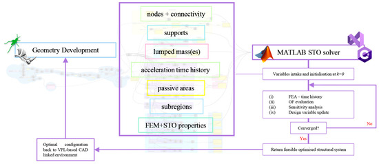
Figure 1.
VPL workflow and MATLAB-based STO tool’s connection.
3.1. User-Level Details
The plugin was developed in the C# programming language using the vs. Integrated Development Environment (IDE), with the MATLAB (v.2018b)-based code integrated into vs. as a .dll format. Initially, the user can create any desired geometry in the VPL environment and generate a mesh. The primary inputs of the plug-in are the coordinates of the nodes (Point List) and connectivity of the FE mesh (Data Tree). The subsequent inputs are the boundary conditions of the problem, which must be a Point List for which all Degrees Of Freedom (DOFs) are to be constrained, specifically translations in the X and Y directions. Subsequently, the coordinates of the nodes in which the concentrated masses are considered must be provided (Point List). This constitutes the minimum geometrical information required to formulate the STO problem.
The input data structure for the FEM problem comprises the following properties in this specific order: (i) OF, (ii) Simulation Time (T_max), (iii) Mass Magnitude (Mi), (iv) Young’s modulus (E), (v) Poisson’s ratio (v), (vi) Mass Density (ρ), (vii) Element Thickness (th), (viii) Rayleigh Damping (Ag), and (ix) Tag for Regular Meshes. The subsequent input is the ground acceleration applied to the STO problem, provided in .txt format with each row representing the acceleration for each time step (ti). Subsequently, all parameters for the optimisation formulation should be provided in the following order: (i) filter radius (rmin), (ii) VolFrac, (iii) symmetry axis, and (iv) maximum number of iterations. The local file path, where the STO problem results will be stored, is also required. Lastly, a Boolean parameter determines whether the optimisation procedure will commence (Toggle). At the base of the component, as shown in Figure 2, optional geometric inputs may be included to impose constraints on the final output. The input PassiveEl comprises a Data Tree of points that defines the FE to be retained with ρ = 1 (the density of these elements is considered solid). The subsequent inputs pertain to potential sub-region constraints that may be imposed to regulate the maximum member size of the optimised structures, as described by Sanders et al. (2018) [55] and Giraldo-Londoño and Paulino (2020) [56,57]. Based on the empirical number of distinct sub-regions into which the initial structure is divided, an equivalent number of data points must be provided. In the absence of sub-region specifications, the STO solver will proceed without considering of any passive areas and/or sub-regions (g). Finally, to visualise the optimised structure, it is necessary for the user to define the Thr, which delineates the boundary between void and solid FEs.
3.2. Developer-Level Details
The development and the execution of the plug-in was performed using an Intel Core i7-7800X CPU @ 3.50GHz and 16 GB RAM. The OS was Windows 10 Pro, version 22H2, while the software used were Matlab2018b, Rhino V6.5, and Visual Studio 2019. The initial process phase involved collecting all user inputs employing the GH SDK [58] and transforming them into C# objects. Consequently, a preprocessing step was necessary to appropriately format the collected data for utilisation in the MATLAB function. When extracting nodes from a GH file (.gh) containing mesh elements, it is common to encounter duplicated points. This redundancy arises from the mesh generation process, where nodes associated with multiple elements can share identical coordinates. Thus, to maintain an accurate representation of the geometry in designs featuring consequential FE, it is essential to identify and remove these duplicate nodes from the list. Next, the connectivity information is modified to transform a collection of point coordinates into a matrix. Each row of the matrix contains unique identifiers (IDs) of the nodes constituting each element. Subsequently, the Data Trees containing nodes and elements are converted into arrays, with each row containing a node ID or element belonging to the corresponding group of nodes or elements (e.g., support nodes and passive elements). Finally, before invoking the MATLAB function, MWNumericArray and MWArray are employed to convert all the data into a format compatible with the MATLAB platform.

Figure 2.
GH canvas—wired elements for the STO problem’s resolution and TO solution in Rhino3D Viewport Front Area.
As previously stated, the primary core of the dynamic STO solver is implemented in MATLAB [26], and additional preprocessing calculations must be performed in the same environment. Of particular significance is the requirement to arrange the nodes of the element connectivity in an anticlockwise order, as this information is retrieved from .gh, which does not guarantee this specific condition (necessary for FEA). All pre-processing calculations, in conjunction with the script that invokes the STO solver, are encapsulated within a function that receives GH component input. Subsequently, utilising the MATLAB Compiler SDK (Library Compiler), all requisite functions are wrapped into a .dll file that can be imported into the VS. Through this method, the primary MATLAB function is called from the C# script, which is compiled in a GH Assembly file, and the GH component is generated. (Figure 2). In order to execute the components in the VPL environment, both the .gh and .dll files must be inserted into the Library folder of the GH installation (Rhino→Grasshopper→File→Special Folder→Library), enabling it to function akin to any other GH add-on.
A complete demonstration of the user interaction within the developed GUI is illustrated in Figure 1 and Figure 2, showing the entire workflow—from geometry creation and FEM setup in the VPL environment to TO and visualisation in Rhino 3D. To ensure transparency and reproducibility, all Grasshopper definitions, MATLAB solver scripts, and resulting optimised geometries have been made openly available in the public GitHub repository linked to this research. The repository also includes a detailed README file describing each step of the process, from input preparation and solver execution to result post-processing and export in Rhino 3D.
3.3. Generation of the Initial Geometries of the Case Studies
Prior to executing the STO solver, the initial geometries were obtained through a parametric modelling workflow. The process was segmented into several phases, including the definition of the design domain that was modelled in the VPL environment—GH for Rhino (v.7). The initial geometry is defined through points, curves, or surfaces (Figure A1). The mesh may vary (structured or unstructured) in the two primary categories that represent the base test cases; however, the workflow logic remains consistent. The design domain is discretised through specific GH components with outputs organised in ordered lists; for the structured mesh, a quadrangular mesh system obtained through the Lunchbox add- will be adopted on [59], whilst for the unstructured mesh, a GH construction of a 2D Voronoi diagram will be employed.
Passive areas, i.e., regions that must maintain a density ρ = 1, are selected manually or through geometric criteria developed through VPL scripting. The passive elements are subsequently returned in the form of Data Trees, wherein each branch contains the list of linked points that are creating each passive FE (Figure A2).
Support points corresponding to constrained nodes, are identified and organised as separate inputs. In VPL, this process is accomplished through node coordinate selection components, which are subsequently filtered and converted into structured lists (Figure A3). The concentrated masses are determined on specific nodes through a coordinate ID system and mass magnitude assignment. By identifying the appropriate location for the lumped mass assignment, the specific coordinate for the application is retrieved from the total Point List derived from the mesh system. In Figure A4, the selection is based on the total point coordinates deconstruction such that the masses are situated at specific heights on the z-axis.
To ensure control over the material distribution within the design domain, Ω is divided into sub-regions. Each sub-region is defined as a distinct subset by dividing the total height of the building into equal parts, thus creating a series of sub-elements. The list of FEs belonging to each sub-region is subsequently organised in separate Data Trees containing the IDs of the individual FEs and the nodes belonging to them, thereby facilitating management during data transfer (Figure A5).
The close integration of VPL and MATLAB facilitates an automated workflow. Geometric data and boundary conditions are input into the GH environment (VPL) and organised into compatible matrices. Subsequently, the solver computes mass, damping, and stiffness matrices, solving the dynamic problem. The final density distribution map is returned to the .gh, where it can be visualised or exported with the “Bake” command into the CAD program.
3.4. Post-Processing and Export Features
After the optimisation process, the CAD-integrated framework (Rhino + GH V6.5 and later) provides post-processing functionalities to transform the density field into a clean, buildable geometry. The optimised density field is transmitted from MATLAB to Grasshopper as an indexed list of finite elements, where each index corresponds to a specific mesh element of the initial discretisation. This information is received by the Densities results output component (see Figure 2), which associates each element index with its corresponding density value.
A threshold parameter (Thr) is then applied within GH to distinguish solid and void regions. Elements whose density values exceed the threshold are identified as active members and extracted from the complete mesh from the initial density; this process isolates the subset of structural elements that define the final optimised layout.
Each selected element preserves its original nodal connectivity and geometric position, as imported from MATLAB, ensuring full consistency between the numerical model and the visualised mesh in Rhino 3D.
To enhance the readability of the optimised topology, edge detection and smoothing can be applied to the selected mesh. In practice, these operations can be implemented using native and plugin-based GH components such as Mesh Edges, Weaverbird Laplacian Smoothing, and Remesh, which remove irregularities and improve the visual continuity of the structure. Connectivity repair between adjacent elements can automatically be performed through the Join Meshes and Weld components, merging coincident vertices and eliminating small gaps along shared edges.
Finally, the refined mesh can be subdivided using the components such as Rhino’s QuadRemesh tools to improve the resolution of the final layout before export.
Then, the final mesh can be baked into Rhino 3D and exported to standard CAD formats (.3dm, .stl, .obj) or text-based files (.csv, .txt) for further analysis or fabrication. This integration ensures a continuous workflow from density-based optimisation to editable, fabrication-ready geometry, demonstrating the interoperability between the MATLAB solver and the visual programming interface.
In the next sections, several test cases are presented to assess the framework’s capability; specifically, two distinct geometries and mesh systems for the structural system of tall buildings are investigated under different dynamic loading conditions.
4. Numerical Case Studies
This section presents case studies on the dynamic STO application in tall buildings employing the developed VPL framework. All numerical examples are restricted to 2D plane-stress models, consistent with façade-like geometries on the XZ plane. Therefore, the current release is limited to two-dimensional meshes. The focus is minimising the square displacement at a target DOF, as outlined in Equation (1) for Single Degree of Freedom (SDOF) systems. In Multi-Degrees of Freedom (MDOFs), the OF minimises the sum of the square displacements of each DOF. The numerical test cases in Section 4.1 and Section 4.2 involve a tall building with a quadrangular base measuring 20 × 20 m and a height of 60 m. Various parameters and filters are varied during the analysis. The building’s façade is initially defined as a surface, then divided into regular quadrangular FEs using the Lunchbox© plug-in in GH. In this case, the surface is divided into 80 × 240 quad-panels, generating 19,200 FEs (Figure 3).
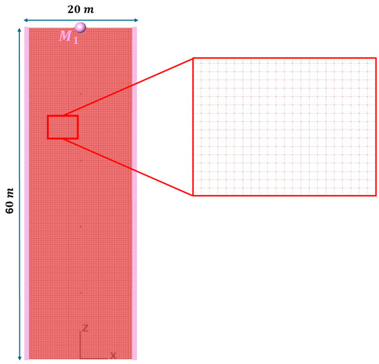
Figure 3.
Façade1, quad-mesh, 19,200 FEs.
This subdivision is empirically calibrated to ensure satisfactory mesh discretisation, yielding accurate results during the optimisation. Additionally, the filter radius size setting (rmin) is also taken into account. The rmin is applied after computing the elemental criterion to mitigate the occurrence of a checkerboard pattern in the optimised solution. This filter modifies the elemental criterion of a specific element by calculating a weighted average value within a specified neighbourhood. The user determines the rmin, which should exceed the size of the smallest FE to be effective (Figure 4). Adjusting the filter radius size enables control over the minimum size of the resulting features within the design domain [60], generally preventing compression-dominated regions from becoming overly thin.
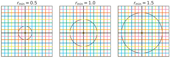
Figure 4.
Filter radius rmin representation with a single cell base = height, 0.25 × 0.25 cm.
Passive areas are incorporated into the model; these specific elements are designated as non-optimisable by the solver (see Figure 5). For convenience, the configuration shown in the following figure and in Figure 3 will be referred to as “Façade1” throughout the rest of the document.
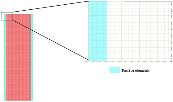
Figure 5.
Façade1: Passive areas definition and quad-mesh FE.
The building inter-storey is set at I = 3 m, so the tall building is hypothesised with a total of 20 floors. To simplify the problem, a single lumped mass Mi is initially considered on top of the building (Figure 3). The magnitude of M1 is defined considering the building footprint as follows:
where B represents the building footprint (m2).
Reliable values regarding the floor thickness Θ were considered according to Eurocode 2 as follows [61]:
This allows calculation of the slab volume S per each floor by considering the following building footprint B:
By assuming the concrete density as γcr = 2400 kg/m3, a single slab mass value ranges from 0.12 × 10⁶ kg to 0.288 × 10⁶ kg:
Considering γs = 100 kg/m3 for the steel reinforcement, the mass value to be added varies as [5000, 12,000] (kg). Therefore, the total mass of the single floor lies in the range [0.125 × 10⁶, 0.3 × 10⁶] (kg) (MassΘmin, MassΘmax).
Two different values for the lumped masses are considered in the numerical test cases, corresponding to Θmin and Θmax. Therefore, by fixing a total number of twenty floors, the total mass magnitudes for the case studies are calculated as and . Having considered four areas of influence, since the optimisation phase contemplates only the two-dimensional development, the mass magnitudes are and .
For all the subsequent case studies, the following parameters were settled as follows: (i) E = 210,000 MPa; (ii) ν = 0.3; (iii) ρ = 7800 kg/m3; (iv) th = 1 m; (v) Ag = [2, 2 × 10⁻⁶]; (vi) OF as in Equation (1); (vii) VolFrac = [0.3; 0.4]; (viii) rmin = [1]; (ix) Thr = 0.5; (x) Mi = [Mmin’, Mmax’]. The façade thickness does not correspond to the physical cladding thickness but represents an equivalent homogenised depth that accounts for the tributary contribution of mullions, spandrels, and secondary framing. For consistency, a reference value th = 1 m is adopted as a normalisation choice, ensuring proportional scaling of stiffness and mass per unit area.
While Section 4.1 and Section 4.2 focus on the application of the STO on the structured quad-mesh, Section 4.3 will analyse a special case of an unstructured mesh within a complex design domain. However, all the parameters listed above will remain unchanged. More information about the geometrical model is provided in the dedicated subsection.
4.1. Simple Harmonic Motion in Structured Mesh
In this subsection, the initial set of case studies focuses on applying SHM to evaluate the initial response of the VPL framework in a simplified scenario. In all dynamic simulations, the excitation is introduced as a ground motion imposed at the base of the façade domain. In the harmonic case, the ground acceleration is defined as a sinusoidal input with angular frequency ω. In the earthquake cases, the excitation corresponds to recorded accelerograms applied as base accelerations at the support nodes.
Although only single-excitation results are reported herein for clarity, the proposed framework inherently supports multiple dynamic load cases. Owing to the linear nature of the equilibrium equation, different excitation windows or SHM frequencies can be superimposed to perform multi-load analyses, allowing robustness assessments without modifying the optimisation algorithm.
In this context, the imposed base acceleration for the harmonic case is defined as follows:
where the peak acceleration is 5 m/s2, T_max is capped at 4.8 s with 80 time-steps, and the angular frequency is ω = 2.5π rad/s (Figure 6).
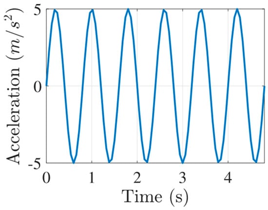
Figure 6.
SHM application—fi in the dynamic problem.
4.1.1. Case Study No.1 Imposing SDOF, 1 g, SHM
The first results are obtained solving the minimisation problem in Equation (1), by imposing one sub-region g1 as constraint in Façade1 in the XZ plane under SHM (Figure 6). The fixed support points are located at the base (Figure 7). Two different tests were carried out by varying M1[min’, max’] while maintaining constant the VolFrac = 0.3 for the sub-region g1 (no sub-region is developed in the GH workflow).
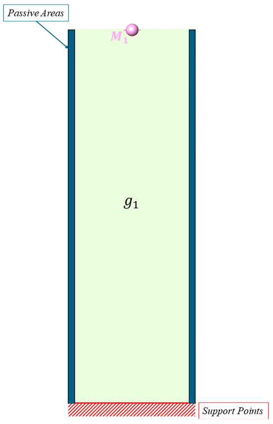
Figure 7.
Façade1 definition, single concentrated mass M1, single sub-region g1.
Figure 8 displays the evolution of the bracing system developed by the VPL solver using a unified design domain. The complete optimisation of Test Case 1 required approximately 15 min on a standard workstation (Intel i7, 32 GB RAM), with a peak memory usage of about 2.6 GB.
In this scenario, M1 is set as for the left configuration (Figure 8a) and for the right configuration (Figure 8b). Applying SHM excitation, the results revealed a significant dependence of bracing system topology on M1; the optimised design demonstrated for M1,min′ a uniform diagonal bracing pattern, while for M1,max′ a denser bracing structure to counteract increased inertial forces. Despite the design codes not providing a direct horizontal deflection limit, recent research has demonstrated that most of the δmax for tall buildings varies in the range of values [15,62]. In our case, the optimised designs demonstrated for M1,min′ a maximum horizontal displacement located at the position of the targeted DOF equal to δmax = 0.031 m, and for M1,max′ a larger displacement such as δmax = 0.082 m. The results show a realistic outcome in terms of practical application, since δmax for M1,max′ is slightly smaller than . The δmax increased with mass magnitude, confirming the solver’s ability to adjust material distribution based on dynamic demand. The rmin helped smooth out density variations, preventing unrealistic checkerboarding effects in the optimised topology. The test case confirms that larger mass magnitudes require denser bracing, particularly in the lower regions of the structure.

Figure 8.
Façade1, dynamic STO results, SDOF, 1 g; δmax over time and final configuration for (a) M1min′, (b) M1max′.
4.1.2. Case Study No.2 Imposing SDOF, 5g, SHM
The second analysis carried out on Façade1 consists of applying five distinct sub-regions denoted as g[1, 5] (Figure 9). Each sub-region is evaluated in the STO problem separately, considering the value VolFrac = 0.4. Support points and passive areas are equal to Test No.1, as indicated in the following picture.
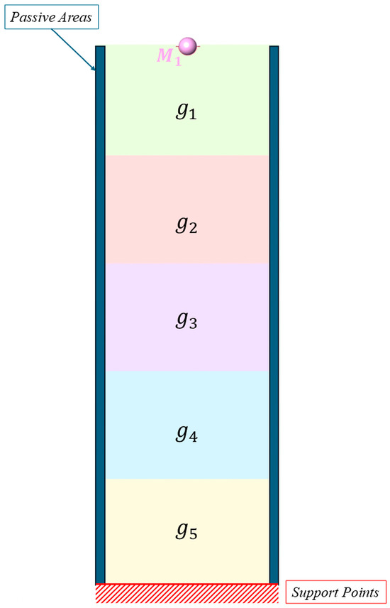
Figure 9.
Façade1, inclusion of 5 sub-regions g[1, 5]; SDOF, M1 variable.
After applying the SHM in Equation (23) and illustrated in Figure 6, by minimising the square displacement located at M1, the following results were observed. Figure 10 illustrates the evolution of the bracing system post-optimisation relating to a value of M1 equal to (Figure 10a) and to (Figure 10b) based on the above-described calculations involving Eurocode 2. The results show the maximum lateral displacement obtained by applying SHM as δmax = 0.031 m with M1,min′ and δmax = 0.068 m by applying M1,max′. The introduction of five sub-regions resulted in a more stable, evenly distributed bracing layout compared to the single-region case. As mass increased, the material remained concentrated along the main lateral force transmission paths, confirming the stability and robustness of the STO solver. The results highlight the importance of introducing a filtering scheme that simultaneously imposes a target length scale in both solid and void phases, as they ensure better material allocation across different load conditions [63]. In this scenario can be noticed the sensitivity of the system to the VolFrac parameter. By observing Case Study No.1 in Figure 8, the change in the lateral bracing system topology clearly emerges as the VolFrac increases, despite rmin not varying in both cases. The δmax in M1max′ was reduced due to the increased material retention across the sub-regions resulting from the imposition of a higher VolFrac value. However, considering the actual results pertaining to δmax and the general indication provided by Smith, R. (2011) [62], achieving such a low lateral displacement value is not necessary. Consequently, in the subsequent case studies applying SHM, VolFrac = 0.3 is utilised.
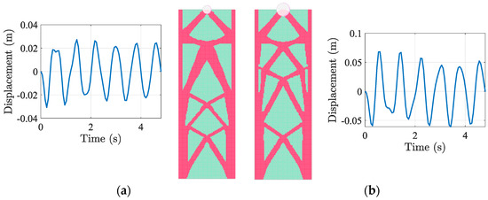
Figure 10.
Façade1, dynamic STO results, SDOF, 5 g; δmax over time and final configuration for (a) M1min′, (b) M1max′.
4.1.3. Case Study No. 3 Imposing MDOFs, 1 g, SHM
The third case study extends the SDOF case by distributing five concentrated masses at different heights and analysing how the material distribution adapts. The lumped massed M[1, 5] are located at specific coordinates along the height of the building, as follows {x, y, z}: M5 = {0, 0, 12}; M4 = {0, 0, 24}; M3 = {0, 0, 36}; M2 = {0, 0, 48}; M1 = {0, 0, 60} (Figure 11). The different applied mass magnitudes are derived by equally subdividing the total magnitude defined as , such as . Also in this case, the STO problem is addressed by applying dynamic forces in the form of SHM while VolFrac = 0.3. In order to simplify the problem, a single region is contemplated (g = 1). Since it is considered an MDOF system, it is minimised as the sum of square displacements at the targeted DOFs.
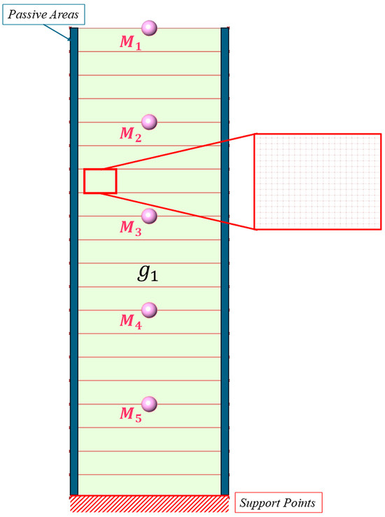
Figure 11.
Façade1, Numerical Test Case No. 3. MDOFs, 1 g.
The findings in Figure 12 indicate that including the five lumped masses M[1, 5] brings about a more even distribution of diagonal members throughout the height, notably linked to their location. In this case, at the structure’s tip is obtained δmax = 0.062 m by applying M[1, 5]min′, while applying M[1, 5]max′ leads to δmax = 0.205 m. The results show that the STO solver distributed diagonal bracing evenly across the entire height, reflecting the contributions of multiple mass locations. Increased masses resulted in thicker diagonal members near mid-height, as inertia forces accumulated in the middle levels. In comparison with Case Study No. 1, the presence of MDOFs led to a more uniformly distributed bracing system in the height of Façade1. The introduction of MDOFs simulates a more realistic representation of the mass distribution within a tall building. The higher value of δmax, compared to a SDOF system, resulted in improved accuracy of the maximum lateral displacement, particularly evident in the M[1, 5]max′ application, falling within the suggested range [62], such as . These results demonstrate strong alignment with real-world bracing strategies, highlighting the significance of incorporating MDOFs compared to the simplified assumption made in SDOF adoption.
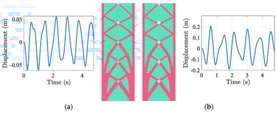
Figure 12.
Façade1, dynamic STO results, MDOFs, 1 g. δmax over time, final configuration for (a) M[1, 5]min′, (b) M[1, 5]max′.
4.1.4. Case Study No.4 Imposing MDOFs, 5 g, SHM
The following numerical test for applying SHM in the STO problem was carried out on Façade1 by applying five simplifications of sub-regions within the total design domain Ω, setting the parameter related to g = 5. In this scenario, we maintain VolFrac = 0.3 and rmin = 1, while applying five lumped masses M[1, 5] to create an MDOF system, as shown in the accompanying illustrative image (Figure 13).
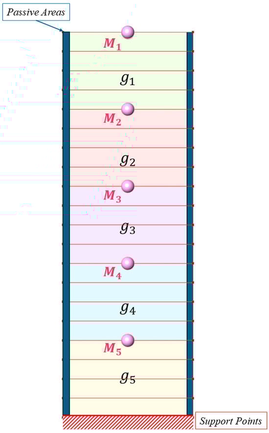
Figure 13.
Façade1, MDOFs, 5 g.
The outcomes in Figure 14 indicate that the introduction of g[1,…,5] results in a uniform distribution of the material within each imposed sub-region. This contrasts with the observations from the previous Case Study No. 3, where the material percentage defined by the VolFrac parameter is predominantly located at the base of the tall building. The maximum horizontal displacement proportionally follows the applied magnitude as δmax = 0.071 m in M[1, 5]min′, while δmax = 0.255 m in M[1, 5]max′. Significant observations from the latest results can be made, noting that the bracing members became more uniform in thickness, demonstrating that multiple sub-regions enhance material allocation efficiency. Consequently, δmax is increased compared to Case Study No. 3, indicating that subdividing the design domain into sub-regions led to equal material distribution within the lower and upper sections. Considering that for M[1, 5]max′, , the outcome still meets the general range of lateral displacements found in the real data concerning tall buildings. Thus, combining MDOFs and multiple sub-regions not only results in a well-distributed bracing system that provides enhanced resistance against lateral forces while maintaining material efficiency, but also can assist designers involved in the architectural, engineering, and construction (AEC) industry in the decision-making process, offering the possibility to consider the same material distribution within the sub-region to meet constructability criteria using fewer different cross-sections to produce bracing systems.
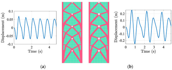
Figure 14.
Façade1, STO results, SHM, MDOFs, 5 g. δmax over time and final configuration for (a) M[1, 5]min′, (b) M[1, 5]max′.
4.2. Real Earthquake Data in STO
In this study, appropriate recorded earthquake data from ground motion time histories were utilised to simulate seismic excitations for optimising structural dynamic design, with the objective of enhancing structural resilience in highly seismic regions. Two distinct ground motion accelerations () were employed, namely the L’Aquila earthquake (Italy, 2009) and the Athens earthquake (Greece, 1999). In the subsequent test cases, the same design domain configuration as Façade1 is adopted; the accelerogram is integrated into the solution for the earthquake response spectrum, while the parameters E, v, ρ, th, Ag, rmin, and Thr remain consistent across both the SHM and earthquake simulations.
4.2.1. Case Study No.5—L’Aquila Earthquake
The first test deals with the L’Aquila earthquake, which occurred in Italy in 2009. The recording source of the event and the characteristics of the earthquake are herein summarised: Station Code: AQK; source ITACA ID IT-2009-0009; Processing manual [64], Event time: 6 April 2009 01:32:40 [65]. In order to reduce the computational cost, the time interval [30.4, 42.9] (s) was chosen for a total duration of T_max = 12.5 (s), while the discretisation referring to the time step is equal to ti = 0.01 (s) (Figure 15).
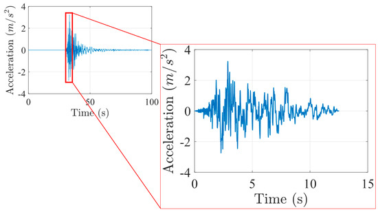
Figure 15.
L’Aquila Earthquake (2009); zoom on time interval [30.4, 42.9] (s).
To compare the results by applying the same external excitation, two primary test cases were developed by varying the number of lumped masses applied and their magnitude, the VolFrac, and the number of sub-regions. Specifically, the first test case is initially simplified by applying a single lumped mass M1 = Mmin′ while adopting five sub-regions (see Figure 9) with VolFrac = 0.4. Subsequently, another configuration was created with the incorporation of five DOFs (M[1, 5]) into Façade1 within the VPL environment; in this instance, the design domain was treated as a single region, denoted as g = 1 (see Figure 11) while the magnitude of M[1, 5] = Mmax′ and VolFrac = 0.3. The comparative results presented in Figure 16 illustrate the optimised structure under the seismic activity that occurred in L’Aquila in 2009, adopting different parameter settings.
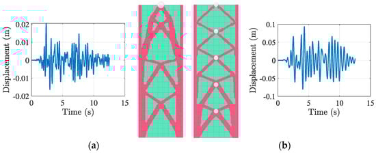
Figure 16.
Results of dynamic STO, L’Aquila Earthquake (2009). (a) SDOF, M1 = Mmin′, VolFrac = 0.4, 5 g, (b) (5) MDOFs, M[1, 5] = Mmax′, VolFrac = 0.3, 1 g.
The upper figure, illustrating the results for the two distinct test cases subjected to identical external forces, demonstrates the solver’s efficacy in developing bracing-like material patterns in response to authentic seismic motions, thus indicating practical applicability in the field of seismic engineering. The δmax observed during the optimisation process for the SDOF (a) was δmax = 0.020 m, while the MDOF system (b) recorded a higher maximum displacement of δmax = 0.093 m.
In configuration (a), the material distribution in the façade deviates from the typical expected outcome, particularly when compared to (b). This discrepancy arises from the contrast between the realistic seismic force and the unlikely simplified representation of the tall building as a single lumped mass system with a total height of 60 m. Moreover, the introduction of multiple sub-regions resulted in a more uniform material distribution along the structure’s height, without differentiating the impact of the seismic action at different heights of the building. Extending the L’Aquila test to incorporate the MDOF system yielded several notable findings: lateral bracing became evenly distributed, reducing stress concentrations near mass points, and diagonal bracing patterns emerged predominantly in the lower half of the structure. The observed differences in material distribution in (b) are attributed to the single sub-region application, demonstrating the solver’s adaptability in the absence of specific constraints; additionally, the larger displacement can be linked to the higher total mass and lower VolFrac. The optimised structures demonstrated improved resilience against earthquake-induced displacements, since the δmax obtained remained within anticipated seismic performance thresholds. Both designs demonstrate adaptation to the earthquake loading, with diagonal bracing patterns emerging to resist lateral forces.
4.2.2. Case Study No. 6—Athens Earthquake
With the aim of further investigating the impact of significant seismic ground motions on the previous geometry, the case of the earthquake that occurred in Athens, Greece, on 7 September 1999, was also examined. Despite its moderate magnitude and the low seismic risk of the corresponding zone, the earthquake caused severe damage [66]. In this instance, to reduce computational cost, the time interval [2.00, 7.00] (s) was chosen for a total duration of T_max = 5.00 (s) (Figure 17). The discretisation referring to the time step is equal to ti = 0.01 (s) [67].
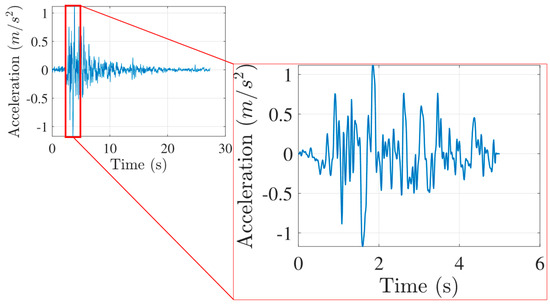
Figure 17.
Athens Earthquake (1999); zoom on time interval [2, 7] (s).
As for the previous case study, two comparative applications were developed. The set of results depicted in Figure 18 pertains to the MDOF system with M[1, 5] = Mmin′, VolFrac = 0.3, and rmin = 1. Specifically, configuration (a) focuses on a single region (g = 1) and relates to Façade1 illustrated in Figure 11, while in (b) the results refer to the application of five different sub-regions, i.e., g = 5 (see Figure 13).
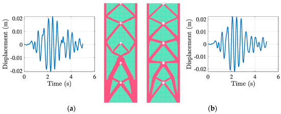
Figure 18.
Results of Dynamic STO, Athens Earthquake (1999). MDOFs, M[1–5] = Mmin′, VolFrac = 0.3. (a) 1 g. (b) 5 g.
In the left configuration (Figure 18a), δmax = 0.021 m was recorded on the x-axis. The results also indicate that diagonal members are distributed with increasing thickness progressing from the apex to the base of the tower due to the presence of a single sub-region. In the right configuration (Figure 18b), with the application of multiple sub-regions, the optimised bracing was uniformly distributed, preventing localised stress accumulation. δmax = 0.022 m remained stable compared to (a) due to the same mass magnitude application, demonstrating further refinement in material utilisation. Compared to the MDOF L’Aquila earthquake results (Figure 16b), the topology (a) displayed alterations due to variations in frequency content. The solver demonstrated effective adaptation to various earthquake stimuli while balancing material usage and displacement control, highlighting its practical applicability across different seismic regions.
4.3. SHM in Unstructured Mesh
In this subsection, the proposed VPL framework was used to tackle the dynamic STO problem for irregular geometries. This updated application enables the creation of geometry within a complex design domain, which includes various mesh cell geometries, such as Voronoi tessellations. To assess the VPL framework effectiveness with irregular geometries, an initial configuration of the design domain Ω was set up. This configuration features a circular structure on the XZ plane, supported at its base. The base structure has a height h = 90 m and a base width b = 20 m. The mesh is discretised into Voronoi cells directly created in the VPL-CAD linked environment based on empirical determination, in order to ensure accurate evaluation while maintaining computational efficiency. A total of 7984 Voronoi elements were utilised in the discretisation (Figure 19); for clarity, we shall refer to the specific geometry characterised by unstructured mesh as “Façade2”.
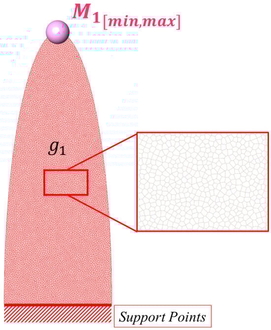
Figure 19.
Unstructured Mesh Development—Voronoi tessellation and lumped mass variation.
The following tests evaluated the behaviour of the VPL—STO solver for a tall building subjected to SHM excitation following the external force characteristics listed in Section 4.1 (Figure 6). A concentrated single lumped mass with variable magnitudes given by M1min′ and M1max′ is considered. In this particular scenario, no passive areas and sub-regions (g = 1) were designated to assess the outcome of the STO with minimal constraints. The minimum filter radius size was established as rmin = 1.
In Figure 20 are reported the results obtained by imposing Equation (1) and employing the produced add-on in VPL, according to Section 3; specifically, in the STO setting, a pattern of variable conditions imposed is listed as follows: (a) VolFrac = 0.3, M1min′; (b) VolFrac = 0.3, M1max′; (c) VolFrac = 0.4, M1min′; (d) VolFrac = 0.4, M1max′.
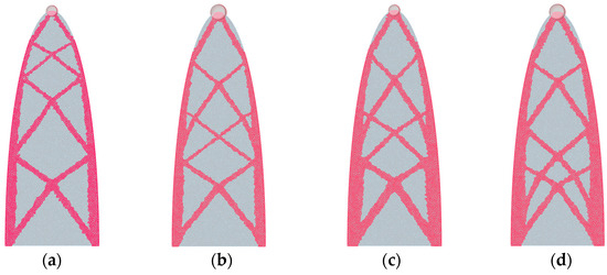
Figure 20.
Post-STO Voronoi tessellation. VolFrac = 0.3 (a) M1,min′, (b) M1,max′; VolFrac = 0.4 (c) M1,min′, (d) M1,max′.
As variations in VolFrac and mass magnitude occur, distinct lateral deflection values and topological characteristics emerge in the two systems under consideration. The diagrams in Figure 21 illustrate, in both instances, the displacement trend as a function of time. Specifically, in Figure 20a, δmax = 0.041 m is obtained, while in Figure 20b δmax = 0.107 m is recorded. Similarly, by setting VolFrac = 0.4 in Figure 20c,d, different results concerning both the topological configuration and the lateral displacement values are obtained, as demonstrated from (c) in which δmax = 0.033 m and in (d) where δmax = 0.068.
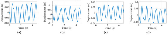
Figure 21.
Post-STO δmax. VolFrac = 0.3 (a) M1,min′, (b) M1,max′; VolFrac = 0.4 (c) M1,min′, (d) M1,max′.
The observed δmax in both instances correlates with the mass magnitude variation, as well as the modifications in material allocation with additional bracing systems incorporated as the mass increases, thereby facilitating the transfer of inertial forces to the supports. In addition to the mass magnitude variation, the sensitivity to the VolFrac is also examined. In the case of the unstructured mesh, the structure exhibits a response to the filter variation, indicating that the data transmission from VPL to the STO solver is comprehensive. The bracing structure adapted to the irregular mesh and design domain, demonstrating flexibility in accommodating non-standard geometries. The material distribution remained stable despite the complex Voronoi tessellation, confirming the solver’s connection robustness. The displacement values results aligned well with structured-mesh cases, ensuring accuracy regardless of meshing strategy.
5. Conclusions and Discussion
This research advances STO in the context of earthquake engineering, demonstrating an integrated computational framework that enhances structural resilience under dynamic loading. By integrating time history ground motion data into the STO framework, a VPL tool within GH for Rhino3D was developed, enabling design of structures that are material efficient and highly resistant to seismic forces. This integration addresses the need for structures to withstand complex forces generated by earthquakes, ensuring optimisation techniques are directly applicable to real-world engineering problems. A key achievement is the seamless connection between the VPL-CAD linked tools and MATLAB-based programming. The integration within a VPL environment enhances STO accessibility for engineers and architects, allowing users to define geometries, set optimisation constraints, and visualise results within a single workflow. By embedding numerical optimisation techniques into the VPL environment, the approach reduces the gap between analysis and design, enabling an iterative process that ensures optimal structural performance under dynamic loads.
The numerical test cases confirm that material distribution, mass magnitude, and sub-region constraints significantly influence bracing topology, highlighting the importance of considering concentrated mass locations and dynamic excitation characteristics. The integrated VPL framework effectively adapts to varying conditions, redistributing material in response to seismic and harmonic loading, thereby ensuring optimal stiffness and structural efficiency. The application of real earthquake data, including L’Aquila (2009) and Athens (1999) ground motion records, validates the approach’s ability to minimise the displacements at a target DOF while maintaining efficient material use, demonstrating its potential for compliance with modern seismic engineering standards. The observed variations in bracing topologies between the two earthquakes emphasise the need for a data-driven, site-specific approach to seismic-resistant design, as different frequency contents and intensities demand tailored optimisation solutions. Furthermore, the implementation of STO on an unstructured Voronoi tessellation extends the method’s versatility, proving its capability to handle complex, irregular geometries while maintaining structural stability. The ability to optimise both structured and unstructured mesh systems ensures that engineers and designers have the flexibility to explore innovative structural forms while maintaining high efficiency and safety employing a CAD-friendly environment.
This study confirms that integrating STO within a CAD-based VPL enhances accessibility, efficiency, and practicality. The combination of parametric design tools, numerical optimisation techniques, and real-time visualisation allows for rapid generation and refinement of optimised structural layouts, ensuring engineering accuracy without extensive manual intervention. The research highlights the value of integrating coding-based methodologies with CAD platforms, transforming STO into a powerful, practical solution for real-world engineering challenges. Future research will refine optimisation algorithms to enhance computational efficiency, especially for large-scale and three-dimensional structures. Studies will extend the methodology to multi-hazard scenarios, incorporating seismic, wind, and impact loads for more resilient designs. Expanding the problem library to include diverse structural typologies, materials, and load conditions would further validate the solver’s efficacy in various engineering contexts. Enhancing VPL-CAD integration and expanding STO capabilities will help develop safer, more resilient, and sustainable infrastructure to withstand extreme dynamic events, advancing seismic-resistant structural design.
Author Contributions
Conceptualisation: L.S., S.S.; Data curation: L.S.; Formal analysis and investigation: L.S., S.S.; Funding acquisition: L.S.; Methodology: L.S., S.S.; Project administration: L.S.; Resources: L.S., S.S.; Software: L.S., S.S.; Supervision: A.F.; Validation and Visualisation: L.S., S.S.; Writing—original draft preparation: L.S.; Writing—review and editing: L.S. All authors have read and agreed to the published version of the manuscript.
Funding
Dr. Laura Sardone carried out this study within the RETURN Extended Partnership and received funding from the European Union Next-GenerationEU (National Recovery and Resilience Plan—NRRP, Mission 4, Component 2, Investment 1.3—D.D. 1243 2/8/2022, PE0000005). Dr. Alessandra Fiore acknowledges the research projects: PRIN PNRR 2022 “Artificial Intelligence for ENVIronmental impact minimisation of SEismic Retrofitting of Structures (AI-ENVISERS)”; PRIN 2022 “Digitalised life-cycle management of historic bridges by an integrated monitoring and modelling CDE platform—HBridgeIM (Historic Bridge Information Modelling)” (2022744YM9).
Data Availability Statement
The data are openly accessible in the following GitHub repository: https://github.com/stsotirop/VPL_DTO/tree/main (accessed on 28 October 2025). The verifiability and replicability of the results are ensured through the open-access publication of the case studies presented in this paper, as well as the software for the Visual Programming Language (VPL) and the associated environment (Grasshopper® for Rhinoceros 3D). The implementation requires licensed (or trial) versions of Rhinoceros 3D (v6.0 or later) with Grasshopper, and MATLAB2018b. The framework has been tested on Windows 10; compatibility with other operating systems has not yet been verified. For installation, copy the Grasshopper definition (.gh) and the compiled plugin (.dll) into the Grasshopper Libraries folder; the new components will be automatically loaded at Rhino startup. The repository also provides a README with detailed setup and execution instructions, enabling step-by-step reproduction of the results.
Conflicts of Interest
All authors certify that they have no affiliations with or involvement in any organisation or entity with any financial interest or non-financial interest in the subject matter or materials discussed in this manuscript.
Abbreviations
The following abbreviations are used in this manuscript:
| STO | Structural Topology Optimisation |
| CAD | Computer-Aided Design |
| VPL | Visual Programming Language |
| GUI | Graphical User Interface |
| DOF | Degrees of Freedom |
| SDOF | Single Degree Of Freedom |
| SO | Structural Optimisation |
| TO | Topology Optimisation |
| GH | Grasshopper |
| AEC | Architecture, Engineering, and Construction |
| SIMP | Solid Isotropic Material Penalisation |
| CAE | Computer-Aided Engineering |
| DDM | Direct Differentiation Methods |
| AVM | Adjoint Variable Methods |
| MDOF | Multi-Degree Of Freedom |
| OF | Objective Function |
| RAMP | Rational Approximation of Material Properties |
| SHM | Simple Harmonic Motion |
| FEM | Finite Element Model |
Appendix A
Figure A1, Figure A2, Figure A3, Figure A4 and Figure A5 show the step-by-step Grasshopper workflow used to generate the façade models based on a quadrangular mesh system. These screenshots complement the GitHub repository and are provided to guide readers through the implementation.

Figure A1.
Geometry development in VPL—Tall Building 20 × 60 (m).

Figure A2.
Passive areas selection in GH canvas.

Figure A3.
Support points in GH canvas.

Figure A4.
Lumped masses in GH canvas.

Figure A5.
Sub-regions definition in GH canvas.
References
- Duarte, L.S.; Celes, W.; Pereira, A.; Menezes, I.F.M. PolyTop++: An efficient alternative for serial and parallel topology optimization on CPUs & GPUs. Struct. Multidiscip. Optim. 2015, 52, 845–859. [Google Scholar]
- Mukherjee, S.; Breitkopf, P.; Zhang, W.; Dutta, S.; Xiao, M.; Lu, D.; Raghavan, B. Accelerating Large-scale Topology Optimization: State-of-the-Art and Challenges. Arch. Comput. Methods Eng. 2021, 28, 4549–4571. [Google Scholar] [CrossRef]
- Bendsøe, M.P.; Kikuchi, N. Generating optimal topologies in structural design using a homogenization method. Comput. Methods Appl. Mech. Eng. 1988, 71, 197–224. [Google Scholar] [CrossRef]
- Zhang, J.; Sato, Y.; Yanagimoto, J. Homogenization-based topology optimization integrated with elastically isotropic lattices for additive manufacturing of ultralight and ultrastiff structures. CIRP Ann. 2021, 70, 111–114. [Google Scholar] [CrossRef]
- Altair. Altair® OptiStruct®. Available online: https://altair.com/optistruct/ (accessed on 15 January 2025).
- Yang, R.-J.; Chahande, A.I. Automotive applications of topology optimization. Struct. Optim. 1995, 9, 245–249. [Google Scholar] [CrossRef]
- Abualigah, L.; Diabat, A. A comprehensive survey of the Grasshopper optimization algorithm: Results, variants, and applications. Neural Comput. Appl. 2020, 32, 15533–15556. [Google Scholar] [CrossRef]
- CREATIVE MUTATION. Millipede. Available online: https://www.creativemutation.com/millipede (accessed on 14 January 2025).
- Sigmund, O. A 99 line topology optimization code written in Matlab. Struct. Multidiscip. Optim. 2001, 21, 120–127. [Google Scholar] [CrossRef]
- Zhou, Q.; Shen, W.; Wang, J.; Zhou, Y.; Xie, Y. Ameba: A new topology optimization tool for architectural design. In Proceedings of the IASS Symposium 2018, Creativity in Structural Design, Boston, MA, USA, 16–20 July 2018. [Google Scholar]
- Aage, N.; Nobel-Jørgensen, M.; Andreasen, C.; Sigmund, O. Interactive topology optimization on hand-held devices. Struct. Multidiscip. Optim. 2013, 47, 1–6. [Google Scholar] [CrossRef]
- Białkowski, S. Topology Optimisation Influence on Architectural Design Process—Enhancing Form Finding Routine by tOpos Toolset utilisation. In Proceedings of the eCAADe 2018, Lodz, Poland, 17–21 September 2018. [Google Scholar]
- He, L.; Li, Q.; Gilbert, M.; Shepherd, P.; Rankine, C.; Pritchard, T.; Reale, V. Optimization-driven conceptual design of truss structures in a parametric modelling environment. Structures 2022, 37, 469–482. [Google Scholar] [CrossRef]
- Selmı, M.; İlerisoy, Z.Y. A Comparative Study of Different Grasshopper Plugins for Topology Optimization in Architectural Design. Gazi Univ. J. Sci. Part B Art Humanit. Des. Plan. 2022, 10, 323–334. [Google Scholar]
- Stromberg, L.L.; Beghini, A.; Baker, W.F.; Paulino, G.H. Topology optimization for braced frames: Combining continuum and beam/column elements. Eng. Struct. 2012, 37, 106–124. [Google Scholar] [CrossRef]
- Sotiropoulos, S.; Lagaros, N.D. A two-stage structural optimization-based design procedure of structural systems. Struct. Des. Tall Spec. Build. 2022, 31, e1909. [Google Scholar] [CrossRef]
- Andreassen, E.; Clausen, A.; Schevenels, M.; Lazarov, B.S.; Sigmund, O. Efficient topology optimization in MATLAB using 88 lines of code. Struct. Multidiscip. Optim. 2011, 43, 1–16. [Google Scholar] [CrossRef]
- Talischi, C.; Paulino, G.; Pereira, A.; Menezes, I. PolyTop: A Matlab implementation of a general topology optimization framework using unstructured polygonal finite element meshes. Struct. Multidiscip. Optim. 2012, 45, 329–357. [Google Scholar] [CrossRef]
- Min, S.; Kikuchi, N.; Park, Y.C.; Kim, S.; Chang, S. Optimal topology design of structures under dynamic loads. Struct. Optim. 1999, 17, 208–218. [Google Scholar] [CrossRef]
- Bendsøe, M.; Sigmund, O. Topology Optimization: Theory, Methods and Applications; Springer: Berlin/Heidelberg, Germany, 2004. [Google Scholar]
- Kang, B.-S.; Park, G.-J.; Arora, J.S. A review of optimization of structures subjected to transient loads. Struct. Multidiscip. Optim. 2006, 31, 81–95. [Google Scholar] [CrossRef]
- Fleury, C.; Braibant, V. Structural optimization: A new dual method using mixed variables. Numer. Methods Eng. 1986, 23, 409–428. [Google Scholar] [CrossRef]
- Dennis, J.E.; Schnabel, R.B. Numerical Methods for Unconstrained Optimization and Nonlinear Equations; SIAM: Philadelphia, PA, USA, 1996. [Google Scholar]
- Byrd, R.H.; Nocedal, J.; Yuan, Y.-X. Global Convergence of a Cass of Quasi-Newton Methods on Convex Problems. SIAM J. Numer. Anal. 1987, 24, 1171–1190. [Google Scholar] [CrossRef]
- Yoon, G.H. Structural topology optimization for frequency response problem using model reduction schemes. Comput. Methods Appl. Mech. Eng. 2010, 199, 1744–1763. [Google Scholar] [CrossRef]
- Giraldo-Londoño, O.; Paulino, G.H. PolyDyna: A Matlab implementation for topology optimization of structures subjected to dynamic loads. Struct. Multidiscip. Optim. 2021, 64, 957–990. [Google Scholar] [CrossRef]
- Filipov, E.T.; Chun, J.; Paulino, G.H.; Song, J. Polygonal multiresolution topology optimization (PolyMTOP) for structural dynamics. Struct. Multidiscip. Optim. 2016, 53, 673–694. [Google Scholar] [CrossRef]
- Martin, A.; Deierlein, G.G. Structural Topology Optimization of Tall Buildings for Dynamic Seismic Excitation Using Modal Decomposition. Eng. Struct. 2020, 216, 110717. [Google Scholar] [CrossRef]
- Jin, F.; Yang, Y.; Xiao, Z.; Gao, B.; Lou, H. Shear wall layout optimization of multi-tower buildings based on conceptual design and extended evolutionary structural optimization method. Eng. Optim. 2023, 56, 486–505. [Google Scholar] [CrossRef]
- Du, Y.; Li, H.; Luo, Z.; Tian, Q. Topological design optimization of lattice structures to maximize shear stiffness. Adv. Eng. Softw. 2017, 112, 211–221. [Google Scholar] [CrossRef]
- Wang, B.; Cheng, G. Design of cellular structures for optimum efficiency of heat dissipation. Struct. Multidiscip. Optim. 2005, 30, 447–458. [Google Scholar] [CrossRef]
- Chopra, A.K. Dynamics of Structures: Theory and Applications to Earthquake Engineering, 4th illustrated ed.; Prentice Hall: Upper Saddle River, NJ, USA, 2012. [Google Scholar]
- Clough, R.; Penzien, J. Dynamics of Structures, 2nd ed.; McGraw-Hill: New York, NY, USA, 1993. [Google Scholar]
- Wilson, E.L. Three-Dimensional Static and Dynamic Analysis of Structures: A Physical Approach With Emphasis on Earthquake Engineering, 3rd ed.; Computers and Structures, Inc.: Berkeley, CA, USA, 2002. [Google Scholar]
- Rayleigh, J.W.S. The Theory of Sound; Macmillan: London, UK, 1877. [Google Scholar]
- Craig, R.R., Jr.; Kurdila, A.J. Fundamentals of Structural Dynamics, 2nd ed.; John Wiley & Sons: Hoboken, NY, USA, 2006. [Google Scholar]
- Jog, C.S. Topology design of structures subjected to periodic loading. J. Sound Vib. 2022, 253, 687–709. [Google Scholar] [CrossRef]
- Hilber, H.M.; Hughes, T.J.; Taylor, R.L. Improved numerical dissipation for time integration algorithms in structural dynamics. Earthq. Eng. Struct. Dyn. 1977, 5, 283–292. [Google Scholar] [CrossRef]
- Newmark, N. A method of computation for structural dynamics. J. Eng. Mech. Div. 1959, 85, 67–94. [Google Scholar] [CrossRef]
- Li, X.D.; Wiberg, N.-E. Structural Dynamic Analysis by a Time-Discontinuous Galerkin Finite Element Method. Numer. Methods Eng. 1996, 39, 2131–2152. [Google Scholar] [CrossRef]
- Herrero-Pérez, D.; Picó-Vicente, S.G.; Martínez-Barberá, H. Efficient distributed approach for density-based topology optimization using coarsening and h-refinement. Comput. Struct. 2022, 265, 106770. [Google Scholar] [CrossRef]
- Wang, Y.; Kang, Z.; He, Q. Adaptive topology optimization with independent error control for separated displacement and density fields. Comput. Struct. 2014, 135, 50–61. [Google Scholar] [CrossRef]
- de Troya, M.A.S.; Tortorelli, D.A. Adaptive mesh refinement in stress-constrained topology optimization. Struct. Multidiscip. Optim. 2018, 58, 2369–2386. [Google Scholar] [CrossRef]
- Stolpe, M.; Svanberg, K. An alternative interpolation scheme for minimum compliance optimization. Struct. Multidiscip. Optim. 2001, 22, 116–124. [Google Scholar] [CrossRef]
- Sui, Y.; Peng, X. Chapter 1—Exordium. In Modelling, Solving and Application for Topology Optimization of Continuum Structures: ICM Method Based on Step Function; Butterworth-Heinemann: Oxford, UK, 2018; pp. 1–36. [Google Scholar]
- Wang, F.; Lazarov, B.; Sigmund, O. On projection methods, convergence and robust formulations in topology optimization. Struct. Multidiscip. Optim. 2011, 43, 767–784. [Google Scholar] [CrossRef]
- Wadbro, E.; Hägg, L. On quasi-arithmetic mean based filters and their fast evaluation for large-scale topology optimization. Struct. Multidiscip. Optim. 2015, 52, 879–888. [Google Scholar] [CrossRef]
- Li, L.; Khandelwal, K. Volume preserving projection filters and continuation methods in topology optimization. Eng. Struct. 2015, 85, 144–161. [Google Scholar] [CrossRef]
- Stolpe, M.; Svanberg, K. On the trajectories of penalization methods for topology optimization. Struct. Multidiscip. Optim. 2001, 21, 128–139. [Google Scholar] [CrossRef]
- Sigmund, O. Morphology-based black and white filters for topology optimization. Struct. Multidiscip. Optim. 2007, 33, 401–424. [Google Scholar] [CrossRef]
- Xing, J.; Qie, L. A Weighted Control Scheme for Topology Optimization. J. Phys. Conf. Ser. 2021, 1838, 012067. [Google Scholar] [CrossRef]
- Zhang, X.; Paulino, G.; Ramos, A.S., Jr. Multi-material topology optimization with multiple volume constraints: A general approach applied to ground structures with material nonlinearity. Struct. Multidiscip. Optim. 2017, 57, 161–182. [Google Scholar] [CrossRef]
- Jensen, J.S.; Nakshatrala, P.B.; Tortorelli, D.A. On the consistency of adjoint sensitivity analysis for structural optimization of linear dynamic problems. Struct. Multidiscip. Optim. 2014, 49, 831–837. [Google Scholar] [CrossRef]
- Fernandez, F.; Tortorelli, D.A. Semi-analytical sensitivity analysis for nonlinear transient problems. Struct. Multidiscip. Optim. 2018, 58, 2387–2410. [Google Scholar] [CrossRef]
- Sanders, E.; Pereira, A.; Aguiló, M.; Paulino, G. PolyMat: An efficient matlab code for multi-material topology optimization. Struct. Multidiscip. Optim. 2018, 58, 2727–2759. [Google Scholar] [CrossRef]
- Giraldo-Londoño, O.; Paulino, G. PolyStress: A Matlab implementation for local stress-constrained topology optimization using the augmented Lagrangian method. Struct. Multidiscip. Optim. 2020, 63, 2065–2097. [Google Scholar] [CrossRef]
- Giraldo-Londoño, O.; Paulino, G.H. A unified approach for topology optimization with local stress constraints considering various failure criteria: Von Mises, Drucker–Prager, Tresca, Mohr–Coulomb, Bresler– Pister and Willam–Warnke. Proc. R. Soc. A 2020, 476, 20190861. [Google Scholar] [CrossRef]
- McNeel. Grasshopper SDK. Grasshopper API. Available online: https://mcneel.github.io/grasshopper-api-docs/api/grasshopper/html/723c01da-9986-4db2-8f53-6f3a7494df75.htm (accessed on 20 August 2024).
- Miller, N. LunchBox. food4Rhino. 2023. Available online: https://www.food4rhino.com/en/app/lunchbox (accessed on 12 December 2024).
- Querin, O.M.; Victoria, M.; Alonso, C.; Ansola, R.; Martí, P. Discrete Method of Structural Optimization. In Topology Design Methods for Structural Optimization; Academic Press: Cambridge, MA, USA, 2017; pp. 27–46. [Google Scholar]
- 1_BS EN 1992-1-1:2004; Eurocode 2: Design of concrete structures. British Standards Institution: London, UK, 2004.
- Smith, R. Deflection Limits in Tall Buildings—Are They Useful? In Proceedings of the Structures Congress 2011, Las Vegas, NV, USA, 14–16 April 2011. [Google Scholar]
- Pellens, J.; Lombaert, G.; Lazarov, B.; Schevenels, M. Combined length scale and overhang angle control in minimum compliance topology optimization for additive manufacturing. Struct. Multidiscip. Optim. 2019, 59, 2005–2022. [Google Scholar] [CrossRef]
- Paolucci, R.; Pacor, F.; Puglia, R.; Ameri, G.; Cauzzi, C.; Massa, M. Record Processing in ITACA, the New Italian Strong-Motion Database. In Earthquake Data in Engineering Seismology; Geotechnical, Geological and Earthquake Engineering; Springer: Dordrecht, The Netherlands, 2011; Volume 14. [Google Scholar]
- National Institute of Geophysics and Volcanology. INGV. 6 April 2009. Available online: https://itaca.mi.ingv.it/ItacaNet_40/#/event/IT-2009-0009 (accessed on 12 December 2024).
- Sotiropoulos, S.; Lagaros, N.D. Optimum topological bracing design of tall steel frames subjected to dynamic loading. Comput. Struct. 2022, 259, 106705. [Google Scholar] [CrossRef]
- Papadimitriou, P.; Voulgaris, N.; Kassaras, I.; Kaviris, G.; Delibasis, N.; Makropoulos, K. The Mw = 6.0, 7 September 1999 Athens Earthquake. Nat. Hazards 2002, 27, 15–33. [Google Scholar] [CrossRef]
Disclaimer/Publisher’s Note: The statements, opinions and data contained in all publications are solely those of the individual author(s) and contributor(s) and not of MDPI and/or the editor(s). MDPI and/or the editor(s) disclaim responsibility for any injury to people or property resulting from any ideas, methods, instructions or products referred to in the content. |
© 2025 by the authors. Licensee MDPI, Basel, Switzerland. This article is an open access article distributed under the terms and conditions of the Creative Commons Attribution (CC BY) license (https://creativecommons.org/licenses/by/4.0/).