Intelligent Identification Method of Valve Internal Leakage in Thermal Power Station Based on Improved Kepler Optimization Algorithm-Support Vector Regression (IKOA-SVR)

Abstract

Valve internal leakage in thermal power stations exhibits a strong concealed nature. If it cannot be discovered and predicted of development trend in time, it will affect the safe and economical operation of plant equipment. This paper proposed an intelligent identification method for valve internal leakage that integrated an Improved Kepler Optimization Algorithm (IKOA) with Support Vector Regression (SVR). The Kepler Optimization Algorithm (KOA) was improved using the Sobol sequence and an adaptive Gaussian mutation strategy to achieve self-optimization of the key parameters in the SVR model. A multi-step sliding cross-validation method was employed to train the model, ultimately yielding the IKOA-SVR intelligent identification model for valve internal leakage quantification. Taking the main steam drain pipe valve as an example, a simulation case validation was carried out. The calculation example used Mean Squared Error (MSE), Root Mean Squared Error (RMSE), Mean Absolute Error (MAE), Mean Absolute Percentage Error (MAPE) and determination coefficient (R²) as performance evaluation metrics, and compared and analyzed the training and testing dataset using IKOA-SVR, KOA-SVR, Particle Swarm Optimization (PSO)-SVR, Random Search (RS)-SVR, Grid Search (GS)-SVR, and Bayesian Optimization (BO)-SVR methods, respectively. For the testing dataset, the MSE of IKOA-SVR is 0.65, RMSE is 0.81, MAE is 0.49, and MAPE is 0.0043, with the smallest values among the six methods. The R² of IKOA-SVR is 0.9998, with the largest value among the six methods. It indicated that IKOA-SVR can effectively solve problems such as getting stuck in local optima and overfitting during the optimization process. An Out-Of-Distribution (OOD) test was conducted for two scenarios: noise injection and Region-Holdout. The identification performance of all six methods decreased, with IKOA-SVR showing the smallest performance decline. The results show that IKOA-SVR has the strongest generalization ability and robustness, the best effect in improving fitting ability, the smallest identification error, the highest identification accuracy, and results closer to the actual value. The method presented in this paper provides an effective approach to solve the problem of intelligent identification of valve internal leakage in thermal power station.

1. Introduction

With the continuous advancement of technology, power station generation equipment is increasingly evolving towards larger-scale and automated trends, and its operational efficiency and safety are increasingly drawing attention. Valves, as key control components, play a vital role in determining the normal operation of pipeline systems. However, in actual operation, the issue of valve internal leakage is characterized by strong concealment and difficulty in timely detection. If not handled properly, it may lead to energy loss, reduced system efficiency, or even equipment failures, posing potential risks to the safe operation of power stations. Therefore, how to effectively identify valve internal leakage has become an important research topic in power equipment maintenance [1,2,3].

Intelligent identification algorithms exhibit strong flexibility and stability, making them widely applicable in the modeling and identification of various complex systems. These algorithms primarily include decision tree algorithms, backpropagation (BP) neural networks, Bayesian networks, and support vector machines (SVMs) [4]. Among these, the decision tree algorithm has a clear and easy-to-understand structure during the tree-building process, offering strong interpretability and the ability to handle nonlinear problems. However, it is overly sensitive to data changes and is easily affected by imbalanced datasets, leading to issues such as overfitting [5,6]. BP neural networks have a simple structure, strong nonlinear modeling capabilities, and self-learning abilities, but they can experience issues, such as gradient vanishing, slow training speeds, and falling into local optima [7]. Bayesian networks have excellent uncertainty modeling capabilities and strong interpretability, making them suitable for causal inference and decision analysis. However, they are complex to construct, computationally intensive, and highly dependent on prior probabilities [8,9,10,11]. SVMs have good generalization capabilities, can effectively handle high-dimensional and nonlinear problems, have a simple structure, and are based on a solid theoretical foundation, making them widely used in various classification and prediction tasks.

SVM maps data to a high-dimensional feature space by introducing a kernel function, constructs an optimal classification hyperplane in the high-dimensional space, and thus effectively handles nonlinear problems, demonstrating good generalization ability and strong robustness. However, SVM also has some limitations, such as sensitivity to hyperparameter selection (e.g., penalty coefficient C and kernel function parameter γ), low training efficiency when handling large-scale data, and a decision-making process that is less intuitive than the decision tree algorithm, lacking good interpretability [12,13,14]. To address these issues, current research trends focus on improving and optimizing SVM, as well as integrating it with other intelligent algorithms, such as Genetic Algorithm (GA), Seagull Optimization Algorithm (SOA), and Particle Swarm Optimization algorithm (PSO), to enhance its practicality and predictive capabilities [15,16,17,18,19].

The Kepler Optimization Algorithm (KOA) is an intelligent optimization algorithm proposed by Mohamed, A.B. [20] in 2023. Inspired by the movement patterns of celestial bodies orbiting stars under gravitational influence, it represents the search space using the Sun and planets orbiting the Sun, enabling the prediction of the velocity and position of planets at different times within the search space. Compared to other intelligent optimization algorithms, KOA has advantages such as fast convergence speed and strong optimization capabilities, particularly demonstrating excellent global optimization capabilities and robustness when handling complex optimization problems involving nonlinearity, multiple peaks, and multiple constraints [21,22,23,24]. However, KOA also has some shortcomings, such as being prone to falling into local optima, being sensitive to initial parameters, and having a slow convergence rate in certain high-dimensional problems. Furthermore, when dealing with multi-modal or strongly nonlinear problems, its global search capability still needs to be improved, which, to some extent, limits its wide application in practical engineering [25,26,27]. At present, there have been no reports on the improvement and optimization of Support Vector Regression (SVR) using KOA.

In summary, the innovations of this paper lie in the following: (1) for the first time, KOA is proposed for the improvement and optimization of SVR, which can enhance its intelligent identification capability, as well as (2) to address the shortcomings of KOA, the Sobol sequence generation and adaptive Gaussian mutation strategy are introduced to optimize KOA, thereby obtaining the Improved Kepler Optimization Algorithm (IKOA) method that can enhance the global search ability of KOA, and avoid falling into local optima. The paper applied IKOA to the self-optimization of the SVR parameter. An identification method based on IKOA-SVR was proposed to achieve intelligent identification of valve internal leakage of a thermal power station.

2. Calculation Model of Valve Internal Leakage

The structure diagram of the drain pipe valve system in a thermal power station is shown in Figure 1, mainly composed of a steam pipeline, a drain pipeline, and a valve.

The valve internal leakage quantification $G_L$ cannot be directly measured, but the inlet steam temperature $T_{In}$, inlet steam pressure $P_{In}$, and pipe wall temperature $T_B$ can be measured and obtained. Based on the principles of heat transfer, a complex nonlinear relationship between $G_L$ and $T_{In}$, $P_{In}$, and $T_B$ can be obtained by establishing a temperature field model of the drain valve system. Using $T_{In}$, $P_{In}$, and $T_B$ as input parameters, $G_L$ can be identified through the intelligent identification method proposed in this paper. The modeling method for the temperature field of the drain valve system was detailed in references [2,3]. This paper will not provide a detailed explanation, but will only briefly introduce its basic principles as follows:

(1)

Starting from the inlet of the drain pipe, the pipe is divided into N small segments with a length less than 0.5 m along the direction of the steam flow.

(2)

Establishing the radial temperature field of each small segment.

The small segment can be regarded as a simple cylinder, and the steam inside the pipe transfers heat through the pipe wall and the external insulation layer. At the same time, the outer wall of the insulation layer also exchanges heat with the external environment through radiation. The heat transfer model is shown in Figure 2.

In the figure, the variability of $t$, $t_1$, $t_2$, $t_3$, and $t_a$ denote the temperature of steam, the inner wall of the pipe, the outer wall of the pipe, the outer wall of the insulation layer, and the ambient air, respectively. $Q$, $Q_1$, $Q_2$, and $Q_3$ denote the heat exchange between steam and the inner wall of the pipe, the heat conductivity of the pipe, the heat conductivity of the insulation, and the heat exchange between the outer wall of the insulation and the surrounding environment, respectively. $Q_4$ and $Q_5$ denote the longitudinal conductive heat of the pipe wall and the insulation, respectively. Due to the high thermal conductivity of the pipe wall, the temperature change is negligible, thus leading to the approximation of $t_1$ = $t_2$.

The convective heat transfer between steam and the inner wall of the pipe is achieved through Equations (1)–(6) in accordance with reference [2], the heat conduction of the insulation layer is achieved through Equation (7) in accordance with reference [2], and the heat dissipation between the insulation layer and the external environment is achieved through Equation (8) in accordance with reference [2].

(3)

Calculating the outlet steam parameters of a small segment along the flow direction.

Based on the heat dissipation and resistance loss along each small segment, the outlet steam temperature and pressure of the small segment were calculated using Equations (9)–(11) in accordance with reference [2], and used as the inlet steam parameters of the next small segment.

The equations established in steps (2) and (3) are transcendental functions that need to be solved through iterative methods. The calculation process is shown in Figure 3, and the specific steps are as follows:

   (1)

Assuming valve leakage G, enter assumed values for pipe and insulation outer wall temperatures $t_2$ and $t_3$;

   (2)

Calculate $Q$, $Q_1$, $Q_2$, and $Q_3$ based on the ambient air temperature $t_a$ and the inlet work parameters $t$ and $p$;

   (3)

Iterative computation of $t_3$ and $t_2$ and the relative deviation between $Q_2$ and $Q$ is determined;

   (4)

When the relative deviation between $Q_2$ and $Q$ is less than 0.1%, the iteration ends, and the wall temperature $t_2$ of the control body is finally determined.

(4)

Starting from the first small segment, steps (2) and (3) are repeated until the pipe wall temperature of the last small segment is calculated, thus the relationship between $G_L$ and $T_{In}$, $P_{In}$, and $T_B$ is established.

Figure 3. The calculation process of pipe wall temperature.

Figure 3. The calculation process of pipe wall temperature.

3. The Overall Idea of the IKOA-SVR Method

This paper proposed the IKOA-SVR method for intelligent identification of valve internal leakage in a thermal power station. The overall idea was shown in Figure 4.

The specific steps of the IKOA-SVR method were as follows:

(1)

Operational data related to drain valves of thermal power stations was preprocessed to construct a training dataset and a testing dataset for intelligent identification. The input parameters of the datasets are the steam temperature and steam pressure at the inlet of the drain pipe, and the temperature of the pipe wall before the valve. The output parameter is the valve internal leakage quantification.

(2)

KOA method was optimized using Sobol sequence generation and adaptive Gaussian mutation strategy to obtain IKOA method that can effectively overcome the disadvantage of KOA being prone to falling into local optima and enhance its global optimization ability.

(3)

The IKOA method was used to perform self-optimization of the key parameters of the SVR model (C and γ). Adopting a multi-step sliding cross-validation method to train an optimized SVR model, an intelligent identification IKOA-SVR method was constructed to effectively optimize local and global search, improve SVR model performance, and enhance intelligent identification accuracy.

(4)

The intelligent identification IKOA-SVR method was tested using a testing dataset, and the intelligent identification performance was evaluated.

4. Implementation of the IKOA-SVR Method

As shown in Figure 4, to implement the IKOA-SVR method, it is essential to sequentially address the IKOA method, SVR model construction, and IKOA-SVR model training.

4.1. IKOA Optimization Method

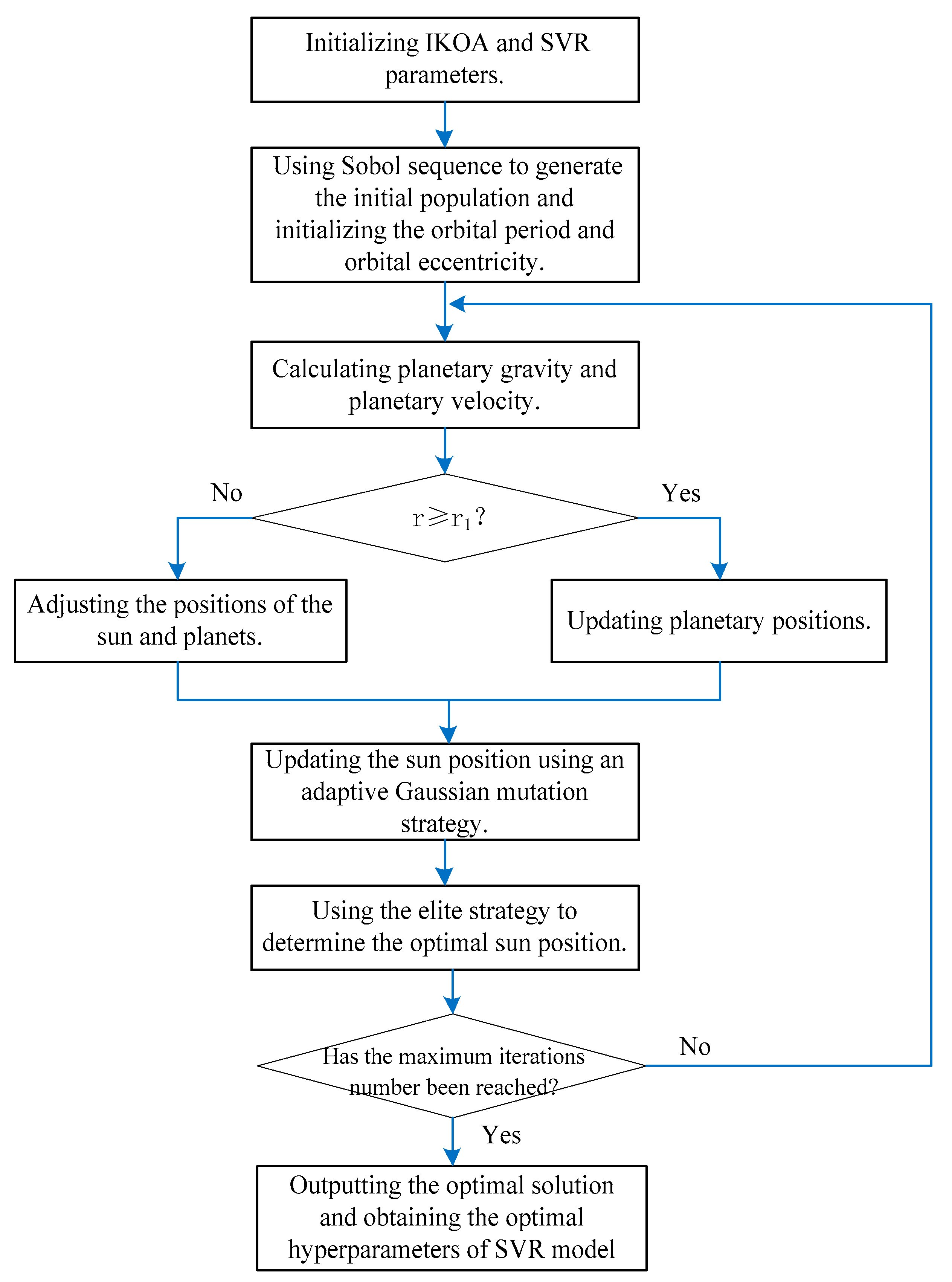
To address the drawback of KOA being prone to falling into local optima, this paper proposed the IKOA method, which combined Sobol sequence generation and an adaptive Gaussian mutation strategy, to achieve intelligent optimization of key parameters in SVR models. The IKOA process was shown in Figure 5.

The specific steps of the IKOA method were as follows:

(1)

Initialized IKOA parameters, including initial population size $N$, population dimension dim, maximum iteration number $T_{\max }$, cycle control parameter $Tc$, initial gravitational parameter ${\mu }_0$, and gravitational decay factor ${\lambda }_1$. Initialized SVR parameters, including C and γ.

(2)

Used the Sobol sequence to generate the initial population and initialized the orbital period and orbital eccentricity.

The Sobol sequence was used to generate candidate solutions (planets) within the specified ranges of C and γ. Each planet contains a set of hyperparameters C and γ, forming the initial population. Calculating the fitness of each planet and selecting the planet with the minimum fitness as the Sun, the initial position of the population can be written as

$$X_i^j=X_{i,low}^j+K_i\cdot (X_{i,up}^j-X_{i,low}^j),$$

(1)

where $X_i^j$ is the position of the i-th planet in the j-th dimension; $K_i$ is the random number generated by the Sobol sequence for the i-th planet, $K_i\in \left[\begin{array}{c}0,1\end{array}\right]$; and $X_{i,up}^j$ and $X_{i,low}^j$ are the upper and lower bounds of the j-th dimension of the i-th planet, respectively.

The equations for initializing the orbital period and orbital eccentricity are as follows:

$$T_i=\left|r\right|,i=1,\dots ,N;$$

(2)

$$e_i=ran{d}_{\left[0,1\right]},i=1,\dots ,N,$$

(3)

where $r$ is a random number generated based on a normal distribution.

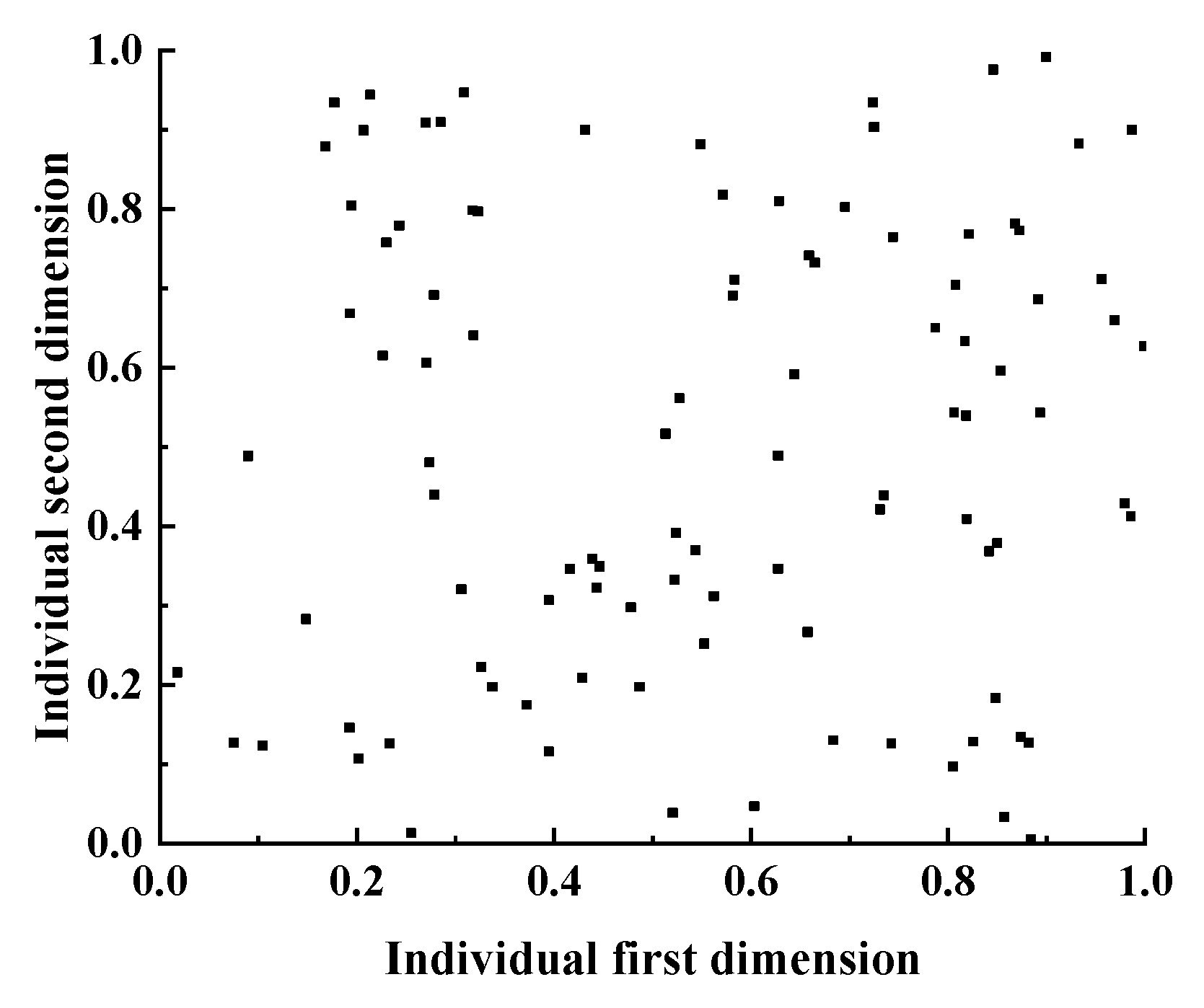
Traditional KOA uses a random number generation method for the initial population positions, which introduces uncertainty in the initial positions and may fall into local optima [20,21]. In contrast, by using the Sobol sequence to generate initial solutions, the generated random numbers can be evenly distributed in the solution space. To facilitate efficient optimization by the IKOA, we linearly normalized the search ranges of the SVM hyperparameters C and γ to the interval [0, 1]. The algorithm operates within a unified two-dimensional search space [0, 1]. The population size is set to 100, the dimension is 2, and the upper and lower bounds of the population position are 1 and 0, respectively. The initial population distributions generated by the random number method and the Sobol sequence method within the normalized space are shown in Figure 6 and Figure 7, respectively (Note: Figure 6 and Figure 7 are for visualization purposes only and use a sample size of 100 individuals; the actual experiment employed 30 individuals). For each fitness evaluation, the dimensional values of an individual are mapped back to their actual hyperparameter values. As shown in the figures, there is a significant difference in the scatter distribution characteristics between the two methods. The scatter points generated by random number generation are typically more densely distributed in certain regions and relatively sparse in others, with obvious blank areas. In contrast, the scatter points generated by the Sobol sequence generation are more uniformly distributed across the entire space, ensuring a more comprehensive coverage of the entire search space and avoiding large areas of sample overlap or omission, thereby enhancing the global exploration ability of the algorithm in the initial stage and laying a better foundation for finding high-quality solutions.

(3)

Calculating planetary gravity and planetary velocity.

The expressions of planetary gravity are

$$F_{g_i}\left(t\right)=e_i\cdot \mu \left(t\right)\cdot {\displaystyle \frac{{\overline{M}}_s\cdot {\overline{m}}_i}{{\overline{R}}_i^2\left(t\right)+\epsilon }}+r_1;$$

(4)

$$R_i(t)=\sqrt{{\displaystyle \sum _{j=1}^{\dim }{(X_{Sj}(t)-X_{ij}(t))}^2}};$$

(5)

$$\mu \left(t\right)={\mu }_0\times \exp (-{\lambda }_1{\displaystyle \frac{t}{T_{\max }}}),$$

(6)

where $F_{g_i}\left(t\right)$ is the planetary gravity of the i-th planet at the t-th iteration; $F_g$ is the planetary gravity; $e_i$ is the orbital eccentricity of the i-th planet; $\mu \left(t\right)$ is the gravitational parameter, which is an exponentially decreasing function of the number of iterations t, used to control search accuracy; ${\overline{M}}_s,{\overline{m}}_i$ are the normalized values of the solar mass and planetary mass, respectively; ${\overline{R}}_i^2\left(t\right)$ is the squared normalized Euclidean distance between the Sun and the planet at the t-th iteration; $r_1$ is a randomly generated number between 0 and 1; $\epsilon$ is a small value to prevent the denominator from becoming zero; $X_s(t),X_i(t)$ are the positions of the Sun and the i-th planet at the t-th iteration, respectively; $X_{Sj}(t)$ is the position of the Sun in the j-th dimension at the t-th iteration; and $X_{ij}(t)$ is the position of the i-th planet in the j-th dimension at the t-th iteration.

The equations of solar mass, planetary mass, and fitness are as follows:

$$M_s=r_2\times {\displaystyle \frac{fi{t}_s(t)-worst(t)}{{\displaystyle \sum _{k=1}^N\left(fi{t}_k(t)-worst(t)\right)}}};$$

(7)

$$M_s=r_2\times {\displaystyle \frac{fi{t}_s(t)-worst(t)}{{\displaystyle \sum _{k=1}^N\left(fi{t}_k(t)-worst(t)\right)}}};$$

(8)

$$fi{t}_s\left(t\right)=best\left(t\right)={\min }_{k\in 1,2,\dots ,N} {fit}_k(t);$$

(9)

$$worst\left(t\right)={\max }_{k\in 1,2,\dots ,N} {fit}_k(t),$$

(10)

where $M_s$ is the solar mass; $m_i$ is the planetary mass; $r_2$ is a randomly generated number between 0 and 1; $fi{t}_i(t)$ is the fitness of the i-th planet in the t-th iteration; $fi{t}_k(t)$ is the fitness of the k-th planet, $k\in 1,2,\dots ,N$, introduced to avoid conflicts with $fi{t}_i(t)$; $fi{t}_s\left(t\right)$ is the minimum value among the fitnesses of all planets in the t-th iteration; $best\left(t\right)$ is the minimum value among the fitnesses of all planets in the t-th iteration; $worst\left(t\right)$ is the maximum values among the fitnesses of all planets in the t-th iteration.

Planetary velocity represents the step size and direction of planetary movement in the search space. $\stackrel{-----}{R_i(t)}$ represents the normalized distance between the Sun and the planet; when $\overline{R_i(t)}\le 0.5$, the local exploitation formula is adopted to calculate planetary velocity; and when $\overline{R_i(t)}>0.5$, the global exploration formula is used. The expression is as follows:

$$V_i(t)=\left\{\begin{array}{l}\mathcal{l}\cdot \left(2r_4{X}_i-X_b\right)+\ddot{\mathcal{l}}\cdot \left(X_a-X_b\right)+\left(1-\overline{R_i\left(t\right)}\right)\cdot \mathcal{F}\cdot U_1\cdot r_5\cdot \left(X_{i,up}-X_{i,low}\right),\overline{R_i(t)}\le 0.5\hfill \\ r_4\cdot \mathcal{L}\cdot \left(X_a-X_i\right)+\left(1-\overline{R_i\left(t\right)}\right)\cdot \mathcal{F}\cdot U_2\cdot r_5\cdot \left(r_3{X}_{i,up}-X_{i,low}\right),\overline{R_i(t)}>0.5\hfill \end{array}\right.,$$

(11)

where $V_i\left(t\right)$ is the planetary velocity of the i-th planet at the t-th iteration; $X_a,X_b$ are the positions of two randomly selected planets; $X_{i,up},X_{i,low}$ are the maximum and minimum values of the planet positions at the t-th iteration; $R_i(t)$ is the Euclidean distance between the Sun and the i-th planet at the t-th iteration; $r_3,r_4,r_5$ are randomly generated numbers between 0 and 1; $U_1$ and $U_2$ are variables that can be either 0 or 1; when $r_5\le r_4$, $U_1$ takes 0, and otherwise it takes 1; when $r_3\le r_4$, $U_2$ takes 0, and otherwise it takes 1; $\mathcal{F}$ is a variable that can be either 1 or −1; and when $r_4\le 0.5$, $\mathcal{F}$ takes 1, and otherwise takes −1. Some variables in Equation (11) can be written as

$$\mathcal{l}=U\cdot (r_3\cdot (1-r_4)+r_4)\cdot {\left[\mu \left(t\right)\cdot \left(M_S+m_i\right)\left|{\displaystyle \frac{2}{R_i(t)+\epsilon }}-{\displaystyle \frac{1}{a_{i(t)}+\epsilon }}\right|\right]}^{{\displaystyle \frac{1}{2}}};$$

(12)

$$\ddot{\mathcal{l}}=\left(\begin{array}{c}1-U\end{array}\right)\cdot \left(\begin{array}{c}{r}_3\cdot \left(\begin{array}{c}1-r_5\end{array}\right)+r_5\end{array}\right)\cdot {\left[\mu \left(t\right)\cdot \left(M_S+m_i\right)\left|{\displaystyle \frac{2}{R_i(t)+\epsilon }}-{\displaystyle \frac{1}{a_{i(t)}+\epsilon }}\right|\right]}^{{\displaystyle \frac{1}{2}}};$$

(13)

$$\mathcal{L}={\left[\mu \left(t\right)\cdot \left(M_S+m_i\right)\left|{\displaystyle \frac{2}{R_i(t)+\epsilon }}-{\displaystyle \frac{1}{a_{i(t)}+\epsilon }}\right|\right]}^{{\displaystyle \frac{1}{2}}};$$

(14)

$$a_{i(t)}=r_3\times {\left[T_i^2\times {\displaystyle \frac{\mu (t)\times (M_s+m_i)}{4{\pi }^2}}\right]}^{{\displaystyle \frac{1}{3}}},$$

(15)

where $a_{i(t)}$ is the semi-major axis of the elliptical orbit of the i-th planet, controlling the amplitude of the planet’s motion; the larger $a_{i(t)}$ is, the broader the search range is; $U$ is a variable that takes 0 or 1; when $r_5\le r_6$, $U$ takes 0, and otherwise takes 1; $r_6$ is a randomly generated number between 0 and 1; and $\epsilon$ is a small value to prevent the denominator from becoming zero.

When $r\ge r_1$, proceed to step (4) to update the planetary positions, and when $r<r_1$, proceed to step (5) to adjust the positions of the Sun and planets.

(4)

Updating planetary positions. During the simulation of planetary motion around the Sun, periodically switch the search direction to break through local optimal regions, providing planets with better opportunities to explore the entire space [23]. When $r\ge r_1$, the new planetary position is updated as follows:

$$X_i\left(t+1\right)=X_i\left(t\right)+\mathcal{F}\cdot V_i\left(t\right)+\left(F_{g_i}\left(t\right)+\left|r\right|\right)\cdot U\cdot \left(X_S\left(t\right)-X_i\left(t\right)\right),$$

(16)

where $X_i\left(t+1\right)$ is the position of the i-th planet at the t + 1 iteration; $r$ is a randomly generated number between 0 and 1.

(5)

Adjusting the positions of the Sun and planets. When $r<r_1$, update the planetary positions and simulate the changes in the distance between the Sun and planets with the number of iterations. When planets are close to the Sun, the development operator is activated to enhance convergence speed, and KOA focuses on optimizing development; when planets are far from the Sun, they adjust their distances from the Sun, and KOA focuses on optimizing the exploration operation [24]. The mathematical model expression is as follows:

$$X_i\left(t+1\right)=X_i\left(t\right)\cdot U_1+\left(1-U_1\right)\cdot \left({\displaystyle \frac{X_i\left(t\right)+X_S+X_a\left(t\right)}{3.0}}+h\cdot \left({\displaystyle \frac{X_i\left(t\right)+X_S+X_a\left(t\right)}{3.0}}-X_b\left(t\right)\right)\right),$$

(17)

where $h$ is the adaptive factor used to control the distance between the Sun and the planet in the t-th iteration, expressed as

$$h={\displaystyle \frac{1}{e^{\eta r}}},$$

(18)

where $\eta$ is a linear decreasing factor from 1 to −2, expressed as

$$\eta =(a_2-1)\times r_4+1,$$

(19)

and where $a_2$ is the loop control parameter that gradually decreases from −1 to −2 over $T_{\max }$ loops during the entire optimization process, expressed as

$$a_2=-1-\left({\displaystyle \frac{t\%\frac{T_{max}}{T_c}}{\frac{T_{max}}{T_c}}}\right).$$

(20)

(6)

Updating the Sun’s position using an adaptive Gaussian mutation strategy.

KOA may encounter situations where the Sun’s position remains unchanged after multiple iterations, and the Sun’s position cannot escape the local optimum after the perturbation weakens in the later stages of exploration. This premature convergence problem is particularly prominent in multi-peak optimization problems, leading to the final optimization result deviating from the global optimum solution [25]. To address this issue, this paper introduces an adaptive Gaussian mutation strategy into the algorithm’s iteration process. By dynamically adjusting the intensity and frequency of Gaussian mutations during algorithm execution, individuals can escape from local optima and regain search activity when trapped in a local optimum. Compared to fixed-parameter mutation methods, the adaptive mechanism uses the current individual’s position as an adaptive adjustment factor to dynamically adjust the perturbation intensity of Gaussian mutation and flexibly regulate the mutation range. This approach maintains local search precision while enhancing global exploration capabilities. The adaptive Gaussian mutation strategy is expressed as

$$X_s^{\prime }=\left\{\begin{array}{lll}{X}_s\times (1+\mathcal{N}(0,\sigma )),\hfill & b_1<b_2\hfill & \hfill \\ X_s,\hfill & b_1\ge b_2\hfill & \hfill \end{array}\right.,$$

(21)

where ${X_s}^{\prime }$ is the Sun’s position after mutation; $X_s$ is the Sun’s position before mutation; $b_1$ and $b_2$ are randomly generated numbers between 0 and 1; $\mathcal{N}(0,\sigma )$ is a normal random variable with a mean of 0 and a standard deviation of $\sigma$; $\sigma$ is the standard deviation of normal mutation, which controls the mutation intensity, and its expression is as follows:

$$\sigma =e^{-2\cdot {\displaystyle \frac{t}{T_{\max }}}}.$$

(22)

From the above equation, the standard deviation curve with the number of iterations can be obtained, as shown in Figure 8.

(7)

Using the elite strategy to determine the optimal Sun position

The elite strategy is used to determine the optimal Sun position, expressed as

$$X_{s,new}(t+1)=\left\{\begin{array}{ll}{X}_s(t+1),X_s(t+1)\le X_s(t)\hfill & \hfill \\ X_s(t),X_s(t+1)>X_s(t)\hfill & \hfill \end{array}\right.,$$

(23)

where $X_{s,new}(t+1)$ represents the retained position of the Sun.

(8)

Determining whether the maximum number of iterations has been reached. If so, the iteration ends, and the results C and γ are output. If not, return to step (3).

4.2. Building the SVR Model

SVR is a machine learning algorithm based on the principle of minimizing structural risk. Its fundamental objective is not merely to fit the training data, but to minimize the model’s generalization error by seeking a regression function f(x) that is as “smooth” as possible while maintaining predictive accuracy.

The implementation of SVR relies on the configuration of three core hyperparameters: C, γ, and the insensitivity loss parameter ε. These three parameters collectively determine the model’s performance: C: balances the model’s structural risk against empirical risk. A larger C value forces the model to reduce training error, but this may come at the cost of sacrificing the model’s generalization ability, leading to overfitting. Conversely, a smaller C value places greater emphasis on reducing model complexity, potentially resulting in the model underfitting the training data. γ: When using a radial basis function (RBF) kernel, γ determines the spatial influence range of individual training samples. A high γ value indicates a small influence range, where only nearby data points affect predictions, potentially causing the model to focus excessively on local details and overfit. A low γ value indicates a large influence range, resulting in a smoother model but potentially failing to capture complex data variations, leading to underfitting. ε: Defines the width of the ε-insensitivity band. Loss is only computed when the prediction error of a sample point exceeds this range. Thus, ε controls the model’s precision and tolerance for error. A larger ε increases the model’s tolerance for error, resulting in a simpler model; a smaller ε makes the model more sensitive to error, leading to a more complex model.

Mathematically, for the training set ${\left(x_i,y_i\right)}_{i=1}^n$, SVR performs regression by constructing a separating hyperplane or an approximating function in the high-dimensional feature space:

$$f(x)=w^T\varphi (x)+b,$$

(24)

where $f(x)$ is the objective function; $\varphi (x)$ is a mapping function; $w^T$ is the weight vector; and $b$ is the bias term.

By introducing slack variables ${\xi }_i,{\xi }_i^{*}$, the optimal f(x) can be found by solving the following convex quadratic programming problem:

$$\underset{w,b}{\min }{\displaystyle \frac{1}{2}}{‖w‖}^2+C{\displaystyle \sum _{i=1}^n\left({\xi }_i+{\xi }_i^{*}\right)}.$$

(25)

The constraints are as follows:

$$\left\{\begin{array}{l}{y}_i-f\left(x_i\right)\le \epsilon +{\xi }_i\hfill \\ f\left(x_i\right)-y_i\le \epsilon +{\xi }_i^{*}\hfill \\ {\xi }_i,{\xi }_i^{*}\ge 0\hfill \end{array}\right..$$

(26)

By introducing the Lagrange multiplier ${\alpha }_i,{\alpha }_i^{\prime }$ and taking the partial derivative with respect to the parameter, the minimization problem can be transformed into the following dual problem:

$$\begin{array}{l}minR({\alpha }^{\prime },\alpha )={\displaystyle \frac{1}{2}}{\displaystyle \sum _{i=1j=1}^n({\alpha }_i^{\prime }-{\alpha }_i)({\alpha }_j^{\prime }-{\alpha }_j)K(x_i,x_j)}+\\ \epsilon {\displaystyle \sum _{i=1}^n({\alpha }_i^{\prime }+{\alpha }_i)}-{\displaystyle \sum _{i=1}^n{y}_i}({\alpha }_i^{\prime }-{\alpha }_i)\end{array},$$

(27)

where $K\left(x_i,x\right)$ is the kernel function.

The final SVR decision function is

$$f(x)={\displaystyle \sum _{i=1}^n\left({\alpha }_i-{\alpha }_i^{*}\right)K\left(x_i,x\right)+b}.$$

(28)

4.3. IKOA-SVR Model Training

Based on the intelligent identification training dataset, a Gaussian radial basis kernel function is used as the kernel function for the SVR model. A multi-step sliding cross-validation method is proposed to train the SVR model, which involves randomly and uniformly dividing the training set into n subsets. The training set is randomly and uniformly divided into n subsets, and two subsets are selected as the internal testing dataset in sequence (without repetition), while the remaining subsets are used as the internal training dataset. There will be C(n,2) situations. Each situation is trained using the internal training dataset and tested using the internal testing dataset, with the cross-validation process repeated C(n,2) times to ensure that each pair of subsets is used as the internal testing dataset exactly once.

Compared to traditional K-fold cross-validation, which uses only a single data subset as the testing set in each iteration, the multi-step sliding cross-validation method selects two data subsets to form the testing set. One primary source of uncertainty in traditional K-fold cross-validation is the variance within the testing set during a single iteration. Multi-step sliding cross-validation increases the number of testing samples by using two subsets as the testing set in each iteration, effectively smoothing out randomness in single-run evaluations and thereby reducing the variance in performance assessments. Finally, averaging the results from C(n,2) exhaustive tests further ensures the high stability of the final evaluation outcomes.

Traditional K-fold cross-validation only tests a model’s ability to learn from n − 1 subsets and generalize to a single unknown subset. In contrast, multi-step sliding cross-validation comprehensively evaluates a model’s capacity to learn from n − 2 subsets and generalize to any combination of two unknown subsets. This approach enables the model to not only adapt to variations within a single data distribution but also overcome challenges posed by different combinations of data distributions, thereby enhancing its generalization capability against data heterogeneity.

The C(n,2) iterations far exceed the n iterations of traditional K-fold cross-validation. This approach systematically eliminates random biases arising from specific data partitioning schemes, ensuring evaluation outcomes are not dependent on any single random split. Consequently, the model assessment achieves greater comprehensiveness and thoroughness.

For each test, an intelligent identification model for valve internal leakage is constructed using Mean Squared Error (MSE) as the fitness function. The specific formula is as follows:

$$\mathrm{MSE}={\displaystyle \frac{1}{m}}{\displaystyle \sum _{i=1}^m{\left(y_i-{\widehat{y}}_i\right)}^2},$$

(29)

where $m$ is the number of samples in the training dataset; $y_i$ is the actual value of the i-th sample in the training dataset; and ${\widehat{y}}_i$ is the predicted value of the i-th sample in the training dataset.

To objectively and quantitatively evaluate the model performance proposed in this paper, in addition to MSE, four performance metrics are used to evaluate the model performance, including Root Mean Squared Error (RMSE), Mean Absolute Error (MAE), Mean Absolute Percentage Error (MAPE), and determination coefficient (R²). The final performance evaluation result of the model is obtained by taking the average of the performance results from C(n,2) tests. By using five performance metrics to evaluate the identification results, the identification accuracy and reliability of the model can be comprehensively measured from different perspectives.

The equations for these performance metrics are as follows:

$$\mathrm{RMSE}=\sqrt{{\displaystyle \frac{1}{m}}{\displaystyle \sum _{i=1}^m{\left(y_i-{\widehat{y}}_i\right)}^2}};$$

(30)

$$\mathrm{MAE}={\displaystyle \frac{1}{m}}{\displaystyle \sum _{i=1}^m|}{y}_i-{\widehat{y}}_i|;$$

(31)

$$\mathrm{MAPE}={\displaystyle \frac{100\%}{m}}{\displaystyle \sum _{i=1}^m\left|\frac{{\widehat{y}}_i-y_i}{y_i}\right|};$$

(32)

$$R^2=1-{\displaystyle \frac{{\displaystyle \sum _{i=1}^N{({\overline{y}}_i-{\widehat{y}}_i)}^2}}{{\displaystyle \sum _{i=1}^N{(y_i-{\overline{y}}_i)}^2}}}.$$

(33)

MSE, RMSE, and MAE are used to measure the deviation degree between the identification value and the actual value. The smaller the value, the smaller the identification error and the higher the accuracy. MAPE represents the identification error as a percentage of the actual value, which can more intuitively reflect the relative error size of the identification result. The R² reflects the fitness degree of the model, and the closer the R² is to 1, the closer the identification result is to the actual value.

5. Case Studies

The study focuses on the main steam drain pipe valves of a 600 MW thermal power station. The rated temperature of the main steam is 600 °C, and the rated pressure is 24.2 MPa. The structure diagram of the main steam drain pipe valve is shown in Figure 1. The calculation conditions are as follows: drain pipe length is 8.0 m, drain pipe diameter is 0.09 m, drain pipe wall thickness is 0.008 m, and drain pipe insulation layer thickness is 0.11 m.

The dataset is constructed with the inlet steam temperature $T_{In}$ and inlet steam pressure $P_{In}$, with pipe wall temperature $T_B$ as input parameters and the valve internal leakage quantification $G_L$ as output parameters. Due to the complex operating conditions and wide range of parameter variations in the unit, it is difficult to establish a dataset covering various operating conditions based on the actual operating data of the unit. Therefore, this paper simulates and generates a dataset based on the calculation model for valve internal leakage established in Section 2 [28].

The model in this paper is developed based on the PyCharm 2024.1.1 integrated environment and implemented using the Python 3.8 programming language. The computer configuration for model training is 13th Gen Intel (R) Core (TM) i5-13500H (2.60 GHz) CPU and NVIDIA GeForce RTX 4050 Laptop 6 GB GPU.

To evaluate the identification performance of the proposed IKOA-SVR method, two types of test cases are designed based on different testing datasets. The first is the In-Distribution (ID) test, where the testing dataset shares the same distribution as the training data, used to validate the model’s performance on data similar to the training data. The other is the Out-Of-Distribution (OOD) test, where the testing dataset differs from the training data distribution. This evaluates the model’s generalization capability, robustness, and resilience to unknown scenarios, which is crucial for assessing its practicality in real industrial settings. For the OOD test dataset sources, this paper further analyzes two scenarios: noise injection and Region-Holdout.

5.1. In-Distribution (ID) Test

Based on the main steam rated parameters, the parameter ranges and variation increments for generating the simulation dataset are shown in

Table 1. Parameter Range for Simulated Dataset Generation.

No.	Parameter Name	Start Value	End Value	Step Length
1	Main Steam Temperature/°C	570	610	5
2	Main Steam Pressure/MPa	10	26	2
3	Valve Internal Leakage/kg/h	20	200	2

.

Based on Table 1, a total of 5760 simulated datasets are obtained. After normalizing the data, the dataset is randomly divided into a training dataset and a testing dataset, with the training dataset accounting for 80% and the testing dataset accounting for 20%, forming the final intelligent identification training dataset and testing dataset.

The initial parameters of IKOA are set as follows: initial population size N is 30; population dimension dim is 2; maximum number of iterations $T_{\max }$ is 10; cycle control parameter $Tc$ is 3; initial gravitational parameter ${\mu }_0$ is 0.1; and gravitational decay factor ${\lambda }_1$ is 15. The initial parameters of SVR are set as follows: the range of C is [0.1, 1000], and the range of γ is [0.01, 1].

The IKOA method is used for self-optimization of SVR key parameters. During the optimization process, the values of parameters C and γ are continuously adjusted. The MSE on the testing dataset is used as the fitness function to find the optimal hyperparameter combination, as shown in Figure 9.

It can be observed that there are many extrema points in the optimization process. The algorithm must effectively avoid falling into local optima and achieve global optimization when solving the fitness function. During the optimization process, IKOA can repeatedly escape local optima and continue to search for better solutions, demonstrating excellent ability to escape local optimum traps. The optimal hyperparameters C and γ obtained through IKOA are 354.83 and 0.589. The optimization results indicate that IKOA effectively enhances the global search capability of the traditional KOA while maintaining stability and significantly improving the convergence performance.

To verify the superiority of parameter identification of IKOA, a comparative analysis was conducted on six algorithms: IKOA, KOA, PSO, Random Search (RS), Grid Search (GS), and Bayesian Optimization (BO). Figure 10 shows the MSE curves of four algorithms during the training process as a function of the number of iterations. According to Figure 10, IKOA tends to stabilize after four iterations, with the MSE approaching 0.59, which is the smallest value; after six iterations, KOA tends to stabilize with the MSE approaching 2.75, which is greater than IKOA; after five iterations, BO tends to stabilize with the MSE approaching 3.32, ranking third; and after six iterations, PSO tends to stabilize with the MSE approaching 5.81, which is higher than others. It can be seen that IKOA has the fastest convergence speed, the smallest identification error, and the highest identification accuracy compared to KOA, PSO, and BO.

IKOA-SVR, KOA-SVR, PSO-SVR, RS-SVR, GS-SVR, and BO-SVR methods were used for intelligent identification of valve internal leakage on the training and testing datasets, respectively.

Table 2. Analysis results of five performance metrics of six methods.

Method	Training Dataset						Testing Dataset
	MSE	RMSE	R2	MAE	MAPE	Operating Time (s)	MSE	RMSE	R2	MAE	MAPE
IKOA-SVR	0.59	0.77	0.9998	0.45	0.0038	2794	0.65	0.81	0.9998	0.49	0.0043
KOA-SVR	2.75	1.66	0.9990	1.05	0.0093	733	3.08	1.75	0.9988	1.12	0.0096
PSO-SVR	5.81	2.41	0.9978	1.57	0.0140	623	6.30	2.51	0.9977	1.65	0.0144
RS-SVR	8.07	2.84	0.9970	1.86	0.0169	50	9.46	3.08	0.9963	2.22	0.0230
GS-SVR	3.91	1.98	0.9985	1.14	0.0097	173	4.46	2.11	0.9973	1.23	0.0108
BO-SVR	3.32	1.82	0.9987	1.15	0.0101	762	3.63	1.77	0.9984	1.16	0.0104

shows the analysis results of five performance metrics in the training and testing datasets.

Table 2 shows that for the testing dataset, IKOA-SVR achieves the lowest prediction error in terms of forecasting accuracy. Its MSE is only 0.65, representing a significant reduction of approximately 79% compared to the next best model: KOA-SVR (3.08). Simultaneously, it demonstrates the best performance across all metrics, including RMSE (0.81), MAE (0.49), and MAPE (0.0043). In terms of goodness of fit, IKOA-SVR also demonstrated superior performance. Its R² reaches 0.9998, approaching 1, indicating that the model constructed by this algorithm explains the vast majority of variance in the target variable and can be effectively applied to new, unseen data.

Figure 11 compares the six methods on five performance metrics in the testing dataset. According to Table 2 and Figure 11, for the testing dataset, the analysis results of the five performance metrics of the six methods are similar to those of the training dataset. In terms of the difference in MSE between the training and testing datasets, it can be found that the IKOA-SVR method has the smallest difference, with a value of 0.06, indicating that no overfitting has occurred. At the same time, it should be noted that for the training dataset, the IKOA-SVR method takes 2794 s, with the longest training duration. The reason is that IKOA-SVR uses a multi-step sliding cross-validation method to train the model and searches more meticulously during the iterative optimization process.

In order to better observe the identification results, 30 samples from the testing dataset are selected for analysis. Figure 12 shows the intelligent identification results of valve internal leakage, and Figure 13 shows the scatter plot of the identification results. As shown in the figures, the identification results curve of IKOA-SVR is closest to the actual value curve, and the scatter points are also closely around the consistency line, followed by KOA-SVR, and the worst is RS-SVR. This indicates that IKOA-SVR has the highest identification accuracy, followed by KOA-SVR, and RS-SVR is the worst.

The main improvements of the IKOA in this paper are two-fold: Sobol sequence generation and adaptive Gaussian mutation strategy. To further evaluate the effectiveness of each improvement in the IKOA, an ablation study was conducted using the control variable method. The objective was to investigate the impact of individual improvements on KOA-SVR performance. The ablation study results based on the testing dataset are shown in

Table 3. Ablation study results.

	MSE	RMSE	R2	MAE	MAPE
Only Sobol sequence generation	2.18	1.48	0.9991	0.84	0.0082
Only adaptive Gaussian mutation strategy	0.88	0.94	0.9996	0.53	0.0052
IKOA-SVR	0.65	0.81	0.9998	0.49	0.0043
KOA-SVR	3.08	1.75	0.9988	1.12	0.0096

.

As shown in Table 3, the ablation study results demonstrate the effectiveness of the IKOA across various improvement measures. Taking the MSE metric as an example, the KOA exhibits the highest MSE value of 3.08. In contrast, the MSE for the “Only Sobol sequence generation” is 2.18, outperforming KOA. This indicates that using Sobol sequences to generate a uniform initial population enhances optimization performance. The MSE of the “Only adaptive Gaussian mutation strategy” is 0.88, outperforming the previous two and approaching the 0.65 achieved by IKOA. This indicates that the adaptive Gaussian mutation strategy contributes most significantly to improving optimization performance. The ablation study results for metrics such as RMSE, MAE, MAPE, and R² are similar to those of MSE.

Figure 14 shows the intelligent identification results of the ablation study. As shown in the figure, the identification results curve of IKOA-SVR is closest to the actual value curve, followed by the “Only adaptive Gaussian mutation strategy”, with KOA-SVR performing the worst. “Only Sobol sequence generation” slightly outperforms KOA-SVR. This demonstrates that compared to the standalone KOA-SVR, incorporating these improvements enhances all performance metrics, with the “Only adaptive Gaussian mutation strategy” yielding the most pronounced effect.

5.2. OOD Test Based on Noise Injection

By incrementally adding white noise to the testing dataset, we systematically simulate data distribution shifts ranging from minor to significant, enabling quantitative analysis of model performance degradation. The OOD test dataset construction method is as follows: Using the testing dataset from Section 5.1 as a baseline, Gaussian white noise is systematically added to each input parameter of this dataset to simulate potential data distribution shifts encountered in real-world applications, thereby constructing the OOD test dataset. To ensure noise intensity correlates with the original data scale, the amplitude of white noise is scaled relative to the standard deviation ${\sigma }_j$ of each input parameter in the testing dataset. The white noise level ${ϵ}_{i,j}$ is incremented $\alpha$ from 1% to 10% in 1% increments, with ${ϵ}_{i,j}$ following a Gaussian distribution. The noise-augmented testing dataset ${x^{\prime }}_{\mathrm{test}}$ can then be expressed as

$$x_{\mathrm{test},i,j}^{\prime }=x_{\mathrm{test},i,j}+{ϵ}_{i,j}$$

(34)

where $x_{\mathrm{test},i,j}$ represents the original testing dataset, and ${ϵ}_{i,j}$ denotes white noise, calculated as follows:

$${ϵ}_{i,j}~\mathcal{N}(0,{(\alpha /100\times {\sigma }_j)}^2)$$

(35)

Based on the testing dataset with added noise, the OOD test is conducted on IKOA-SVR. The test results for various metrics are shown in

Table 4. OOD test results for various metrics of IKOA-SVR.

White Noise Ratio	R2	MSE	RMSE	MAE	MAPE
0%	0.9998	0.65	0.81	0.49	0.0043
1%	0.9991	1.57	1.25	0.71	0.0062
2%	0.9974	2.37	1.54	1.16	0.0084
3%	0.9943	5.17	2.27	1.25	0.0117
4%	0.9891	7.17	2.68	1.62	0.0145
5%	0.9863	10.99	3.31	2.01	0.0180
6%	0.9782	15.17	3.90	2.52	0.0214
7%	0.9734	19.89	4.46	3.09	0.0251
8%	0.9671	25.91	5.09	3.65	0.0293
9%	0.9595	30.23	5.50	4.23	0.0340
10%	0.9508	36.99	6.08	4.84	0.0391

. Taking the scenarios with 1%, 5%, and 10% added noise as examples, the resulting identification curves are depicted in Figure 15.

As shown in Table 4, with increasing white noise, MSE, RMSE, MAE, and MAPE all increase to varying degrees, while R² continues to decrease. This indicates a decline in the robustness of IKOA-SVR. Similar observations can be made in Figure 15: as white noise increases, the identification curve deviates further from the actual values, indicating a deterioration in identification accuracy. Taking the R² metric as an example, at a 1% white noise level, the model’s R² remains as high as 0.9991. This indicates that under minor distribution shifts, the model’s performance degradation is negligible. Even when the noise proportion increases to 5%, the R² value remains robustly at 0.9863, while the MSE also remains relatively small. This demonstrates that IKOA-SVR exhibits strong robustness against mild to moderate data perturbations and possesses reliable performance and practical potential when handling noisy and fluctuating data commonly encountered in real industrial processes.

Using R² as the performance metric, the performance degradation curves of the six methods as white noise intensifies are shown in Figure 16. The figure reveals that all six methods exhibit identical performance trends with white noise variation: their performance curves decline as white noise intensifies, indicating continuous degradation. Comparatively, the performance curve of IKOA-SVR exhibits the gentlest decline, indicating minimal degradation, while GS-SVR shows the steepest decline, indicating the most significant degradation.

5.3. OOD Test Based on Region-Holdout

To rigorously evaluate the generalization capability and robustness of the developed model when confronted with specific input space regions not covered by the training data distribution, this paper additionally incorporates the OOD test based on Region-Holdout. When simulating the dataset, the original dataset is divided into three non-contiguous regions. The regions at both ends of the dataset are used as the training dataset, while the middle region serves as the testing dataset. This ensures the testing data distribution is clearly outside the training data distribution, thereby simulating novel operating conditions or unexplored parameter ranges that may be encountered in actual systems.

The parameter ranges and variation increments used when simulating the training dataset are shown in

Table 5. Parameter ranges for simulated training dataset generation.

Data Segment	Parameter Name	Start Value	End Value	Step Size
Data Segment1	Main Steam Temperature/°C	570	595	3
	Main Steam Pressure/MPa	10	23	1
	Valve Internal Leakage/kg/h	30	100	2
Data Segment2	Main Steam Temperature/°C	605	610	2
	Main Steam Pressure/MPa	25	27	0.5
	Valve Internal Leakage/kg/h	140	200	2

. The parameter ranges and variation increments used when simulating the testing dataset are shown in

Table 6. Parameter ranges for simulated testing dataset generation.

No.	Parameter Name	Start Value	End Value	Step Size
1	Main Steam Temperature/°C	595	605	2
2	Main Steam Pressure/MPa	23	25	0.4
3	Valve Internal Leakage/kg/h	100	140	2

.

The OOD test results for six methods are shown in

Table 7. OOD test results of six methods.

Method	R2	MSE	RMSE	MAE	MAPE
IKOA-SVR	0.9834	7.58	2.75	1.53	0.0137
KOA-SVR	0.9554	15.35	3.92	2.57	0.0228
PSO-SVR	0.9265	19.22	4.38	3.08	0.0263
RS-SVR	0.9656	11.31	3.36	2.01	0.0180
GS-SVR	0.9222	19.81	4.45	3.03	0.0264
BO-SVR	0.9589	14.88	3.86	2.58	0.0225

. A radar chart of OOD test performance for six methods is shown in Figure 17.

Combining Table 2 and Table 7 reveals that during the OOD test, the MSE, RMSE, MAE, and MAPE metrics of all six methods increased to varying degrees, while R² decreased. This indicates that when testing data lies outside the distribution of training data, the generalization capability and robustness of all six methods diminish. Relatively speaking, IKOA-SVR exhibits the smallest changes across all metrics, indicating its robustness is the best among the six methods. Taking the R² metric as an example, IKOA-SVR still maintains a high level of 0.9834. This demonstrates that the model retains good extrapolation capability in unknown regions beyond the training data boundaries. Despite the clear regional differences in data distribution between the testing dataset and the training dataset, IKOA-SVR still maintains high prediction accuracy and goodness-of-fit.

Figure 17 presents a normalized performance radar chart for six methods across five metrics. In this chart, the optimal performance for each metric is mapped to 1, while the worst performance is mapped to 0. Consequently, the area enclosed by the polygon directly reflects the overall quality of the model’s performance. The diagram reveals that IKOA-SVR (blue polygon) demonstrates absolute dominance in performance. Its polygon vertices achieve the maximum value of 1.0 across all five evaluation axes, proving that it simultaneously attains the highest prediction accuracy (maximum R²) while minimizing all types of prediction errors (MSE, RMSE, MAE, and MAPE). This highlights its exceptional and comprehensive optimization capabilities. The other five methods lag significantly behind, highlighting pronounced performance gaps. This strongly confirms that the superiority of IKOA-SVR is comprehensive and robust, rather than an isolated performance under specific evaluation metrics.

6. Conclusions

Valves are critical auxiliary equipment in thermal power stations. Accurately assessing valve internal leakage quantification is of great significance for ensuring the safe and economical operation of a thermal power station. This paper proposed an intelligent valve internal leakage identification method that integrated the IKOA method with SVR. Taking the main steam drain pipe valve as an example, the method was validated through simulation case studies. Using MSE, RMSE, MAE, MAPE, and R² as performance metrics, IKOA-SVR, KOA-SVR, PSO-SVR, RS-SVR, GS-SVR, and BO-SVR methods were used to compare and analyze the training and testing datasets, respectively. The main conclusions of the paper are as follows:

(1)

The proposed IKOA method, which introduced Sobol sequence generation and adaptive Gaussian mutation strategy, can effectively solve the problems of local optima and overfitting commonly encountered in the KOA optimization process, thus possessing stronger global search capability.

(2)

By optimizing SVR key parameters using the IKOA method and training the IKOA-SVR model with a multi-step sliding cross-validation method, the difficulty in selecting key parameters of the SVR model can be effectively addressed, thereby improving identification accuracy. However, while improving search accuracy, it also increases the running time, resulting in the slowest model training speed.

(3)

Whether it is the training dataset or the testing dataset, compared to the other five methods, the IKOA-SVR method has the smallest MSE, RMSE, MAE, and MAPE values for identification results, and the largest R² value, indicating that the IKOA-SVR method has the strongest generalization ability, the best effect in improving fitting ability, the smallest identification error, the highest identification accuracy, and is closer to the actual value.

(4)

During the OOD test based on noise injection, the performance curves of all six methods decay as the white noise intensity increases in the testing dataset. By comparison, IKOA-SVR exhibits the least performance degradation and maintains strong robustness when confronted with mild to moderate data perturbations. During the OOD test based on Region-Holdout, both the generalization capability and robustness of all six methods decreased. In comparison, IKOA-SVR exhibits the smallest changes across all metrics, demonstrating the most optimal robustness.

This paper proposed the IKOA-SVR method for intelligent identification of valve internal leakage in a thermal power station, but there are still the following issues that need to be further improved in future research.

(1)

The constructed dataset is simulated based on the calculation model of valve internal leakage established in Section 2, rather than actual operating data from the unit, and its reliability needs further verification.

(2)

Many intelligent identification methods, such as GA, SOA, WOA, etc., have the potential to solve this problem. The paper only compared IKOA-SVR, KOA-SVR, PSO-SVR, RS-SVR, GS-SVR, and BO-SVR, which is not comprehensive enough. In the future, comparative analysis should be conducted with more intelligent identification methods.

(3)

The IKOA-SVR method has a slow training speed and a long testing running time. To increase its practicality, the method should be further optimized while ensuring identification accuracy to reduce running time.