Solving Nonlinear Energy Supply and Demand System Using Physics-Informed Neural Networks

Abstract

Nonlinear differential equations and systems play a crucial role in modeling systems where time-dependent factors exhibit nonlinear characteristics. Due to their nonlinear nature, solving such systems often presents significant difficulties and challenges. In this study, we propose a method utilizing Physics-Informed Neural Networks (PINNs) to solve the nonlinear energy supply–demand (ESD) system. We design a neural network with four outputs, where each output approximates a function that corresponds to one of the unknown functions in the nonlinear system of differential equations describing the four-dimensional ESD problem. The neural network model is then trained, and the parameters are identified and optimized to achieve a more accurate solution. The solutions obtained from the neural network for this problem are equivalent when we compare and evaluate them against the Runge–Kutta numerical method of order 5(4) (RK45). However, the method utilizing neural networks is considered a modern and promising approach, as it effectively exploits the superior computational power of advanced computer systems, especially in solving complex problems. Another advantage is that the neural network model, after being trained, can solve the nonlinear system of differential equations across a continuous domain. In other words, neural networks are not only trained to approximate the solution functions for the nonlinear ESD system but can also represent the complex dynamic relationships between the system’s components. However, this approach requires significant time and computational power due to the need for model training. Furthermore, as this method is evaluated based on experimental results, ensuring the stability and convergence speed of the model poses a significant challenge. The key factors influencing this include the manner in which the neural network architecture is designed, such as the selection of hyperparameters and appropriate optimization functions. This is a critical and highly complex task, requiring experimentation and fine-tuning, which demand substantial expertise and time.

1. Introduction

Differential equations and their systems are powerful mathematical methods used to model problems across various real-world fields such as physics, engineering, economics, healthcare, energy, and others [1,2,3]. In the energy sector, the development of mathematical models for managing efficient energy supply and demand plays a crucial role in the flexible energy community with energy storage systems and renewable energy generation [4,5]. One notable application of differential equation systems is modeling the ESD system, which describes the dynamic relationship between energy supply, demand, and the distribution of energy across different regions based on development indicators of each area. The behavior of these variables is modeled through a system of differential equations, as formulated by Mei Sun et al. [6,7]. Research has shown that the ESD system exhibits chaotic properties [8], and the solutions to these differential equations are characterized by strong nonlinearity, making it highly complex to find an exact analytical solution. In practice, solving such systems of differential equations relies on approximate methods. The traditional mathematical approach in this case involves numerical methods. Most of these methods require discretizing the time and space domains into grids [9,10], so the solutions provided by numerical methods are often discrete sets of values. Additionally, numerical methods can face difficulties when solving complex nonlinear systems of equations.

Recently, with the explosive and increasingly powerful development of artificial intelligence, machine learning, and particularly deep learning methods, these techniques are being applied across numerous fields of science and engineering. One of the recent promising studies involves using deep neural networks to solve differential equations and their systems. The mathematical foundation of this method is based on the research of Cybenko [11], followed by the work of Hornik et al. [12], on the capability of neural networks to approximate continuous functions. Isaac et al. [13] introduced a novel approach, utilizing neural networks to solve both ordinary differential equations (ODEs) with initial and boundary conditions and partial differential equations (PDEs). Since then, many related studies have employed neural networks and developed them into the PINNs method [14,15] to solve complex problems such as [16,17,18,19,20,21]: the Navier–Stokes equations, Burgers’ equation, Schrödinger equation, Poisson equation, diffusion equation, Lorenz equation, and Volterra equations. Apart from dynamic models based on differential and differential-algebraic equations, many inverse problems can be formulated in terms of integral equations [22]. Research on applying neural networks to solve integro-differential equations has also been conducted [23,24].

The advantage of this method over traditional numerical approaches is its ability to solve complex problems, especially systems of strongly nonlinear equations, without the need to discretize the time and space domains [25,26]. Initially, the neural network only needs to be trained to solve the system of equations at a set of specific time points in the computational domain. Once the model is built, it can provide solutions for any point within the trained time domain; that means the solution of the neural network method is a continuous domain [14,27,28]. In other words, the neural network can be trained to approximate the solution function of the system of differential equations. Moreover, the flexibility of PINNs allows for training a model that integrates constraints from the system of differential equations with real-world data [25,26,27,28], which is particularly useful for modeling real-world applications such as the energy supply–demand problem. This helps to predict the supply–demand variables of the system in a way that is closer to reality.

In addition to its strengths, this method also has several limitations that require further investigation and improvement. Among these, computational efficiency is a critical factor to consider, as maintaining accuracy often demands a large amount of training data. This makes the training process for PINNs highly resource-intensive, especially when a large number of solutions are required or when the computational domain is complex, such as in nonlinear systems with chaotic behavior under consideration.

In this study, we employ a deep learning neural network based on the concept of PINNs to solve the nonlinear ESD system of differential equations. The results of this study demonstrate that PINNs are capable of solving nonlinear ESD systems. Furthermore, the study reveals that PINNs not only provide solutions equivalent to numerical methods but also, through the training process, have the ability to understand and represent the complex relationships between components of the ESD system, which is of great importance. In this research, the results obtained from methods utilizing PINNs and numerical methods to solve ESD systems are compared, evaluated, and analyzed to identify the strengths and weaknesses of each approach. The study also provides foundational knowledge on PINNs, contributing to the development and dissemination of this emerging method.

The structure of this paper consists of five main parts: Section 1 provides an overview of the research, Section 2 presents the problem to be solved, which is a system of differential equations describing the ESD system. In Section 3, we introduce the deep learning method based on neural networks and PINNs to solve the system of differential equations. In Section 4, we delve into the construction of a deep learning model to address the nonlinear ESD system. This involves designing the neural network architecture, defining an appropriate loss function, and training the model. Section 5 presents the results and evaluations.

2. Problem Description

The four-dimensional ESD system is a complex model that describes the relationship between energy supply and demand, as well as the distribution of energy between different regions, E and F. This dynamic relationship is represented by the following system of differential equations [6]:

$$\left\{\begin{array}{c}{x_1}^{\prime }\left(t\right)=a_1{x}_1\left(t\right)(1-{\displaystyle \frac{x_1\left(t\right)}{M}})-a_2(x_2\left(t\right)+x_3\left(t\right))-d_3{x}_4\left(t\right)\hfill \\ {x_2}^{\prime }\left(t\right)=-z_1{x}_2\left(t\right)-z_2{x}_3\left(t\right)+z_3{x}_1\left(t\right)[N-(x_1\left(t\right)-x_3\left(t\right))]\hfill \\ {x_3}^{\prime }\left(t\right)=s_1{x}_3\left(t\right)(s_2{x}_1\left(t\right)-s_3)\hfill \\ {x_4}^{\prime }\left(t\right)=d_1{x}_1\left(t\right)-d_2{x}_4\left(t\right)\hfill \end{array}\right.$$

(1)

where $x_1\left(t\right)$ is a function representing the energy resource demand of region F, $x_2\left(t\right)$ is a function representing the energy resource supply from region E to region F, $x_3\left(t\right)$ is a function representing the energy resource imports of region F, and $x_4\left(t\right)$ is a function representing the renewable energy resources of region F. $a_i,d_i,z_i,s_i,N,M>0$ are positive constants, and $N<M$. With the coefficients $a_1=0.09$, $a_2=0.15$, $z_1=0.06$, $z_2=0.082$, $z_3=0.07$, $s_1=0.2$, $s_2=0.5$, $s_3=0.4$, $M=1.8$, $N=1$, $d_1=0.1$, $d_2=0.06$, $d_3=0.08$, and the initial conditions $x_1\left(0\right)=0.82$, $x_2\left(0\right)=0.29$, $x_3\left(0\right)=0.48$, $x_4\left(0\right)=0.1$. The system (1) is in a chaotic state [6,8].

Our objective is to determine the time series values described by the energy supply–demand problem by solving the system of differential Equation (1) under chaotic conditions with the provided parameters.

3. Methods

3.1. Deep Learning Neural Networks

A deep neural network is characterized by an architecture consisting of multiple interconnected layers of neurons, where the connections between these layers are represented by a set of weights. A typical architecture of a deep neural network generally includes three main layers [29]: The input layer, which is the first layer that receives the data. In most problems, the input data can be features of the objects or the data to be computed. In this case, the input data consist of different time value points that need to be calculated. The hidden layer performs complex computations, including nonlinear operations through activation functions [30], to learn and extract features from the data. The output layer contains the results to be predicted or calculated. In this problem, these are the solutions that need to be found for the system of differential equations describing the four-dimensional energy supply–demand system. During the training phase, the neural network’s weights are gradually adjusted through the training iterations to minimize the loss function [31], which quantifies the error between the network’s output and the constraints from the system of differential equations or the desired output values. The neural network accomplishes this through two processes known as forward propagation [32], where data are transmitted from the input layer through the hidden layers and finally to the output layer, and the second process called backward propagation [33], which occurs when the network has computed the errors of the loss function. The network will make adjustments and update the weights to minimize the error value by calculating the Gradient Descent and using optimization algorithms such as [29,30,31,32,33]: Stochastic Gradient Descent (SGD), RMSprop, Adam, or LBFGS, etc.

3.1.1. The Generalized Model of a Neural Network

Consider a neural network where each hidden layer is denoted as L, and the v-th ($v\ge 1$; $v\in \mathbb{N}$) hidden layer is denoted as $L^{\left(v\right)}$. Let the number of nodes in the v-th hidden layer be denoted as $n^{\left(v\right)}$, where $n^{\left(v\right)}\in \mathbb{N}$ and $n^{\left(v\right)}\ge 1$.

Let the weight matrix between layer $L^{(v-1)}$ and layer $L^{\left(v\right)}$ be denoted as $W^{\left(v\right)}$ (the matrix $W^{\left(v\right)}$ will have dimensions $n^{(v-1)}\times n^{\left(v\right)}$), where each element $W_{ij}^{\left(v\right)}$ of the weight matrix represents a connection from the i-th node ($1\le i\le n^{(v-1)}$) of layer $L^{(v-1)}$ to the j-th node ($1\le j\le n^{\left(v\right)}$) of layer $L^{\left(v\right)}$.

Let $b^{\left(v\right)}$ be a one-dimensional vector with $n^{\left(v\right)}$ elements, where the vector $b^{\left(v\right)}$ includes a set of bias values for each node in layer $L^{\left(v\right)}$.

Each node in the neural network is designed to perform two calculations as follows [26,31,33]:

* The first operation,

$$z_j^{\left(v\right)}=\sum _{i=1}^{n^{(v-1)}}{a}_i^{(v-1)}\times W_{ij}^{\left(v\right)}+b_j^{\left(v\right)},$$

(2)

where $z_j^{\left(v\right)}$ is the linear sum of the product of the output values of the nodes in layer $L^{v-1}$ and their corresponding weights to the j-th node of layer $L^{\left(v\right)}$, plus the bias term of the node being considered.

$W_{ij}^{\left(v\right)}$ is the weight connecting the i-th node of layer $L^{(v-1)}$ to the j-th node of layer $L^{\left(v\right)}$.

$b_j^{\left(v\right)}$ is the bias value of the j-th node in $L^{\left(v\right)}$.

* The second operation uses nonlinear activation functions:

$$a_j^{\left(v\right)}=\sigma \left(z_j^{\left(v\right)}\right),$$

(3)

where $a_j^{\left(v\right)}$ is the output value of the j-th node in layer $L^{\left(v\right)}$.

$\sigma$ is an activation function.

In neural networks, activation functions $\sigma$ play an important role as they help represent nonlinear relationships between the nodes of the neural network [29,32]. The Sigmoid, Tanh, ReLU, and Softmax functions [30,31,32,33] are a few examples of frequently used nonlinear activation functions. Each function is appropriate for the particular needs of various issues. In the experimental part of this study, we used the tanh (Hyperbolic Tangent) activation function. The following is the formula for the tanh function, which transforms the input variables into nonlinear values within the range (−1, 1) [32]:

$$tanh\left(x\right)={\displaystyle \frac{e^x-e^{-x}}{e^x+e^{-x}}}.$$

(4)

3.1.2. The Process of Optimizing the Parameters of a Neural Network

The updating of weights in the neural network is performed through the backpropagation process, which consists of two main steps. In the first step, neural networks compute the partial derivatives of the loss function with respect to each weight within the network. This operation is computed backward from the output layer to the input layer using the chain rule [29,30]. Considering a specific layer,

$${\displaystyle \frac{\partial L}{\partial w_{ij}}}={\displaystyle \frac{\partial L}{\partial a_j}}·{\displaystyle \frac{\partial a_j}{\partial z_j}}·{\displaystyle \frac{\partial z_j}{\partial w_{ij}}},$$

(5)

the following is true:

${\displaystyle \frac{\partial L}{\partial w_{ij}}}$ is the partial derivative of the loss function with respect to the i-th weight of neuron j.

${\displaystyle \frac{\partial L}{\partial a_j}}$ is the partial derivative of the loss function with respect to the output (according to the activation function) at the node with the weight being considered.

${\displaystyle \frac{\partial a_j}{\partial z_j}}$ is the derivative of the output value at the j-th node with respect to the sum function $z_j$.

${\displaystyle \frac{\partial z_j}{\partial w_{ij}}}$ is the derivative of the sum $z_j$ at the j-th node with respect to the weight being considered.

The second step in updating the weights of the neural network is based on the Gradient Descent optimization algorithm. The weights of the network will be updated according to the following formula [29,32,33]:

$$w_{update}=w_{old}-\eta ·{\displaystyle \frac{\partial L}{\partial w}},$$

(6)

where w is the weight to be determined in the network;

$\eta$ is the learning rate;

${\displaystyle \frac{\partial L}{\partial w}}$ is the partial derivative of the loss function concerning the weight.

The updating of bias values is performed in the same manner as for weights. The process of updating the weights and biases of the neural network is repeated multiple times across each epoch [31] until the loss function decreases to a desired value or until convergence is achieved [29,32].

3.2. Physics-Informed Neural Networks (PINNs)

PINNs are a unique class of neural networks designed by combining traditional neural networks and physical or mathematical models. Its main idea is that physical constraints and conditions are directly integrated into the neural network through the loss function [25,26,27,28]. To handle and compute complex derivative operations integrated into the loss function of PINNs, we use Automatic Differentiation [18,21,23], which is a powerful technique that allows for the computation of high-order and complex derivatives.

The process of building and training a PINN to solve a system of differential equations is carried out through the following main steps:

Constructing and designing the neural network: Construct a neural network with input and output layers adapted to each specific problem to be solved, in which each unknown function in the system of differential equations is approximated by the respective outputs of the neural network. The architecture, including the number of hidden layers, the nodes per layer, and their activation functions, is defined and optimized to obtain solutions that satisfy the system of equations.

Determining physical constraints: the differential equation system, initial conditions, and boundary conditions are used to integrate into the neural network’s loss function as constraints.

Optimizing the loss function: select and use appropriate optimization algorithms to minimize the loss function.

Predicting the solution: a trained neural network can be used to compute and predict the solution of the differential equation system.

4. Model Building

In this study, we propose a solution based on the concept of PINNs, designing a deep neural network to solve the nonlinear system of differential equations that describes the ESD system (1) through four main steps:

Step 1: A neural network for this problem is designed with four outputs. In this study, we describe it as a mathematical function $NN(t,Wb)$; this function is dependent on two variables: the time variable t represents the input data of the neural network, and $Wb$ represents the set of weights, biases, and parameters that need to be determined for the neural network. Each unknown solution function of the nonlinear differential equation system (1) describing the four-dimensional ESD system is approximated by a corresponding output of the network through the training process. These neural network outputs constitute a vector function described as follows:

$$OutPut\left(NN(t,Wb)\right)=[X_1(t,Wb),X_2(t,Wb),X_3(t,Wb),X_4(t,Wb)]$$

The objective is to find the parameters $Wb$ such that the values of the functions generated by the neural network satisfies the following condition:

$$X_1(t,Wb)\approx x_1\left(t\right),X_2(t,Wb)\approx x_2\left(t\right),X_3(t,Wb)\approx x_3\left(t\right),X_4(t,Wb)\approx x_4\left(t\right).$$

Step 2: Define the time domain for computation as $t\in [a,b]$, divide this domain into N consecutive points with different values of t ($t_0<t_1<t_2<\dots <t_{N-1}$, where $t_0=a$, $t_{N-1}=b$). These values are subsequently input into the neural network for training and calculation.

Step 3: determine the constraints and design the loss function.

The constraints satisfying the mathematical conditions of the nonlinear differential equation system (1) and the initial conditions are incorporated into the loss function.

(a) The constraints are integrated into the loss function to satisfy the differential equation system defined as follows:

$$Los{s}_{X1\_eq}={\displaystyle \frac{1}{N}}{\sum _{i=1}^N∥{X_1}^{\prime }(t_i,Wb)-[a_1{X}_1(t_i,Wb)(1-{\displaystyle \frac{X_1(t_i,Wb)}{M}})-a_2(X_2(t_i,Wb)+X_3(t_i,Wb))-d_3{X}_4(t_i,Wb)]∥}^2$$

$$Los{s}_{X2\_eq}={\displaystyle \frac{1}{N}}{\sum _{i=1}^N∥{X_2}^{\prime }(t_i,Wb)-(-z_1{X}_2(t_i,Wb)-z_2{X}_3(t_i,Wb)+z_3{X}_1(t_i,Wb)[N-(X_1(t_i,Wb)-X_3(t_i,Wb))])∥}^2$$

$$Los{s}_{X3\_eq}={\displaystyle \frac{1}{N}}{\sum _{i=1}^N∥{X_3}^{\prime }(t_i,Wb)-\left[s_1{X}_3(t_i,Wb)(s_2{X}_1(t_i,Wb)-s_3)\right]∥}^2$$

$$Los{s}_{X4\_eq}={\displaystyle \frac{1}{N}}{\sum _{i=1}^N∥{X_4}^{\prime }(t_i,Wb)-[d_1{X}_1(t_i,Wb)-d_2{X}_4(t_i,Wb)]∥}^2$$

where $Los{s}_{X1\_eq}$, $Los{s}_{X2\_eq}$, $Los{s}_{X3\_eq}$, and $Los{s}_{X4\_eq}$ are constraint functions that measure the error for the four output values of the neural network, satisfying the mathematical conditions of the nonlinear differential equation system (1). The objective is to ensure that, when the solutions generated by the neural network are substituted into the system of Equation (1), the Mean Squared Error (MSE) [29] between the left and right sides of the equations is minimized as much as possible.

(b) The constraints are integrated into the loss function to satisfy the initial conditions defined as follows:

$$Los{s}_{initial}=\sum _{i=1}^4{∥X_i(t_{initial},Wb)-x_i\left(t_{initial}\right)∥}^2$$

where: $Los{s}_{initial}$ is a constraint function measuring the error between the neural network’s output values and initial conditions of the system. This function is computed based on the squared error between the solutions generated by the neural network when the variable t is at the initial time point and the given initial condition values of the functions to be determined in the system of equations. The objective is also to ensure that this error value is minimized.

$t_{initial}$ is the value of the time variable at the initial time point.

$X_i(t_{initial},Wb)$ is the value of the i-th output of the neural network when the variable t is at the initial time point.

$x_i\left(t_{initial}\right)$ is the value of the i-th nonlinear function in the system of Equation (1) when the variable t is at the initial time point.

(c) Define the total loss function for the neural network:

$$Los{s}_{total}=\alpha (Los{s}_{X1\_eq}+Los{s}_{X2\_eq}+Los{s}_{X3\_eq}+Los{s}_{X4\_eq})+\beta Los{s}_{initial}$$

where $\alpha$ and $\beta$ are real-valued parameters, selecting and adjusting these parameters appropriately will enable the model to focus on higher-priority conditions, thereby improving convergence speed and accuracy.

Step 4: Optimization algorithms are used to train the deep learning network to find the best parameters of the model in order to minimize the total loss function. In this study, we utilize the Adam optimization algorithm integrated within the TensorFlow library [30,31]. Figure 1 shows an overview of the method.

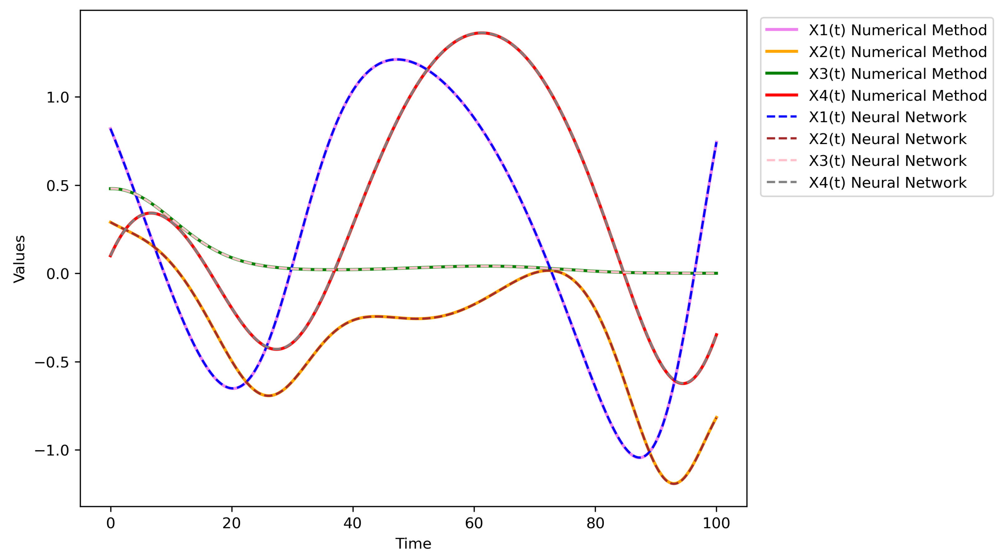
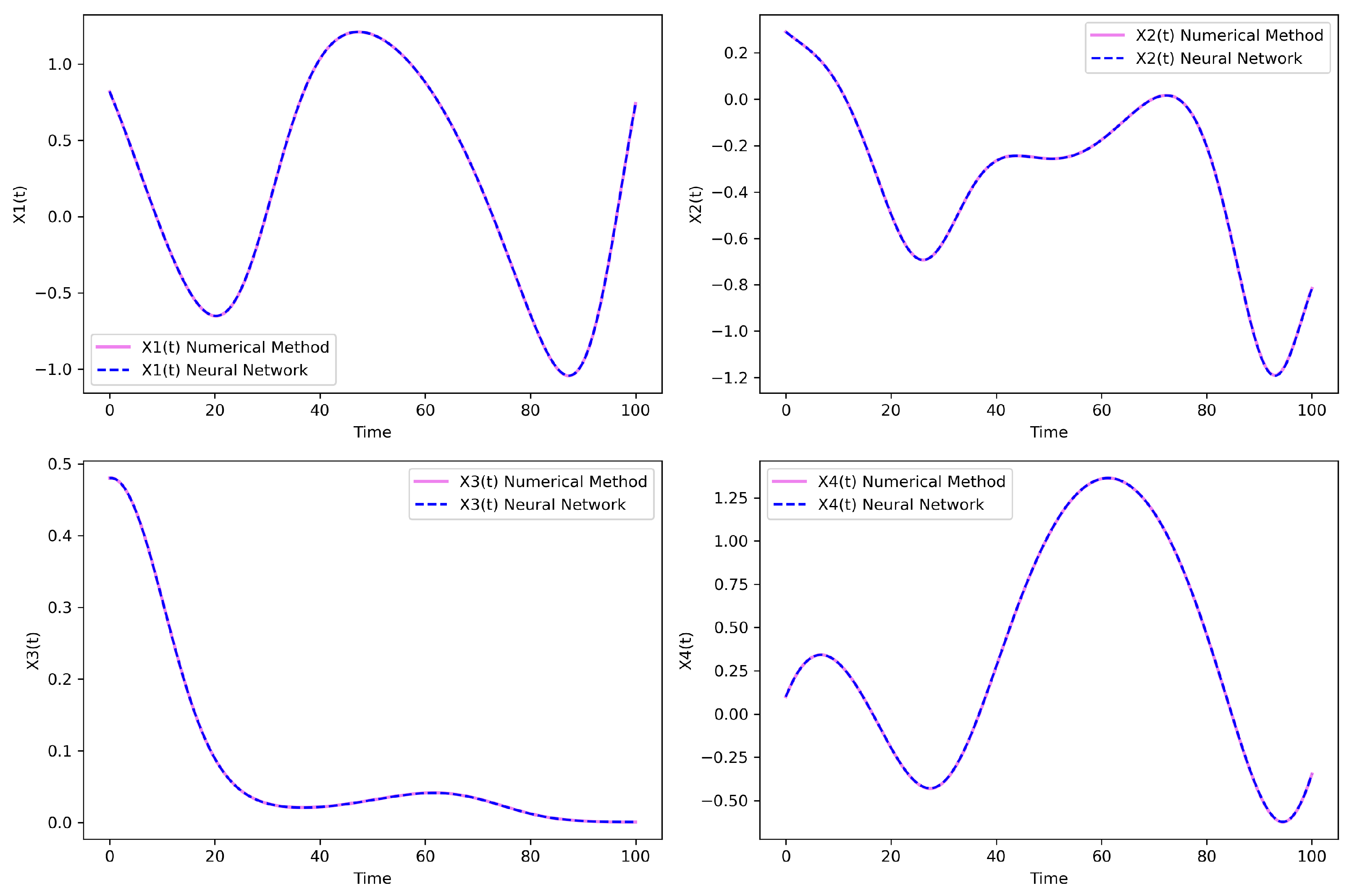
5. Results and Evaluation

In this study, we conducted an experiment to construct a neural network with an architecture consisting of an input layer that receives different time data points, 16 hidden layers with 100 neurons each, and an output layer with four neurons. The neurons in the output layer represent the time-dependent values of the four functions to be determined in the system of Equation (1). We set $\alpha =10$, $\beta =1$, and used the Adam optimizer [31,32] to minimize the loss function. The time interval $t=[0,100]$ was divided into N = 20,000 equally spaced time data points. For the numerical method, in this study, we use the SciPy library [34] to employ the RK45 method [35,36], which combines the fourth-order and fifth-order Runge-Kutta formulas to achieve high accuracy and efficiency. This method allows for the adaptive adjustment of step size to meet the required accuracy while optimizing computational time. We solved system (1) using the RK45 numerical method with an absolute tolerance of $1\times {10}^{-6}$ and a relative tolerance of $1\times {10}^{-3}$ over the same time domain with N time points as used by the neural network method. The solutions from both methods were then compared and evaluated. When using the neural network method, we applied a learning rate schedule, where the initial learning rate was set to $8\times {10}^{-5}$ and gradually reduced over the training epochs, with the minimum learning rate being $1\times {10}^{-6}$. After 175,000 epochs, Figure 2 shows the value of the loss function over the training epochs. We observed that the neural network method, with a simple network architecture in our experiment, began to provide solutions with accuracy comparable to the RK45 method for all four solutions sought, as presented in

Table 1. Comparing the accuracy of the results between the solutions obtained using the numerical method and those obtained using the neural network method.

Method	$\mathit{X}1\left(\mathit{t}\right)$ Error	$\mathit{X}2\left(\mathit{t}\right)$ Error	$\mathit{X}3\left(\mathit{t}\right)$ Error	$\mathit{X}4\left(\mathit{t}\right)$ Error
Numerical method	$3.16804\times {10}^{-8}$	$5.73393\times {10}^{-8}$	$7.70381\times {10}^{-10}$	$4.67541\times {10}^{-9}$
Neural network	$5.67513\times {10}^{-9}$	$2.43858\times {10}^{-9}$	$7.54885\times {10}^{-10}$	$3.10772\times {10}^{-9}$

and illustrated in Figure 3.

To conduct a comparative analysis of the error between two methods, we apply the finite difference method, supported by the NumPy library [30,31], to approximate the derivatives of these solutions with respect to the time variable t. Then, we substitute the solutions obtained from both methods into the original system of Equation (1). The MSE method is used to calculate the difference between the left-hand side and the right-hand side. The smaller the MSE value, the smaller the error between the two sides, indicating that the obtained solution better satisfies the original system of equations.

Additionally, the direct comparison of the errors between the solutions obtained from the two methods is performed and evaluated using the following metrics [37]: R-squared, MAE (Mean Absolute Error), MSE (Mean Squared Error), and RMSE (Root Mean Squared Error):

$$R^2=1-{\displaystyle \frac{{\sum }_{i=1}^N{(y_i-{\widehat{y}}_i)}^2}{{\sum }_{i=1}^N{(y_i-\overline{y})}^2}}$$

$$MAE={\displaystyle \frac{1}{N}}\sum _{i=1}^N|y_i-{\widehat{y}}_i|$$

$$MSE={\displaystyle \frac{1}{N}}\sum _{i=1}^N(y_i-{\widehat{y}}_i{)}^2$$

$$RMSE=\sqrt{{\displaystyle \frac{1}{N}}\sum _{i=1}^N{(y_i-{\widehat{y}}_i)}^2}$$

where $y_i$ is the solution value obtained using the numerical method.

${\widehat{y}}_i$ is the solution value obtained using the neural network method.

$\overline{y}$ is the average value of all the solution values obtained using the numerical method.

N is the number of time data points.

The comparison results between the methods, including the RK45 numerical method and the PINNs method, presented in

Table 2. A direct comparison between the solutions obtained using the numerical method and those obtained using the neural network method.

Evaluation Metric	$\mathit{X}1\left(\mathit{t}\right)$	$\mathit{X}2\left(\mathit{t}\right)$	$\mathit{X}3\left(\mathit{t}\right)$	$\mathit{X}4\left(\mathit{t}\right)$
R-squared	$0.99999843520$	$0.99999507773$	$0.99999921467$	$0.99999709511$
MAE	$0.00065521649$	$0.00064897482$	9.55051342325 × ${10}^{-5}$	$0.00093267431$
MSE	7.88852598020 × ${10}^{-7}$	6.61855514079 × ${10}^{-7}$	1.26016840498 × ${10}^{-8}$	1.17917245907 × ${10}^{-6}$
RMSE	$0.00088817374$	$0.00081354503$	$0.00011225722$	$0.00108589708$

and visualized in Figure 4 and Figure 5, demonstrate that the solutions obtained from these methods are equivalent.

6. Conclusions

In this study, we proposed a method using PINNs to solve a system of nonlinear differential equations describing the ESD system. Experimental results indicate that the PINNs method is a novel and effective approach. PINNs, a type of neural networks present several distinct advantages, such as providing solutions over a continuous domain and the ability to leverage the computational power of modern computers. The experimental results in this study show that PINNs achieve solutions comparable to the RK45 method. Furthermore, this approach demonstrates outstanding potential. According to general methods for improving and developing deep learning models, the performance of PINNs can be enhanced by adjusting the network architecture to be more complex (such as increasing the number of hidden layers and neurons in each layer), selecting or developing suitable optimization functions, as well as increasing the data and training time. These factors will help the model learn more complex representations, playing a crucial role in fully harnessing the power of PINNs. However, this comes at the cost of greater computational time and the need for a sufficiently powerful computing system. Moreover, ensuring the stability and convergence speed of the model is a significant challenge. While numerical methods have well-established mathematical theories that prove the stability and convergence of solutions, the evaluation of neural network-based approaches still mainly relies on empirical methods, which is a limitation. Overall, although this is a promising approach with high applicability in solving the nonlinear ESD system, there remain significant challenges, particularly in enhancing model stability, optimizing convergence speed, and reducing computational power requirements. However, we emphasize that neural network methods are not intended to be a complete replacement but rather a supplementary approach that can offer benefits when used alongside numerical methods in solving complex nonlinear problems, such as the one we are considering. Therefore, this research topic warrants further investigation in the future.

References

1. Chicone, C. Ordinary Differential Equations with Applications; Springer: New York, NY, USA, 1999. [Google Scholar]
2. Wong, P.J.Y. Applications of Partial Differential Equations; MDPI: Basel, Switzerland, 2023. [Google Scholar] [CrossRef]
3. Zachmanoglou, E.C.; Thoe, D.W. Introduction to Partial Differential Equations with Applications; Dover Publications, Inc.: New York, NY, USA, 1986. [Google Scholar]
4. Tomin, N.; Shakirov, V.; Kurbatsky, V.; Muzychuk, R.; Popova, E.; Sidorov, D.; Kozlov, A.; Yang, D. A multi-criteria approach to designing and managing a renewable energy community. Renew. Energy 2022, 199, 1153–1175. [Google Scholar] [CrossRef]
5. Sidorov, D.; Tao, Q.; Muftahov, I.; Zhukov, A.; Karamov, D.; Dreglea, A.; Liu, F. Energy balancing using charge/discharge storages control and load forecasts in a renewable-energy-based grids. In Proceedings of the 2019 Chinese Control Conference (CCC), Guangzhou, China, 27–30 July 2019; pp. 6865–6870. [Google Scholar] [CrossRef]
6. Sun, M.; Jia, Q.; Tian, L. A new four-dimensional energy resources system and its linear feedback control. Chaos Solitons Fractals 2007, 39, 101–108. [Google Scholar] [CrossRef]
7. Sun, M.; Tian, L.; Fu, Y. An energy resources demand–supply system and its dynamical analysis. Chaos Solitons Fractals 2005, 32, 168–180. [Google Scholar] [CrossRef]
8. Sun, M.; Tian, L.; Jia, Q. Adaptive control and synchronization of a four-dimensional energy resources system with unknown parameters. Chaos Solitons Fractals 2009, 39, 1943–1949. [Google Scholar] [CrossRef]
9. Vuik, C.; Vermolen, F.J.; van Gijzen, M.B.; Vuik, M.J. Numerical Methods for Ordinary Differential Equations; Delft University of Technology (TU Delft): Delft, The Netherlands, 2023. [Google Scholar] [CrossRef]
10. Lyengar, S.R.K.; Jain, R.K. Numerical Methods; New Age International Publishers: New Delhi, India, 2009. [Google Scholar]
11. Cybenko, G. Approximation by superpositions of a sigmoidal function. Math. Control Signal Syst. 1989, 2, 303–314. [Google Scholar] [CrossRef]
12. Hornik, K.; Stinchcombe, M.; White, H. Universal approximation of an unknown mapping and its derivatives using multilayer feedforward networks. Neural Netw. 1990, 3, 551–560. [Google Scholar] [CrossRef]
13. Lagaris, I.E.; Likas, A.; Fotiadis, D.I. Artificial Neural Networks for Solving Ordinary and Partial Differential Equations. IEEE Trans. Neural Netw. 1998, 9, 987–1000. [Google Scholar] [CrossRef]
14. Raissi, M.; Perdikaris, P.; Karniadakis, G.E. Physics-Informed Neural Networks: A Deep Learning Framework for Solving Forward and Inverse Problems Involving Nonlinear Partial Differential Equations. J. Comput. Phys. 2019, 378, 686–707. [Google Scholar] [CrossRef]
15. Raissi, M.; Perdikaris, P.; Karniadakis, G.E. Physics Informed Deep Learning (Part I): Data-driven Solutions of Nonlinear Partial Differential Equations. arXiv 2017, arXiv:1711.10561. [Google Scholar] [CrossRef]
16. Raissi, M.; Yazdani, A.; Karniadakis, G.E. Hidden Fluid Mechanics: A Navier-Stokes Informed Deep Learning Framework for Assimilating Flow Visualization Data. arXiv 2018, arXiv:1808.04327. [Google Scholar] [CrossRef]
17. Margenberg, N.; Hartmann, D.; Lessig, C.; Richter, T. A Neural Network Multigrid Solver for the Navier-Stokes Equations. J. Comput. Phys. 2022, 460, 110983. [Google Scholar] [CrossRef]
18. Hu, B.; McDaniel, D. Applying Physics-Informed Neural Networks to Solve Navier–Stokes Equations for Laminar Flow Around a Particle. Math. Comput. Appl. 2023, 28, 102. [Google Scholar] [CrossRef]
19. Farkane, A.; Ghogho, M.; Oudani, M.; Boutayeb, M. EPINN-NSE: Enhanced Physics-Informed Neural Networks for Solving Navier-Stokes Equations. arXiv 2023, arXiv:2304.03689. [Google Scholar] [CrossRef]
20. Eivazi, H.; Tahani, M.; Schlatter, P.; Vinuesa, R. Physics-Informed Neural Networks for Solving Reynolds-Averaged Navier–Stokes Equations. Phys. Fluids 2022, 34, 075117. [Google Scholar] [CrossRef]
21. Lu, L.; Meng, X.; Mao, Z.; Karniadakis, G.E. DeepXDE: A Deep Learning Library for Solving Differential Equations. SIAM Rev. 2021, 63, 208–228. [Google Scholar] [CrossRef]
22. Sidorov, D.; Tynda, A.; Muftahov, I.; Dreglea, A.; Liu, F. Nonlinear Systems of Volterra Equations with Piecewise Smooth Kernels: Numerical Solution and Application for Power Systems Operation. Mathematics 2020, 8, 1257. [Google Scholar] [CrossRef]
23. Yuan, L.; Ni, Y.-Q.; Deng, X.-Y.; Hao, S. A-PINN: Auxiliary Physics-Informed Neural Networks for Forward and Inverse Problems of Nonlinear Integro-Differential Equations. J. Comput. Phys. 2022, 462, 111260. [Google Scholar] [CrossRef]
24. Li, H.; Shi, P.; Li, X. Machine Learning for Nonlinear Integro-Differential Equations with Degenerate Kernel Scheme. Commun. Nonlinear Sci. Numer. Simul. 2024, 138, 108242. [Google Scholar] [CrossRef]
25. Matthews, J.; Bihlo, A. PinnDE: Physics-Informed Neural Networks for Solving Differential Equations. arXiv 2024, arXiv:2408.10011. [Google Scholar] [CrossRef]
26. Baty, H.; Baty, L. Solving Differential Equations Using Physics-Informed Deep Learning: A Hands-On Tutorial with Benchmark Tests. arXiv 2023, arXiv:2302.12260. [Google Scholar] [CrossRef]
27. Uriarte, C. Solving Partial Differential Equations Using Artificial Neural Networks. arXiv 2024, arXiv:2403.09001. [Google Scholar] [CrossRef]
28. Gorikhovskii, V.I.; Evdokimova, T.O.; Poletansky, V.A. Neural Networks in Solving Differential Equations. J. Phys. Conf. Ser. 2022, 2308, 012008. [Google Scholar] [CrossRef]
29. Goodfellow, I.; Bengio, Y.; Courville, A. Deep Learning; MIT Press: Cambridge, MA, USA, 2016. [Google Scholar]
30. Chollet, F. Deep Learning with Python, 2nd ed.; Manning Publications: Shelter Island, NY, USA, 2021. [Google Scholar]
31. Géron, A. Hands-On Machine Learning with Scikit-Learn, Keras, and TensorFlow, 2nd ed.; O’Reilly Media: Sebastopol, CA, USA, 2019. [Google Scholar]
32. Nielsen, M. Neural Networks and Deep Learning. 2016. Available online: http://neuralnetworksanddeeplearning.com/ (accessed on 15 October 2024).
33. Nguyen, T.T. Basic Deep Learning. 2020. Available online: https://nttuan8.com/sach-deep-learning-co-ban/ (accessed on 1 October 2024).
34. SciPy Reference. Available online: https://docs.scipy.org/doc/scipy/reference/integrate.html (accessed on 5 September 2024).
35. Dormand, J.R.; Prince, P.J. A Family of Embedded Runge-Kutta Formulae. J. Comput. Appl. Math. 1980, 6, 19–26. [Google Scholar] [CrossRef]
36. Shampine, L.W. Some Practical Runge-Kutta Formulas. Math. Comput. 1986, 46, 135–150. [Google Scholar] [CrossRef]
37. Wang, X.; Liu, X.; Wang, Y.; Kang, X.; Geng, R.; Li, A.; Xiao, F.; Zhang, C.; Yan, D. Investigating the Deviation Between Prediction Accuracy Metrics and Control Performance Metrics in the Context of an Ice-Based Thermal Energy Storage System. J. Energy Storage 2024, 91, 112126. [Google Scholar] [CrossRef]
Figure 1. Overview of the method, where ε is the desired value to be achieved when minimizing the loss function, and m a x is the maximum limit of the number of training epochs.
Computation 13 00013 g001
Figure 2. A chart describing the value of the loss function over the training epochs.
Computation 13 00013 g002
Figure 3. The chart visualizes a comparison of the accuracy of the two methods.
Computation 13 00013 g003
Figure 4. A general graph illustrating the direct comparison results between the RK45 numerical method and the neural network method.
Computation 13 00013 g004
Figure 5. A detailed graph illustrating the direct comparison results between the RK45 numerical method and the neural network method.
Computation 13 00013 g005