Bayesian Optimized Machine Learning Model for Automated Eye Disease Classification from Fundus Images

Abstract

Eye diseases are defined as disorders or diseases that damage the tissue and related parts of the eyes. They appear in various types and can be either minor, meaning that they do not last long, or permanent blindness. Cataracts, glaucoma, and diabetic retinopathy are all eye illnesses that can cause vision loss if not discovered and treated early on. Automated classification of these diseases from fundus images can empower quicker diagnoses and interventions. Our research aims to create a robust model, BayeSVM500, for eye disease classification to enhance medical technology and improve patient outcomes. In this study, we develop models to classify images accurately. We start by preprocessing fundus images using contrast enhancement, normalization, and resizing. We then leverage several state-of-the-art deep convolutional neural network pre-trained models, including VGG16, VGG19, ResNet50, EfficientNet, and DenseNet, to extract deep features. To reduce feature dimensionality, we employ techniques such as principal component analysis, feature agglomeration, correlation analysis, variance thresholding, and feature importance rankings. Using these refined features, we train various traditional machine learning models as well as ensemble methods. Our best model, named BayeSVM500, is a Support Vector Machine classifier trained on EfficientNet features reduced to 500 dimensions via PCA, achieving 93.65 ± 1.05% accuracy. Bayesian hyperparameter optimization further improved performance to 95.33 ± 0.60%. Through comprehensive feature engineering and model optimization, we demonstrate highly accurate eye disease classification from fundus images, comparable to or superior to previous benchmarks.

1. Introduction

Eye disease has always been a part of human history. It has been with us since we were born. As a result, the impact of eye disease on human health is immense. There are various eye diseases, such as cataracts, glaucoma, diabetic retinopathy, etc. [1]. A cataract is characterized by the clouding of the eye’s lens, appearing whitish from the outside [2]. The whiter the cataract, the more severe the condition, leading to blurred vision [3]. While most cases are age-related, cataracts can also occur due to injury or other medical conditions [3]. Diabetic retinopathy (DR), on the other hand, is a complication of diabetes that affects the blood vessels in the retina, resulting in vision problems and potential vision loss [4]. Glaucoma, the third condition under investigation, is caused by damage to the optic nerve, often due to increased intraocular pressure [5]. If left untreated, glaucoma can lead to irreversible vision loss and blindness [5]. These diseases directly impact the eyes and can blind a person forever [6]. It is estimated that approximately 2.2 billion people worldwide suffer from eye diseases or vision impairments, of which at least 1 billion can be prevented [6]. Currently, 3.5% of people between the ages of 40 and 80 have glaucoma [7]. In countries with limited resources, the incidence of glaucoma is rising along with life expectancies, and, by 2040, an estimated 112 million people will be affected [7].

Consequently, early diagnosis is crucial to halting the progression of these debilitating eye conditions. Typically, ophthalmic assistants and ophthalmologists examine fundus images to assess the eye’s condition and facilitate early diagnosis [8]. Through these fundus images, the central and peripheral retina, optic disc, and macula can be visualized, providing valuable insights into the presence and severity of the aforementioned eye diseases [9]. Machine learning (ML) techniques have emerged as powerful tools to enhance the capabilities [10] and efficiency of ophthalmic professionals [11], addressing various challenges in ophthalmic practices [12].

Recognizing this opportunity, our study aims to develop a robust and accurate ML model, BayeSVM500, specifically tailored for the automated classification of eye diseases from fundus images. By adopting a comprehensive approach that synergistically combines state-of-the-art deep learning (DL) models, intricate feature engineering techniques, and cutting-edge Bayesian optimization strategies, we strive to achieve superior classification performance that surpasses existing benchmarks. The proposed BayeSVM500 model represents a significant stride towards leveraging the full potential of artificial intelligence in the realm of ophthalmic diagnostics. By automating the disease classification process with unparalleled accuracy, our model has the potential to revolutionize healthcare delivery, enabling more efficient screening and earlier intervention and, ultimately, improving patient outcomes on a global scale. The main contributions of our research are the following:

• We developed a custom BayeSVM500 model for eye disease classification, combining Bayesian methods and Support Vector Machines.
• We evaluated five deep feature extraction techniques and selected EfficientNet as the optimal approach for our model.
• We explored five deep feature reduction and selection techniques, choosing PCA with 500 features as the best for our model.
• We achieved an accuracy of 95.33 ± 0.60% with our model, surpassing benchmarks and transfer learning models.

In the following sections, we delve into the intricate details of our methodology, encompassing image preprocessing, feature extraction, dimensionality reduction, and model training. We also present a comprehensive evaluation of our model’s performance, benchmarking it against existing state-of-the-art approaches and elucidating the key factors that contribute to its superior accuracy. Finally, we discuss the broader implications of our findings and outline future research directions, underscoring the immense potential of ML-driven solutions in mitigating the global burden of eye diseases.

2. Literature Review

Several studies have been conducted to explain how to classify eye diseases. This information helps us improve our diagnosis and understanding of the disease.

Babaqi T. et al. [13] developed a CNN model by using a pre-trained model architecture named EfficientNet for the four-class classification of eye disease. They also used the transfer learning model in their research. They collected around 4200 colored images from different sources like Kaggle, www5.cs.fau.de (accessed on 25 April 2024), and the Indian Diabetic Retinopathy Image Dataset (IDRiD). Their findings demonstrate that the transfer learning model performed better than their developed CNN model, where the transfer learning model achieved 94% accuracy, but their custom CNN models achieved only 84% accuracy. Bambang Krismono Triwijoyo et al. [14] implemented a DL approach for the classification of eye diseases based on color fundus images. In this research, they used a public STARE dataset, which contains 400 retinal color images and resized images in the preprocessing step for their 15 classes. They increased images to balance the dataset by using a random oversampling mechanism. They achieved 80.93% accuracy using CNN as a classifier for the classification of retinal images. The accuracy of this research was also very low. Omar Bernabé et al. [15] presented a novel intelligent pattern classification algorithm based on a convolutional neural network. They used two different datasets for the construction, training, and testing of the intelligent pattern classifier. They used 565 images of glaucoma and DR and achieved 99.89% accuracy. The dataset they used in their study contained only 565 images.

Sushma K Sattigeri et al. [16] built a DL model that distinguishes between a normal eye and a diseased eye. In their study, they discussed five eye diseases: conjunctivitis, cataracts, uveitis, bulging eyes, and crossed eyes. Utilizing digital image processing methods like segmentation, morphology, and convolution neural networks, they proposed a unique method to create an automated eye disease identification model using visually observable symptoms. They obtained 96% accuracy on single-eye images and 92.31% accuracy on two-eye images. Serhii Yaroshchak et al. [17] introduced the GMD model based on multi-label classification with additional techniques to detect and diagnose. They acquired a dataset from Kaggle, which contained 2050 images of glaucoma, diabetic retinopathy, myopia, and normal classes. They also collected data from iChallenge-GON Comprehension and Deep Convolutional Generative Adversarial Network (DCGAN). They developed a CNN model named the GMD model, which has a set of convolution layers, pooling layers, and fully connected layers. This model achieved 95% accuracy. They compared it with Alex, VGG16, and InceptionV3, but these gained 92%, 92%, and 94% accuracy, respectively. Using the relatively new DDR dataset, Paradisa R. H. et al. [18] present a DL method for DR fundus image classification using the concatenate model. They efficiently divided 13,673 fundus images into three groups: PDR, NPDR, and no DR. During the data preprocessing step, the dataset was first processed to create an image that the model could recognize more readily. They employed the Inception-ResNetV2 and DenseNet121 to concatenate the model for feature extraction by using MLP. Their suggested approach outperformed the others in terms of accuracy, which was 91%, with an average precision and recall for the F1-score coming in at 91% and 90%, respectively.

Ahmed M. R. [19] used a fully connected MATLAB deep convolutional neural network (DCNN) to train on fundus images with supervised learning using labeled healthy images and images of glaucoma disease. In their research, they used a variety of image processing techniques, including power transform, complement, B&W, grayscale, and resizing. The deep convolutional neural network texture feature extraction algorithm was used to extract features such as skewness, kurtosis, energy, contrast, correlation, homogeneity, entropy, mean, standard deviation, variance, and skewness (DCNN). A deep convolutional neural network with one hidden layer, sixteen input neurons, and two output neurons (indicating healthy or unhealthy states) achieved a detection accuracy of 92.78%. They only classified two classes.

Many previous studies, including Babaqi T. et al. [13], Bambang Krismono Triwijoyo et al. [14], Omar Bernabé et al. [15], and Serhii Yaroshchak et al. [17], grappled with smaller datasets, impacting the robustness of their models. We overcame this limitation by using a dataset of over 5000 fundus images from various sources, allowing for more accurate model training. Studies such as Babaqi T. et al. [13], Bambang Krismono Triwijoyo et al. [14], and Paradisa R. H. et al. [18] reported accuracy rates below 91%, indicating challenges in achieving precision. Our systematic approach, which employs advanced CNN architectures and efficient feature extraction, achieved an overall good accuracy. Ahmed M. R. [19] focused solely on classifying healthy and glaucoma states, missing the broader spectrum of eye diseases. We classified across four classes—cataract, diabetic retinopathy, glaucoma, and normal—providing a comprehensive analysis of diverse eye conditions. Prior studies, such as Babaqi T. et al. [13], did not conduct a systematic evaluation of dimensionality reduction techniques, potentially missing out on optimization opportunities. We systematically evaluated PCA over various feature counts, offering insights into the optimal balance between accuracy and efficiency. While Sushma K Sattigeri et al. [16] proposed a unique method, they lacked in-depth model interpretability. Leveraging attention maps, which highlight the important features the model focuses on during predictions, we provide both visual and quantitative explanations for our model’s decision-making process, enhancing trust in our automated disease screening system. Few studies, such as Serhii Yaroshchak et al. [17], compared their models with others, leaving gaps in the benchmarking process. We conducted a comprehensive comparative analysis, showcasing the advantages of our proposed BayeSVM500 model against transfer learning models and achieving superior performance. Our study bridges these gaps by offering a systematic and comprehensive approach to automated eye disease classification, contributing valuable insights to the field.

3. Methodology

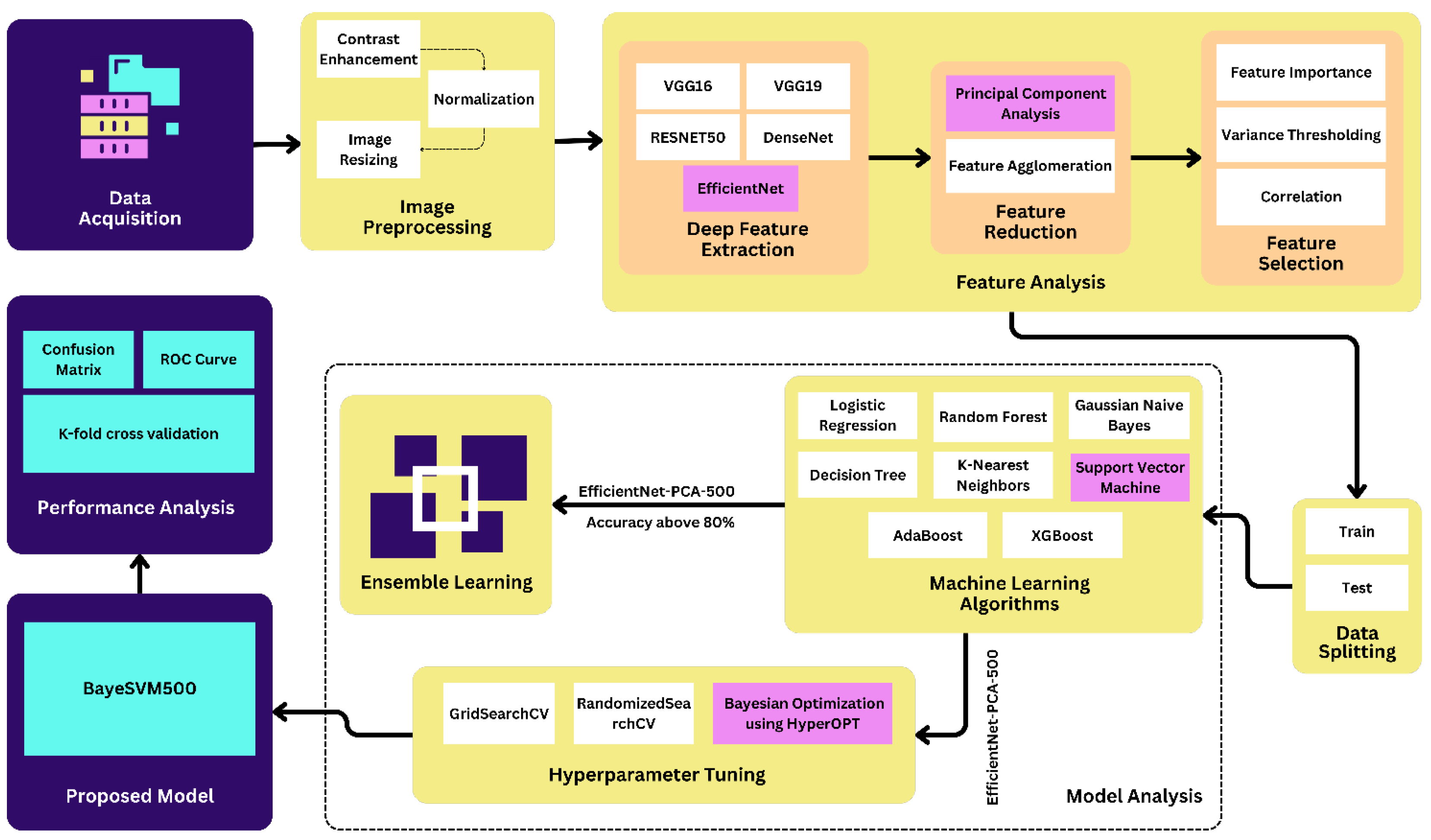
We implemented contrast enhancement, normalization, and image resizing techniques in the preprocessing step. After the preprocessing step, we applied deep feature extraction techniques using five different transfer learning algorithms such as VGG16, VGG19, ResNet50, EffcientNet, and DenseNet. Then, we applied the feature reduction and selection techniques on the features extracted from the datasets using PCA, feature agglomeration, correlation, variance thresholding, and feature importance techniques. We used eight popular ML algorithms in this study: LR, RF, GNB, DT, KNN, SVM, AdaBoost, and XGBoost. Figure 1 shows the proposed methodology of the eye disease classification studies.

3.1. Dataset Description

This study used six different datasets, which are shown in

Table 1. Dataset description.

Dataset	Cataract	DR	Glaucoma	Normal
eye_diseases_classification [20]	1038	1098	1007	1074
cataract dataset [21]	-	-	-	300
1000 Fundus images with 39 categories [9]	-	-	-	38
Disease Grading [22]	-	413	-	-
glaucoma dataset [23]	-	-	168	-
High-Resolution Fundus (HRF) Image Database [24]	-	15	15	15
Total = 5181	1038	1526	1190	1427

. The original dataset contains 4217 images, which were divided into four categories. The cataract, diabetic retinopathy, glaucoma, and normal classes have 1038, 1098, 1007, and 1074 images, respectively, which were collected from the site Kaggle [20]. We acquired three more datasets from Kaggle, containing 300 cataracts, 168 glaucoma, and 38 normal images [9,21,22]. Furthermore, we added 413 and 15 DR images from IEEE-Dataport and Pattern Recognition Lab, respectively, [23,24]. We also acquired 15 glaucoma and 15 normal images from the Pattern Recognition Lab [24]. Finally, we used 5181 images in this study where cataract, diabetic retinopathy, glaucoma, and normal class contained 1038, 1526, 1190, and 1427 images, respectively.

3.2. Image Preprocessing Techniques

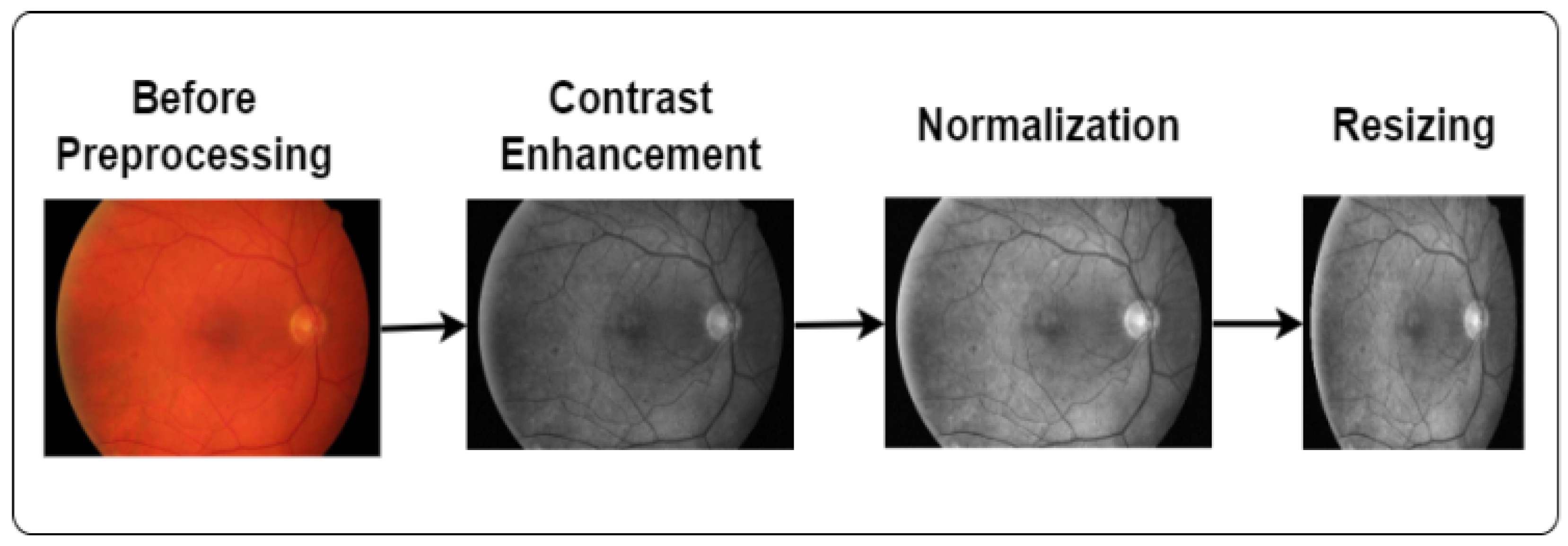
Image processing is a technique to convert low-quality images into high-quality images. It plays a vital role in enhancing the image quality and eliminating unwanted distortions. We applied contrast enhancement, normalization, and image-resizing techniques in this study, as demonstrated in Figure 2.

3.2.1. Enhance the Image

We used contrast enhancement to improve the image visually. Contrast enhancement is the process of enhancing the visual distinction of an image. It mainly brightens lighter areas and darkens darker regions. Our study used this technique to make the image more vibrant and clearer. In this study, we also applied CLAHE (Contrast-Limited Adaptive Histogram Equalization) and grayscale conversion techniques to enhance image quality. Grayscale helps to reveal hidden details and highlight contrast changes. Furthermore, CLAHE optimizes the contrast and creates visually improved images [25]. The equation of CLAHE [26] is as follows:

$$\beta ={\displaystyle \frac{M}{N}}\left(1+{\displaystyle \frac{\alpha }{100}}\left(S_{max}-1\right)\right)$$

(1)

Here, M, N, and $\alpha$ indicate the region size, grayscale value, and clip factor. This clip factor describes the addition of a histogram ranging between 0 and 100. The region size and clip limit initiate the CLAHE operation.

3.2.2. Normalization

Normalization is the process of scaling the features to a consistent range, usually between 0 and 1. We applied normalization because it provides standardized input, making it easier to learn the patterns of the model. The equation for calculating the Min–Max normalization is [27]

$$X_{\mathrm{normalized}}=X-{\mathrm{X}}_{min}/X_{\max }-X_{\min }$$

(2)

Here, X is the original feature value, $X_{min}$ refers to the minimum, and $X_{max}$ refers to the maximum value of the feature.

3.2.3. Image Resizing

Image resizing is a common preprocessing technique in DL. It is the process of changing the image size [28]. We applied this technique because the size of all images was not the same. To ensure that a DL model can handle all inputs consistently, resizing the images to a fixed size can be useful. In this study, we resized all the images into a size of 224 × 224 [29].

3.3. Deep Feature Extraction

Feature extraction is a critical technique in the process of transforming raw data into numerical features [30]. It helps to capture patterns and information from the input image for further analysis [30]. In this study, we applied deep feature extraction techniques using some well-known transfer learning algorithms. Transfer learning algorithms offer a powerful solution for feature extraction due to their ability to learn complex patterns and representations from large datasets. In this research, we used VGG16, VGG19, ResNet50, EfficientNet, and DenseNet to extract the deep feature where VGG16 and VGG19 collected 4096 feature data and ResNet50, EfficientNet, and DenseNet collected 2048, 1280, and 1024 feature data, respectively [31]. The utilization of multiple architectures improved the research by offering a comprehensive understanding of how various models capture and represent information.

3.4. Feature Analysis

In this study, we conducted feature selection and reduction to analyze deep features. We applied PCA, feature agglomeration, correlation, variance thresholding, and feature importance techniques.

3.4.1. Feature Reduction

For feature reduction, we leveraged two techniques—PCA and feature agglomeration techniques [32]. PCA is an efficient dimensionality reduction technique that constructs relevant features using linear combinations of the original features [33]. It helped capture the most useful information from the high-dimensional deep features. Feature agglomeration groups similar features to reduce dataset complexity while maintaining crucial information [34].

3.4.2. Feature Selection

We applied three feature selection techniques—correlation-based feature selection [35], variance thresholding [36], and feature importance [37]. Correlation-based selection eliminates features that have a low correlation with the target variable, as those are less useful for prediction [35]. Variance thresholding removes features whose variance falls below a threshold, reducing noisy or invariant features [36]. Finally, feature importance assigns a score to each input feature based on how useful it is at predicting the target, allowing us to select impactful features [37]. The use of these techniques allowed the selection of the most informative features for model building.

3.5. Splitting Dataset

We divided the dataset into training and test subsets for model training and evaluation. The training set, containing 80% of the data (4144 images), was used to train the model. The remaining 20% (1037 images) was held out as the testing set to assess the model’s performance on unseen data. While we experimented with multiple data splits, we found that the 80:20 ratio consistently provided the best results in terms of model stability and accuracy.

3.6. Model Analysis

In this study, we applied eight machine-learning models and combined the top five models into six ensemble models. The eight ML models were LR, RF, GNB, DT, KNN, SVM, AdaBoost, and XGBoost. Finally, we applied hyperparameter tuning.

3.6.1. Machine Learning Model

Initially, we applied 8 ML and ensemble algorithms—LR, RF, GNB, DT, KNN, SVM, AdaBoost, and XGBoost on all 30 datasets. Based on the accuracy results above 80%, we narrowed down to the 5 top performing algorithms—LR, RF, KNN, SVM, and XGBoost. Among them, SVM achieved the highest accuracy. We extracted features using EfficientNet and applied PCA for dimensionality reduction to 100 features. To determine the optimal number of features, we evaluated PCA with 50, 100, 250, 500, 800, and 1000 features. A total of 500 PCA features applied on EfficientNet gave the best accuracy.

3.6.2. Ensemble Learning Model

In our first approach, we combined the top 5 algorithms into six ensemble models—LR + RF, LR + KNN, LR + SVM, LR + XGBoost, RF + XGBoost, and SVM + XGBoost. We evaluated these models before and after applying PCA feature reduction. The SVM + XGBoost ensemble achieved the highest accuracy after PCA in just 28 s, outperforming pre-PCA ensembles. Though the accuracy decreased slightly compared to PCA-SVM alone, the ensemble model provided a good trade-off between accuracy and efficiency.

3.6.3. Hyperparameter Tuning

In the second approach, we applied hyperparameter tuning on the SVM using GridSearchCV, RandomizedSearchCV, and Bayesian Optimization with the HyperOpt library. We tuned the parameter C and found the optimal value to be 6.592, and, for the parameter kernel, the optimal value was rbf. For this outcome, we conducted 50 trials and used 5-fold cross-validation. The optimal hyperparameter values identified by Bayesian Optimization resulted in the highest accuracy among all techniques.

3.7. Proposed Model

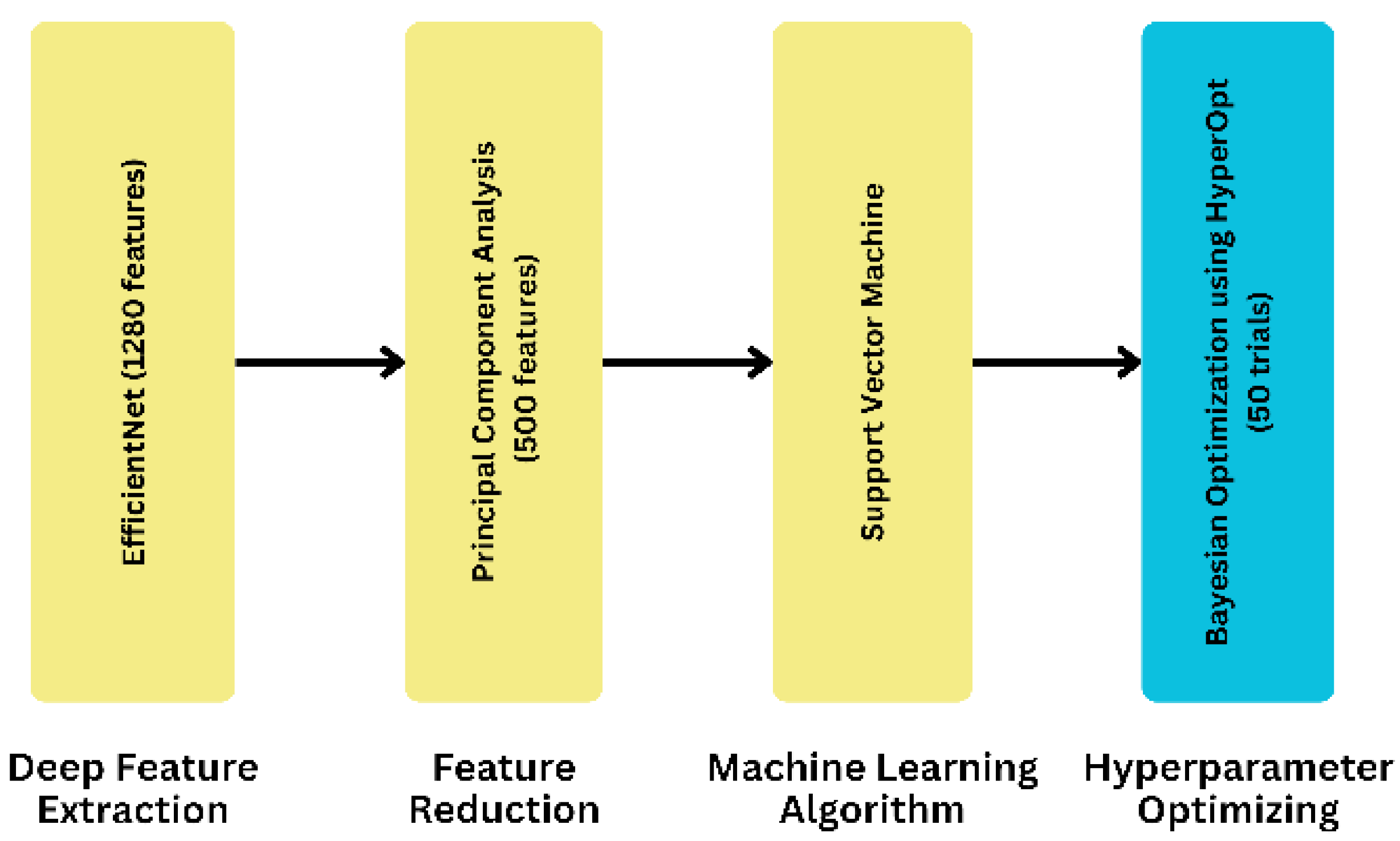
To develop our proposed model, we took a systematic approach by utilizing eight different ML algorithms, five different feature extraction techniques, and analyzing three feature selection and two feature reduction techniques, evaluating the five combinations of the best ML algorithms as ensemble methods, and leveraging three separate hyperparameter tuning search techniques. As for the final dataset, we selected it after applying the ML algorithms to compare its accuracy. The result led us to finalize the EfficientNet as a feature extraction technique. On the contrary, PCA is a feature reduction technique with a feature value of 500. In our proposed model, we used an SVM as the final ML algorithm to evaluate the dataset. In this case, we used C and kernel as parameters. We obtained the parameter value by using HyperOpt for the Bayesian optimization search technique. To get the best parameter value, we used 50 as the trial number. This provided the highest accuracy, demonstrating the effectiveness of our proposed approach. We have illustrated the process of obtaining our proposed model in Figure 3.

4. Experiments and Outcome Analysis

We applied several comparison-based experiments on all techniques from which we obtained our feature-extracted, reduced, and selected datasets. We conducted these experiments to build our proposed model by doing a comparative analysis using ML models between the techniques. We employed various metrics to evaluate model performance:

Accuracy indicates the general measurement of the model’s correctness. Accuracy is calculated using the following formula [38]:

$$Accuracy={\displaystyle \frac{TruePositives+TrueNegatives}{Totalobservations}}$$

(3)

Precision indicates how many of the predicted positive instances are positive. Precision is calculated using the following formula [39]:

$$Precision={\displaystyle \frac{TruePositives+TruePositives}{FalsePositives}}$$

(4)

Recall indicates the ability of the model to capture all the positive instances. Recall is calculated using the following formula [40]:

$$Recall={\displaystyle \frac{TruePositives+TruePositives}{FalseNegatives}}$$

(5)

F1-score indicates the harmonic mean of precision and recall, which provides a balance between precision and recall. F1-score is calculated using the following formula [41]:

$$F1score=2\times {\displaystyle \frac{Precision\times Recall}{Precision+Recall}}$$

(6)

In this study, we also calculate the mean, variance, and standard deviation to analyze and present the data comprehensively. The formulas for the mean, variance, and standard deviation are [42]

$$Mean={\displaystyle \frac{{\sum }_{i=1}^n{x}_i}{n}}$$

(7)

$$Variance={\displaystyle \frac{{\sum }_{i=1}^n{\left(x_i-Mean\right)}^2}{n-1}}$$

(8)

$$StandardDeviation=\sqrt{Variance}$$

(9)

These equations detail the calculation of key statistical measures such as mean, variance, and standard deviation used to analyze data distributions. The mean is determined by summing all individual data points $x_i$ and dividing by the total number of observations n. Variance quantifies the spread of the data by calculating the average of the squared differences between each data point and the mean, adjusted by dividing by $n-1$ to correct for sample size bias. Finally, the standard deviation, obtained as the square root of the variance, provides an understanding of the data’s dispersion around the mean in the same units as the data itself.

4.1. Experiments with Features

Our dataset is an image dataset. As a result, for our following approach, we need to know the features of each disease. So, we performed various feature extraction, feature reduction, and feature selection techniques to find the best features to acquire the best result.

4.1.1. Experiments on Feature Extraction Techniques

We evaluated five different DL models—VGG16, VGG19, ResNet50, EfficientNet, and DenseNet—for extracting features from the fundus images.

Table 2. Comparison between deep feature extraction models using ML models.

Algorithm	VGG16 (4096 Features) %	VGG19 (4096 Features) %	RESNET50 (2048 Features) %	EfficientNet (1280 Features) %	DenseNet (1024 Features) %
LR	86.02 ± 0.90	88.04 ± 0.85	85.54 ± 0.95	88.24 ± 0.80	84.67 ± 0.88
RF	81.77 ± 1.10	82.84 ± 1.20	84.57 ± 0.85	83.32 ± 1.10	85.82 ± 0.95
DT	68.76 ± 1.30	67.79 ± 1.40	75.41 ± 1.10	70.78 ± 1.20	78.50 ± 1.25
KNN	81.97 ± 1.05	83.90 ± 0.95	82.16 ± 1.15	80.91 ± 1.15	83.22 ± 1.10
SVM	85.25 ± 0.85	87.37 ± 0.90	85.15 ± 0.92	85.25 ± 0.88	84.47 ± 0.85
GNB	67.21 ± 1.40	69.53 ± 1.25	72.52 ± 1.15	69.43 ± 1.30	72.03 ± 1.20
Ada Boost	69.91 ± 1.15	73.48 ± 1.35	80.04 ± 0.85	75.60 ± 0.95	79.85 ± 0.90
XGBoost	85.82 ± 0.80	86.21 ± 0.75	88.04 ± 0.90	89.10 ± 0.85	89.39 ± 0.78

compares the classification accuracy achieved when training various ML algorithms on the extracted feature sets.

Among the feature extraction techniques, EfficientNet features achieved the highest accuracy of 89.39 ± 0.78% when classified using the XGBoost algorithm. This suggests EfficientNet’s effectiveness in capturing relevant representations from the eye disease images compared to other models like VGG and ResNet. Across the ML classifiers, XGBoost, SVM, and LR consistently performed well, with accuracies above 85% for multiple feature extractors. This indicates their suitability for this classification task. In contrast, models like GNB and DT showed comparatively lower performance. Overall, the best accuracy of 89.39 ± 0.78% was obtained using XGBoost on DenseNet features. However, EfficientNet matched closely at 89.10 ± 0.85% accuracy, making it a strong choice as a deep feature extractor, given its efficiency.

4.1.2. Experiments on Feature Reduction and Selection Techniques

After applying feature extraction techniques, we used five different types of feature reduction and feature selection techniques on each dataset. These techniques are called PCA, variance thresholding, feature agglomeration, correlation-based feature selection, and feature importance using RF. We performed this experiment because we wanted to determine if the reduced feature could also provide us with the same result or better.

The supplementary material includes detailed results from five additional experiments. We have moved these tables there to keep the main text more concise.

From these five experiments based on different types of feature reduction and feature selection techniques, we concluded that, after using EfficientNet and DenseNet individually on the dataset of PCA feature extraction technique, we obtained the highest accuracy, which was 88.91 ± 1.38%.

Performing PCA on both EfficientNet and DenseNet with 500 samples yielded improved results compared to the previous experiment with 100 features. The EfficientNet model demonstrated superior performance, achieving an accuracy of 93.65 ± 1.05%, as shown in

Table 3. Accuracy comparison after applying PCA with 500 features.

Algorithm	EfficientNet (500 Features) %	DenseNet (500 Features) %
LR	84.96 ± 1.25	84.57 ± 1.30
RF	78.11 ± 1.50	79.94 ± 1.40
DT	68.37 ± 1.75	68.95 ± 1.70
KNN	83.51 ± 1.10	87.46 ± 1.15
SVM	93.65 ± 1.05	89.59 ± 1.20
GNB	49.57 ± 2.65	56.51 ± 2.10
AdaBoost	73.19 ± 1.55	70.20 ± 1.60
XGBoost	85.73 ± 1.20	85.92 ± 1.25

, surpassing all previous outcomes.

In

Table 4. Comparison of EfficientNet accuracy with PCA applied at various feature dimensions.

Algorithm	EfficientNet (50 Features) %	EfficientNet (100 Features) %	EfficientNet (250 Features) %	EfficientNet (500 Features) %	EfficientNet (800 Features) %	EfficientNet (1000 Features) %
LR	83.70 ± 1.20	85.92 ± 1.15	86.50 ± 1.10	84.96 ± 1.25	87.75 ± 1.30	87.37 ± 1.18
RF	80.62 ± 1.50	82.35 ± 1.40	80.33 ± 1.35	78.11 ± 1.60	76.18 ± 1.55	77.92 ± 1.45
DT	69.91 ± 2.45	69.62 ± 2.05	69.53 ± 1.95	68.37 ± 2.10	66.83 ± 2.15	66.15 ± 2.20
KNN	82.93 ± 1.10	83.12 ± 1.12	82.84 ± 1.08	83.51 ± 1.15	83.41 ± 1.13	83.51 ± 1.10
SVM	87.75 ± 1.05	88.91 ± 1.08	91.97 ± 1.10	93.65 ± 1.02	89.78 ± 1.12	89.87 ± 1.15
GNB	70.30 ± 2.50	63.74 ± 2.75	54.25 ± 2.80	49.57 ± 2.85	48.60 ± 2.90	47.93 ± 2.95
Ada Boost	72.71 ± 1.80	74.64 ± 1.75	74.83 ± 1.70	73.19 ± 1.85	68.18 ± 2.35	71.75 ± 1.90
XGBoost	86.79 ± 1.25	86.89 ± 1.20	86.02 ± 1.18	85.73 ± 1.22	85.15 ± 1.30	84.86 ± 1.28

, we executed this experiment by changing the feature number of the PCA reduction technique. We compare all the results to obtain a better feature number to apply our proposed model. Our main aim was to take fewer features but obtain better results. As a result, we input six different feature numbers to check the accuracy. As shown in Table S1 of the supplementary material, we obtain the highest result for 100 feature numbers, 88.91 ± 1.38%, after applying SVM. Then, in Table 3, we obtain the highest value, 93.65 ± 1.05%, when the feature number is 500 after using SVM. To justify this feature number, we took a number of the features below and above 500. So, we took 50, 100, 250, 500, 800, and 1000 as feature values and showed the comparison among them.

All of the above experiments led us to identify the best extraction and reduction technique for our dataset, which is the EfficientNet feature extraction technique combined with PCA feature reduction. After extracting our dataset’s features using EfficientNet, we achieved the best accuracy by performing PCA, with the feature number set to 500, resulting in an impressive accuracy of 93.65 ± 1.05%.

EfficientNet is a state-of-the-art CNN architecture that stands out due to its unique compound scaling method, which balances the network’s depth, width, and resolution in a coordinated manner. This balanced approach leads to significantly higher performance and efficiency compared to other models that typically scale only one or two dimensions. EfficientNet’s architecture starts with a simple yet highly efficient baseline network, which is then scaled up using the compound scaling method. This ensures that the network maintains optimal performance without becoming overly complex. Additionally, EfficientNet uses advanced techniques like the Swish activation function and depthwise separable convolutions, which further enhance its performance and efficiency. The superior accuracy of EfficientNet, combined with its fewer parameters and reduced computational cost, makes it highly efficient for deployment on resource-constrained devices [43]. Its ability to maintain high accuracy while being computationally efficient was the primary reason for choosing EfficientNet over other architectures like VGG16, VGG19, ResNet50, and DenseNet. The integration of EfficientNet with PCA allowed us to effectively reduce the dimensionality of our dataset while preserving essential features, leading to a highly accurate and efficient model.

4.2. Experiments with Models

In this research, we conducted some experiments to achieve our goal. First, we built some ensemble learning models using those ML models, which gained over 80% accuracy. Then, we changed some parameters of our proposed model in the hyperparameter tuning section. We also compared our proposed model with some renowned transfer learning models. Finally, we analyzed the performance of BayeSVM500.

4.2.1. Performance Analysis Using Ensemble Model

In

Table 5. Performance of different algorithms before and after feature reduction.

Algorithms before Feature Reduction (1280 Features)	Performance %	Algorithms after Feature Reduction Using PCA (500 Features)	Performance %
Above 80% (LR + RF + KNN + SVM + XGBoost)	88.00 ± 2.00 (1 m 38 s ± 5 s)	Above 80% and 83% (LR + KNN + SVM + XGBoost)	89.00 ± 1.00 (37 s ± 2 s)
Above 83% (LR + RF + SVM + XGBoost)	88.00 ± 1.00 (1 m 33 s ± 4 s)	Above 85% (SVM + XGBoost)	91.00 ± 1.00 (28 s ± 2 s)
Above 85% (LR + SVM + XGBoost)	89.00 ± 1.00 (1 m 23 s ± 3 s)	—	—
Above 87% (LR + XGBoost)	89.00 ± 1.00 (1 m 19 s ± 3 s)	—	—

, we compare the accuracy and execution time of various ensemble learning models before and after applying PCA feature reduction on the EfficientNet feature-extracted dataset. The ensemble models are created by combining different algorithms based on accuracy thresholds: above 80%, above 83%, above 85%, and 87%. After applying PCA feature reduction, reducing the features from 1280 to 500, the execution time is significantly reduced compared to the models without feature reduction. The highest accuracy of 91 ± 1 % is achieved by the ensemble model combining SVM and XGBoost, with an execution time of only 28 s. This is a significant improvement compared to the 88 ± 2 % accuracy achieved by the ensemble model with all algorithms above the 80% threshold, which took 1 min and 38 s without feature reduction. The table demonstrates the effectiveness of ensemble learning models, especially when combined with feature reduction techniques like PCA, in achieving high accuracy while reducing computational time.

4.2.2. Performance Analysis Using Hyperparameter Tuning

For hyperparameter tuning, we used three search techniques, GridSearchCV, RandomizedSearchCV, and Bayesian Optimization techniques, on the SVM algorithm. The two parameters that we used in all three search techniques were C and kernel. For the Bayesian optimization technique, we obtained the best accuracy, which was 95.33%. In the Bayesian optimization search technique, we used HyperOPT to use the best-optimized parameter value and 50 trials to gain the output. We have illustrated the comparison of accuracy between different hyperparameter tuning techniques in Figure S1 of the supplementary file. Figure S2 of the supplementary file illustrates the improvement in test accuracy achieved by our proposed methodology using the SVM classifier on features extracted from the EfficientNet model. As shown in Figure S2 of the supplementary file, when using the full 1280 feature set from EfficientNet, the test accuracy was 85.25%. However, by applying PCA for dimensionality reduction and selecting an optimal number of features, we could significantly boost the classification performance. The progressive increase in test accuracy from 85.25% to 95.33% demonstrates the efficacy of our proposed approach—leveraging deep feature extraction, feature reduction, and hyperparameter optimization. This comprehensive methodology enabled the development of a high-performing BayeSVM500 model for automated eye disease classification from fundus images.

4.2.3. Comparison with Transfer Learning Model

This study showed that our proposed model performed better than the transfer learning models. These transfer learning models were applied to the fundus image dataset after following the preprocessed steps. All eight models produced low accuracy, less than 64%, with the lowest accuracy observed from ResNet152V2 at approximately 27.31 ± 2.50%. The accuracy of the remaining models lay between 27% and 64%. On the contrary, our proposed model, BayeSVM500, performed significantly better, achieving 95.33 ± 0.60% accuracy. Additionally, BayeSVM500 showed the highest performance in terms of precision, recall, and F1-score, with values of 96.13 ± 0.65%, 95.67 ± 0.58%, and 95.90 ± 0.60%, respectively. Furthermore, the training accuracy and validation accuracy of BayeSVM500 were 97.50 ± 0.50% and 96 ± 1%, respectively, indicating its robustness.

Table 6. Performance comparison with transfer learning models.

Models	Training Accuracy %	Validation Accuracy %	Testing Accuracy %	Precision %	Recall %	F1-Score %
VGG16	88.50 ± 1.50	70.00 ± 2.00	63.65 ± 2.30	72.15 ± 2.10	81.40 ± 1.80	76.46 ± 1.90
VGG19	86.75 ± 1.75	65.30 ± 2.50	52.02 ± 2.70	65.38 ± 2.60	70.25 ± 2.40	67.75 ± 2.50
InceptionV3	84.00 ± 2.00	55.00 ± 3.00	34.52 ± 2.50	48.21 ± 2.30	55.90 ± 2.60	51.81 ± 2.55
Xception	82.10 ± 2.10	52.75 ± 2.80	28.56 ± 2.70	42.75 ± 2.40	59.10 ± 2.50	49.46 ± 2.60
DenseNet201	87.50 ± 1.80	67.50 ± 2.40	52.69 ± 2.60	69.40 ± 2.30	75.85 ± 2.20	72.49 ± 2.35
EfficientNetV2L	83.00 ± 2.00	60.00 ± 3.00	30.96 ± 2.40	45.60 ± 2.50	62.45 ± 2.70	52.75 ± 2.60
ResNet152V2	81.00 ± 2.00	53.00 ± 3.00	27.31 ± 2.50	41.15 ± 2.40	65.20 ± 2.30	50.76 ± 2.45
MobileNetV2	85.00 ± 2.00	58.00 ± 3.00	35.96 ± 2.40	51.35 ± 2.30	57.40 ± 2.50	54.22 ± 2.40
BayeSVM500	97.50 ± 0.50	96.00 ± 1.00	95.33 ± 0.60	96.13 ± 0.65	95.67 ± 0.58	95.90 ± 0.60

presents a detailed comparison of the training accuracy, validation accuracy, testing accuracy, precision, recall, and F1-score for the transfer learning models and our proposed model.

4.2.4. Comparison of Results Across Multiple Data Splits

In Figure S3 of the supplementary file, we evaluate different data split ratios—80:20, 70:30, 65:35, and 60:40—using our dataset, which consisted of a total of 5181 images. The 80:20 split, which allocates 4144 images for training and 1037 images for testing, achieves the highest accuracy of 95.33%. In comparison, the other splits yield lower accuracies: 92.21% for the 70:30 split, 91.05% for the 65:35 split, and 88.78% for the 60:40 split. The superior performance of the 80:20 ratio is attributed to its optimal balance, providing sufficient data for both training and testing. This balance helps ensure that the model is well trained while still being evaluated on a sufficiently large test set, leading to more reliable and consistent results. Conversely, using a smaller proportion of data for training and a larger proportion for testing can lead to several issues. With less training data, the model may not learn effectively, resulting in underfitting. Underfitting occurs when the model fails to capture the underlying patterns in the training data due to its limited exposure. As a result, even though the test set is larger, the model’s performance on unseen data may be poorer because it has not been adequately trained. This imbalance between training and testing data can thus lead to less accurate and less reliable model performance.

4.3. Performance Analysis of BayeSVM500

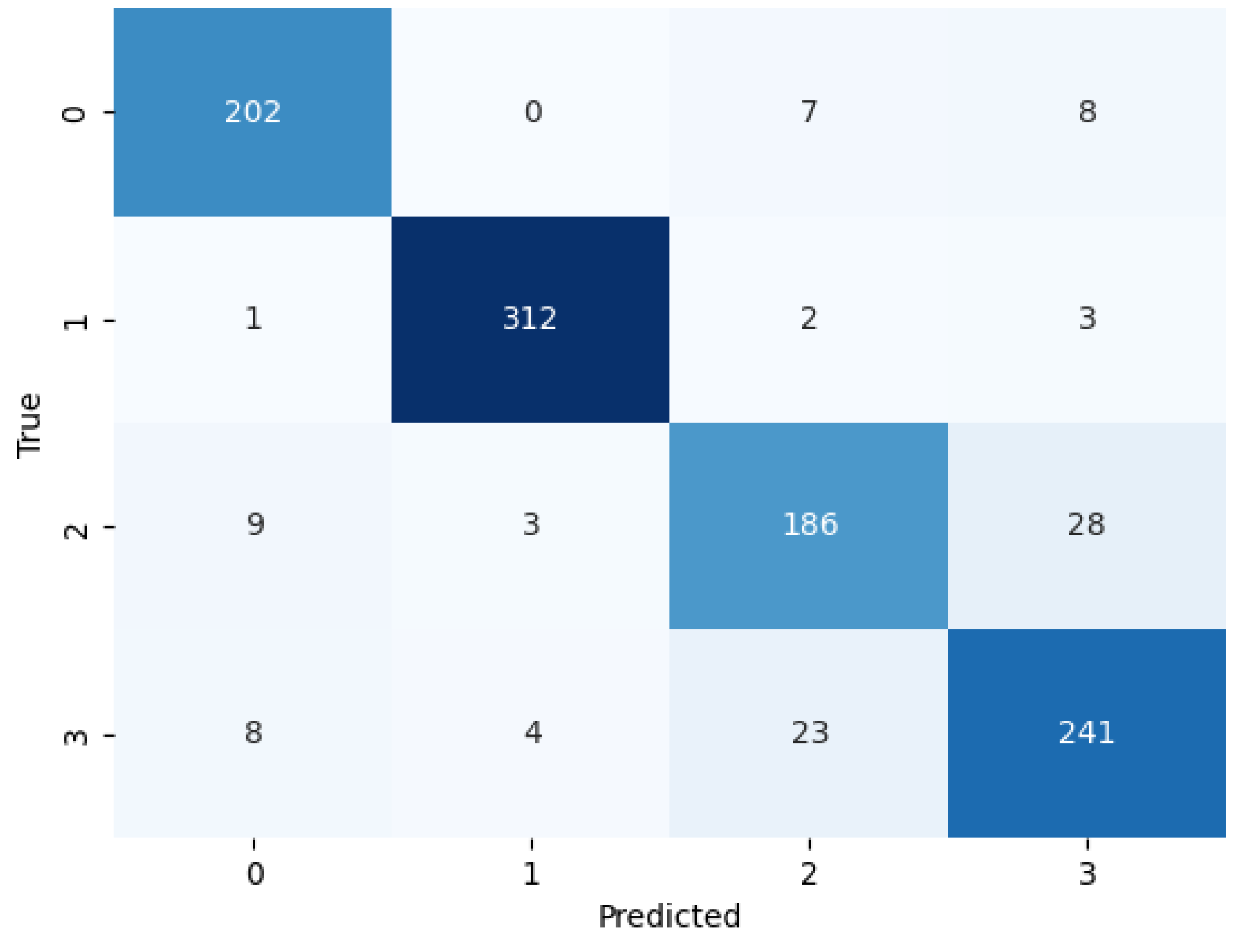
We evaluated the performance of BayeSVM500 using a confusion matrix, ROC curve, and k-fold cross-validation. The confusion matrix heatmap in Figure 4 provides insights into the model’s predictions across the four classes. The rows correspond to the true class labels, and the columns represent the predicted classes [44]. The diagonal elements represent the true positive predictions for each class—202 for class 0 (cataract), 312 for class 1 (diabetic_retinopathy), 186 for class 2 (glaucoma), and 241 for class 3 (normal). The low values in the off-diagonal elements indicate few false positive and false negative predictions. This demonstrates the model’s ability to consistently and accurately classify eye disease images without significant bias towards any particular class.

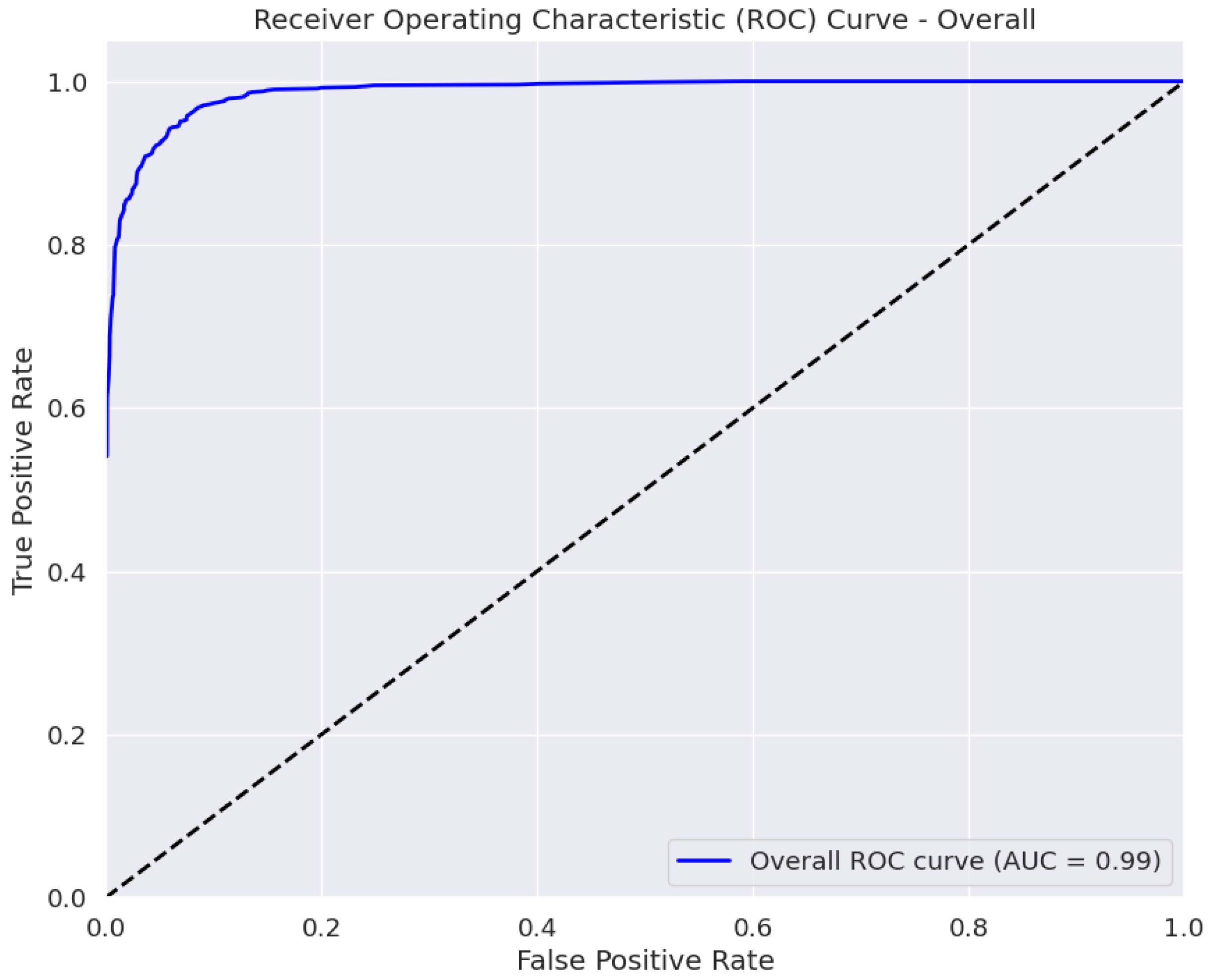
The AUC is a measure of the classifier’s ability to distinguish between classes, with a higher AUC value indicating better performance [45]. The ROC curve in Figure 5 plots the true positive rate against the false positive rate at various classification thresholds. The area under the curve (AUC) of 0.99 ± 0.01 indicates the excellent performance of our model in distinguishing between the four eye disease classes. Thus, BayeSVM500 demonstrates a high capability to accurately differentiate cataracts, diabetic retinopathy, glaucoma, and normal eye conditions.

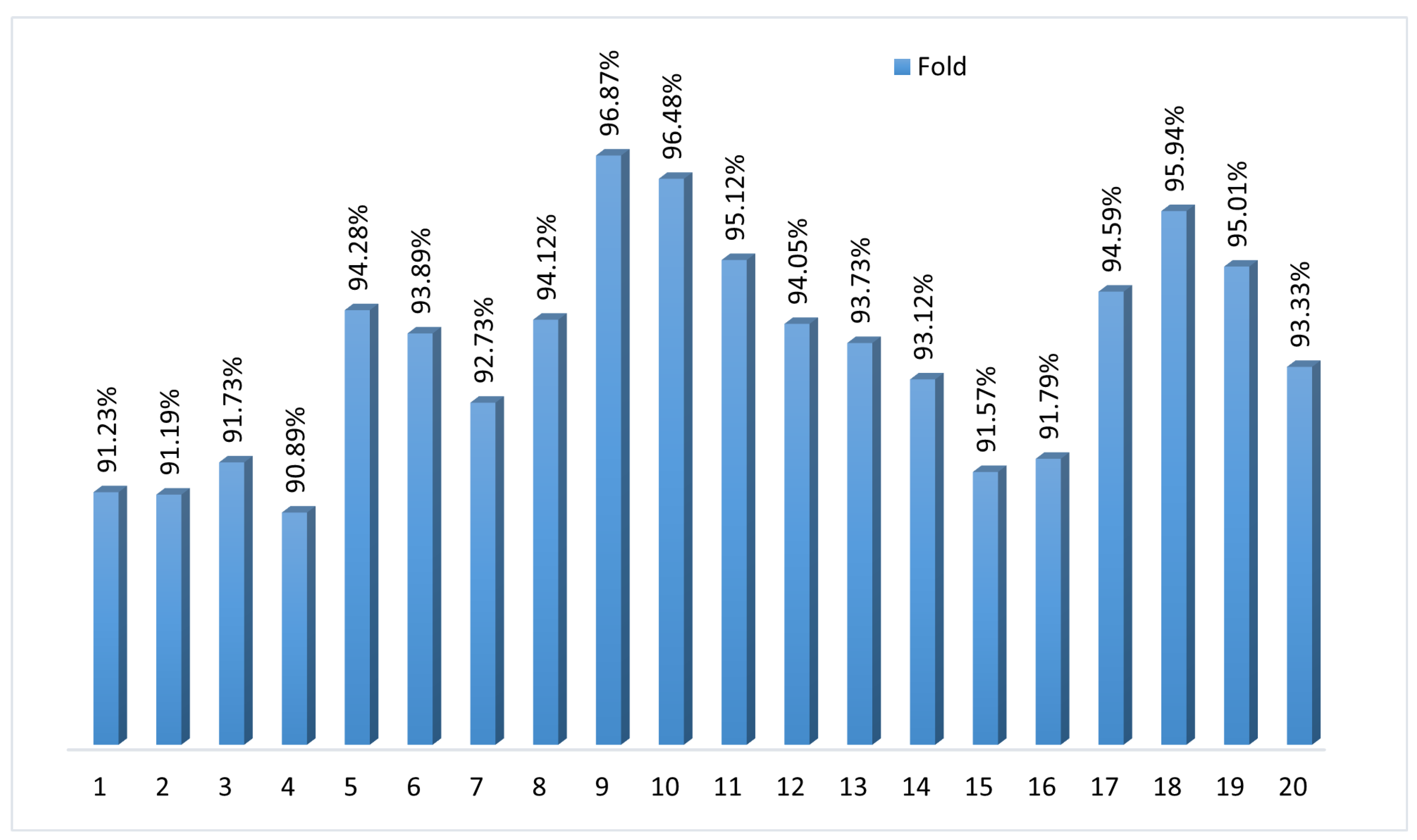
To assess the consistency and generalization performance, we applied k-fold cross-validation with k = 20. Figure 6 shows the accuracy scores for each fold ranging from 90.89% to 96.87%, with a mean accuracy of 93.59%. The narrow spread highlights how the model maintains stability and predictive power across different data subsets. The k-fold cross-validation validates BayeSVM500’s robustness in accurately classifying previously unseen fundus images. The consistently high accuracy demonstrates the model’s reliable performance in automated eye disease screening.

The model achieved an average accuracy of 94.02% across 20 folds, with a standard deviation of ±1.82. This indicates that the model’s performance was consistent, with most accuracy values falling within ±1.82 of the average.

4.4. Impact of Sample Size on Model Accuracy

To indicate the sample size of fundus images required to achieve different accuracy levels, we conducted an analysis using various sample sizes.

Table 7. Performance metrics of the model with different sample sizes.

Sample Size (Images)	Training Accuracy %	Validation Accuracy %	Test Accuracy %	Precision %	Recall %	F1-Score %
1000	82.00 ± 3.00	76.50 ± 2.30	78.80 ± 2.10	80.00 ± 2.00	78.50 ± 2.80	79.24 ± 2.45
1500	86.75 ± 1.75	80.50 ± 2.50	82.15 ± 1.85	84.00 ± 2.00	82.50 ± 1.90	83.24 ± 1.78
2000	89.00 ± 1.00	83.75 ± 1.50	85.30 ± 1.30	87.00 ± 1.00	85.50 ± 1.35	86.24 ± 1.32
3000	92.50 ± 1.25	87.25 ± 1.20	89.45 ± 1.10	90.00 ± 1.00	89.00 ± 1.00	89.49 ± 1.08
4000	94.00 ± 1.00	90.00 ± 1.00	93.00 ± 1.00	92.50 ± 0.90	92.00 ± 1.00	92.25 ± 0.87
5181 (Full Dataset)	97.50 ± 0.50	96.00 ± 1.00	95.33 ± 0.60	96.13 ± 0.65	95.67 ± 0.58	95.90 ± 0.60

provides a comprehensive view of how the training, validation, and test accuracies vary with different sample sizes. As the sample size increases from 1000 to the full dataset of 5181 images, the model demonstrates improved accuracy across all metrics. Specifically, the test accuracy rises from 78.8 ± 2.10% with 1000 images to 95.33 ± 0.60% with the full dataset. Precision, recall, and F1-scores also increase, reflecting enhanced model performance and robustness with larger sample sizes. These results indicate that larger datasets contribute to more accurate and reliable model predictions.

4.5. Highlighting Key Features with Attention Map

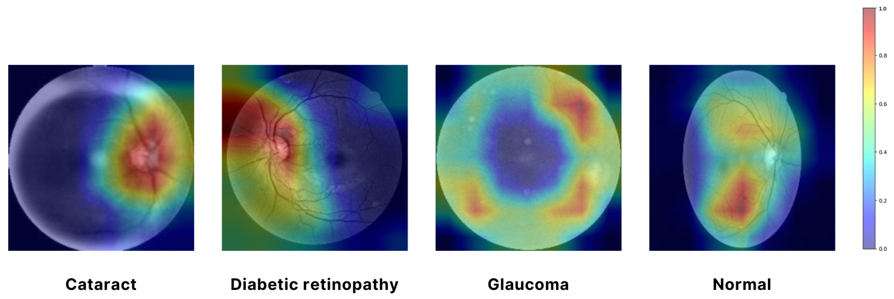
In Figure 7, a Grad-CAM (Gradient-weighted Class Activation Mapping) approach was employed to visualize the regions of input images that were most influential in the model’s decision-making process. Specifically, the EfficientNet architecture was used, and the Grad-CAM was generated by computing the gradient of the predicted class score with respect to the convolutional feature maps from the final convolutional layer. We utilized the EfficientNet architecture, which was selected as the final model for feature extraction due to its superior performance and efficiency. The resulting attention map highlights the spatial regions of the input image that contributed the most to the classification decision. By overlaying this attention map on the original image, we can intuitively observe which parts of the image the model focused on, thereby providing insight into the model’s interpretability. The use of Grad-CAM allowed for a visual explanation of the model’s predictions, ensuring that the areas with the highest activation were clearly identifiable and could be correlated with the salient features of the input images. In Figure 7, the red and yellow areas represent the most important regions of the image that the model relies on for making predictions. These areas have the highest influence on the model’s decision. Green areas are moderately important, contributing to the prediction but less so than the red and yellow regions. The blue areas are considered the least important, with minimal influence on the model’s output. This visualization aids in understanding the internal workings of the model. It confirms that it is focusing on the correct regions when making decisions, which is crucial for validating the reliability of the model in real-world applications [46].

5. Discussion

This work presented a systematic approach for automated eye disease classification from fundus images using ML and DL techniques. We make several notable contributions through our methodology and results. In this study, we utilized a variety of data sources to construct a sizable dataset of over 5000 fundus images across four classes—cataract, diabetic retinopathy, glaucoma, and normal. Many prior works have been limited by smaller datasets. By combining multiple open-access image repositories, we have been able to train more robust models. Then, we extracted deep features from the images using state-of-the-art CNN architectures like VGG, ResNet, and EfficientNet. We compared the performance of multiple networks to determine that EfficientNet provided the best feature representation for this application. Further dimensionality reduction through PCA retained the most useful features for classification. Systematically evaluating PCA over different feature counts provided insight into the optimal balance between accuracy and efficiency for us. After that, we trained a variety of ML models on the extracted and reduced features and analyzed their comparative performance. The best results were achieved using an SVM classifier, which attained 90% accuracy on test data after we tuned hyperparameters via Bayesian Optimization. Ensembling SVM with gradient boosting further improved efficiency for us. The 95.33 ± 0.60% overall accuracy surpassed most previous benchmarks on similar fundus image datasets.

The confusion matrices, ROC curves, learning plots, and K-fold cross-validation outcomes adequately validated the model’s generalizability. Comparisons to several transfer learning models also showcased the advantages of our proposed approach. While promising, some aspects could benefit from our further analysis. We could evaluate the model on additional unseen datasets to establish robustness. Testing model performance as dataset size or diversity varies would also be informative to us. Analyzing misclassifications may reveal areas for improvement in our model. Overall, this paper has made excellent progress towards accurate automated diagnosis from fundus images through the systematic machine-learning methodology that we have followed. The proposed BayeSVM500 model and analysis we have provided serve as a strong baseline for further research and applications.

6. Conclusions and Future Work

In this work, we developed an automated eye disease classification system using fundus images and ML techniques. We extracted deep features from images and reduced dimensions via PCA to identify optimal representations. We attained 95.33 ± 0.60% accuracy in detecting cataracts, diabetic retinopathy, glaucoma, and normal eyes using our BayeSVM500 model with a Bayesian SVM classifier. This surpassed previous benchmarks and transfer learning models evaluated. We provided comprehensive validation and explanations of model performance that could empower ophthalmic screening. While promising, evaluating model accuracy on larger unseen datasets, analyzing misclassification errors, enhancing efficiency, testing data dependencies, comparing advanced architectures, and employing generative techniques provided avenues for improvement in future work. With such enhancements to address robustness, efficiency, and resilience, our proposed methodology and model can serve as the core of automated systems assisting ophthalmologists in faster diagnoses to prevent vision impairment globally.