Article

MATLAB Application for Determination of 12 Combustion Products, Adiabatic Temperature and Laminar Burning Velocity: Development, Coding and Explanation

by
Roberto Franco Cisneros
* and
Freddy Jesus Rojas
*
Faculty of Mechanical Engineering, Pontificia Universidad Católica del Perú, Lima 15088, Peru
*
Authors to whom correspondence should be addressed.
Computation 2024, 12(9), 189; https://doi.org/10.3390/computation12090189
Submission received: 1 August 2024 / Revised: 6 September 2024 / Accepted: 9 September 2024 / Published: 16 September 2024

Abstract

:
The determination of the characteristics and main combustion properties of fuels is necessary for post-implementation in different applications. Among the most important combustion properties of a fuel are the combustion products, flame temperature and laminar burning velocity. Therefore, this paper describes the step-by-step development and coding of a MATLAB application that can determine 12 combustion products, flame temperature and laminar burning velocity in order to understand the logic of calculus procedure, so any user would be able to make improvements of new functionalities (add more fuels, add more combustion products, etc.). The numerical procedure and methods (Gaussian elimination, Taylor Series and Newton–Raphson) parallel with their implementation as code lines for the development of the application are carried out using flow charts. In addition, simulations in Ansys Chemkin were performed and included in the application as part of the results comparison. It was found that: (1) The MATLAB Application codification and development were successfully explained in detail, (2) the functions and execution sequence are described by using flow charts and code extract, (3) the application is available to everyone for modifications, (4) the application can only be used for hydrocarbons fuels, (5) the application execution time registered was less than 8 s.

1. Introduction

The simulation of combustion processes remains a key component in the development and design of new engines, power sources, and machinery. Among the different studies that facilitate the acquisition of new results, there are numerical procedures, experimental tests, and software simulations. Software tools such as Ansys Chemkin, Cantera, and other applications are necessary for obtaining an initial understanding of the combustion process as they provide critical data on new systems under development.
Within the previous research conducted by various authors, different programs and codes have been used for many applications. In 1989, Zhu and Egolfopoulos made a numerical simulation of one-dimensional flame propagation by using a flame code developed by Kee and coworkers that has in its program multicomponent diffusion relations, mass conservation equation and a C1 kinetic mechanism developed by the same author [1]. Starting in the 2000s, Tsotsis and Egolfopoulos used the PREMIX code developed in FORTRAN for determining the mole fractions of the products, and the laminar burning velocities of different methane–CO2 mixtures [2]. In 2012, Erjiang et al. studied the effect of composition on laminar burning velocities of H2/CO/N2/CO2/air mixtures using experimental and numerical studies. In the latest one, they simulated using PREMIX code with CHEMKIN II a freely propagating adiabatic premixed planar flame [3]. In this study, the Li Mechanism, Davis Mechanism, USCII Mechanism, GRI-MECH 3.0 Mechanism and Sun Mechanism kinetics were used [3]. Seven years later, Longkai et al. did a numerical analysis of the effect of CO2 on combustion characteristics of laminar premixed methane/air flames. Similar to previous works, they used the PREMIX code for the calculation of the one-dimensional laminar premixed combustion characteristics of (CH4 + CO2)/air mixtures with different CO2 contents and equivalent ratios [4]. Later, in 2020, Xie et al. employed the Premixed Laminar Flame-speed Calculation model to calculate the one-dimensional free propagation flame with the PREMIX code of Chemkin package for a numerical analysis on the effects of CO2 dilution on the laminar burning velocity of premixed methane/air flame with elevated initial temperature and pressure [5]. All equations of PREMIX code use can be found in the Chemkin-Pro 19.0 theory manual [6].
Programs and programming languages such as MATLAB, PYTHON or FORTRAN are preferred by the scientific community for a wide range of applications as they have enough features for the analysis process. In the MATLAB App Designer, it is possible to create various apps to observe and analyze the results of different studies in a more intuitive manner. For this study, the main contribution is the detailed description and explanation of the development of the MATLAB Application. Considering the main reference to the FORTRAN code developed by Olikara and Borman [7], which already includes the numerical methodology for calculating flame temperature and combustion products, a new package of codes was created in MATLAB. This new one compared with the Olikara and Borman FORTRAN has the novelty of including the determination of the laminar burning velocity. Finally, a MATLAB Application was developed including the new package of codes and all the features detailed in the present work. Code lines and flow charts are presented to help readers understand the programming logic for future improvements of new tools, new fuels or new combustion products. This work is a sequence of the published article “Determination of 12 Combustion Products, Flame Temperature and Laminar Burning Velocity of Saudi LPG Using Numerical Methods Coded in a MATLAB Application” that previously has presented the validation of the app [8]. The methodology of the project is explained, and the results obtained are compared with different experimental and numerical articles for some fuels (methane, propane and natural gas).

2. Materials and Methods

The numerical method was originally developed in FORTRAN in 1975 by Olikara and Borman in their paper titled “A Computer Program for Calculating Properties of Equilibrium Combustion Products with Some Applications to I. C. Engines” [7]; and modified to include the determination of the laminar burning velocity by using MATLAB R2021b for the codes package and the MATLAB App Designer for the development of the application. The simulation results included in the application were carried out in Ansys Chemkin 2022 R2. Figure 1 presents the methodology diagram for the PI075 Project.
A computer with an AMD Ryzen 7 5700G with Radeon Graphics 3.80 GHz processor with 32 GB RAM and Windows 11 Enterprise was used for this purpose.

3. Development of the MATLAB Application

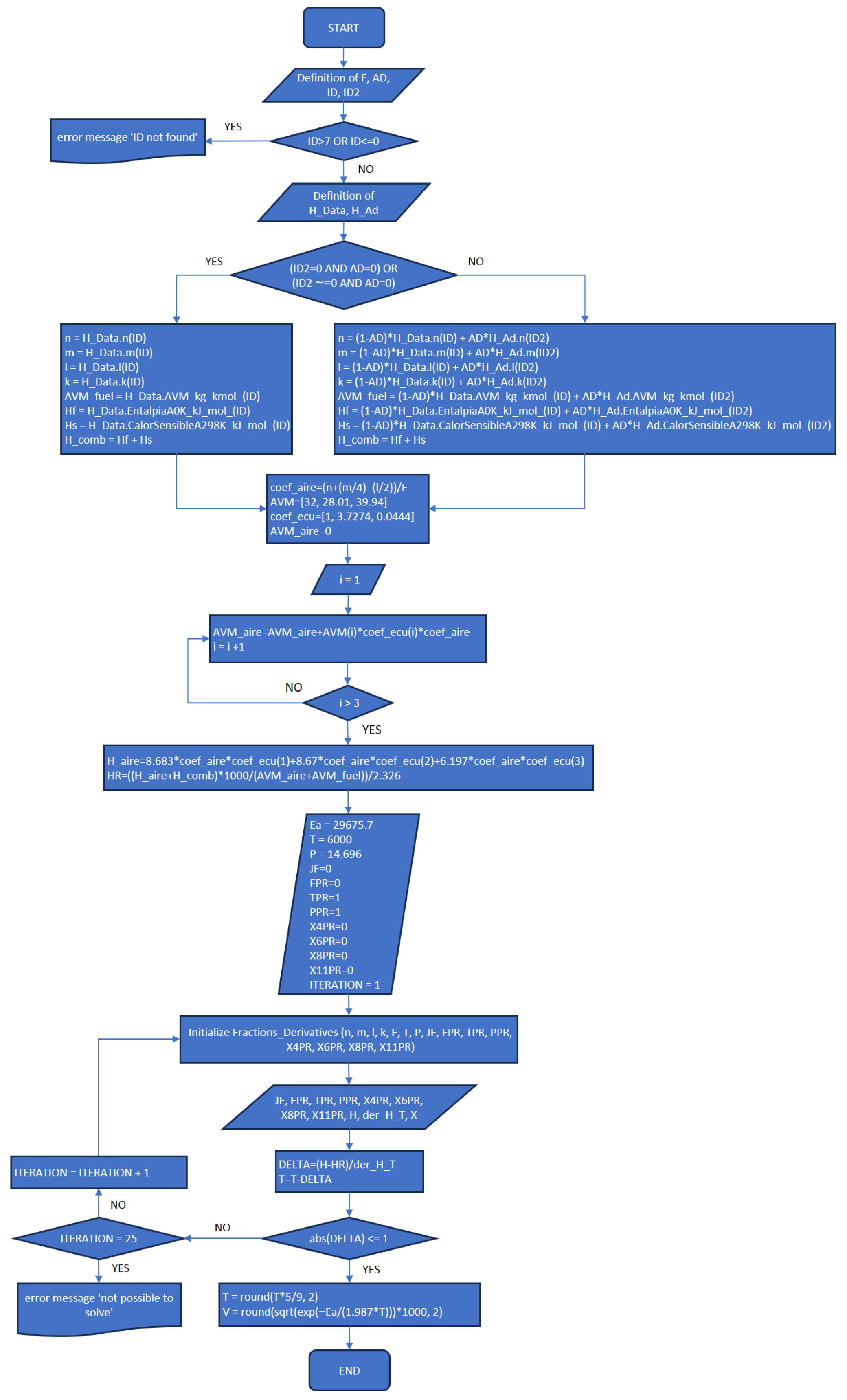
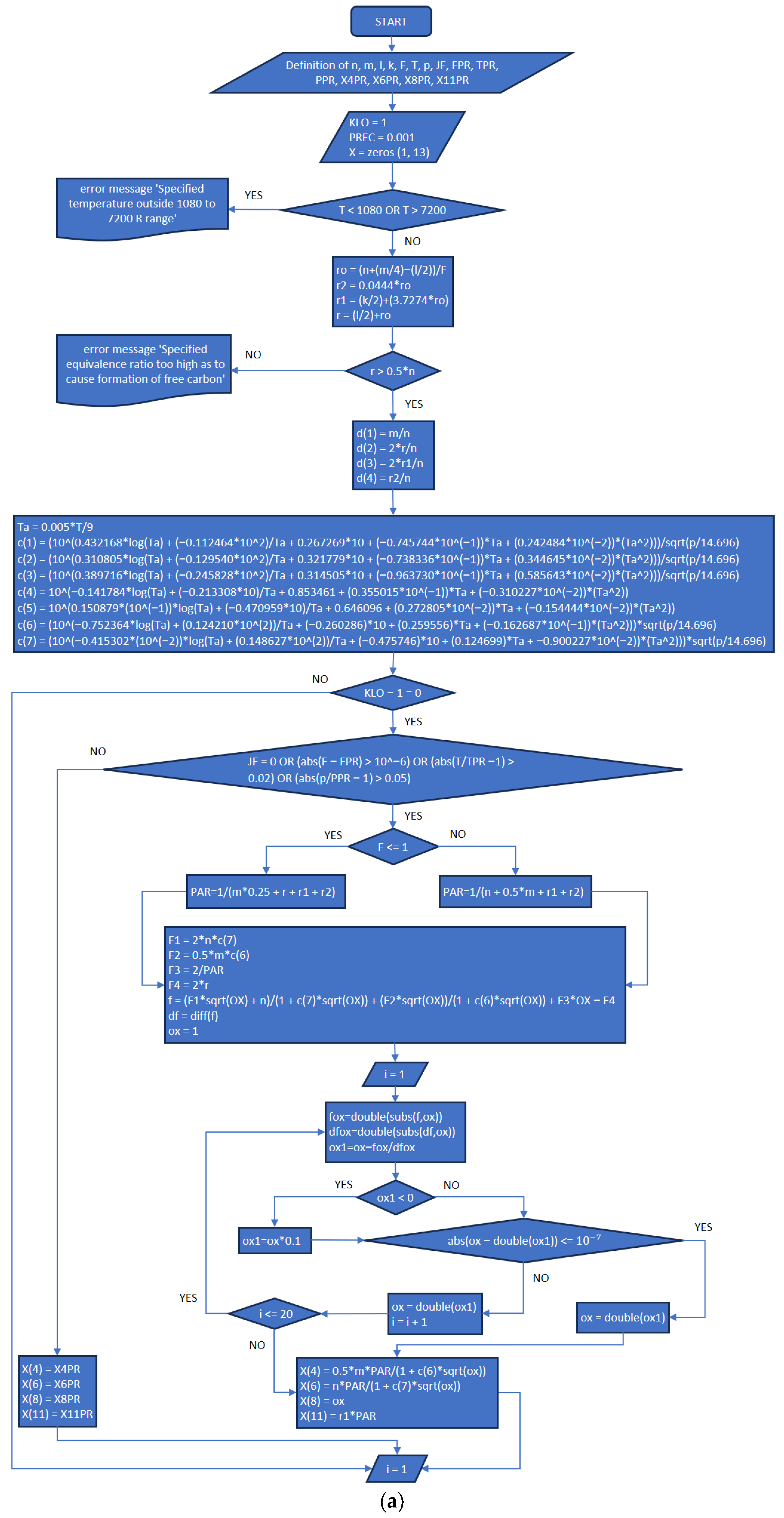
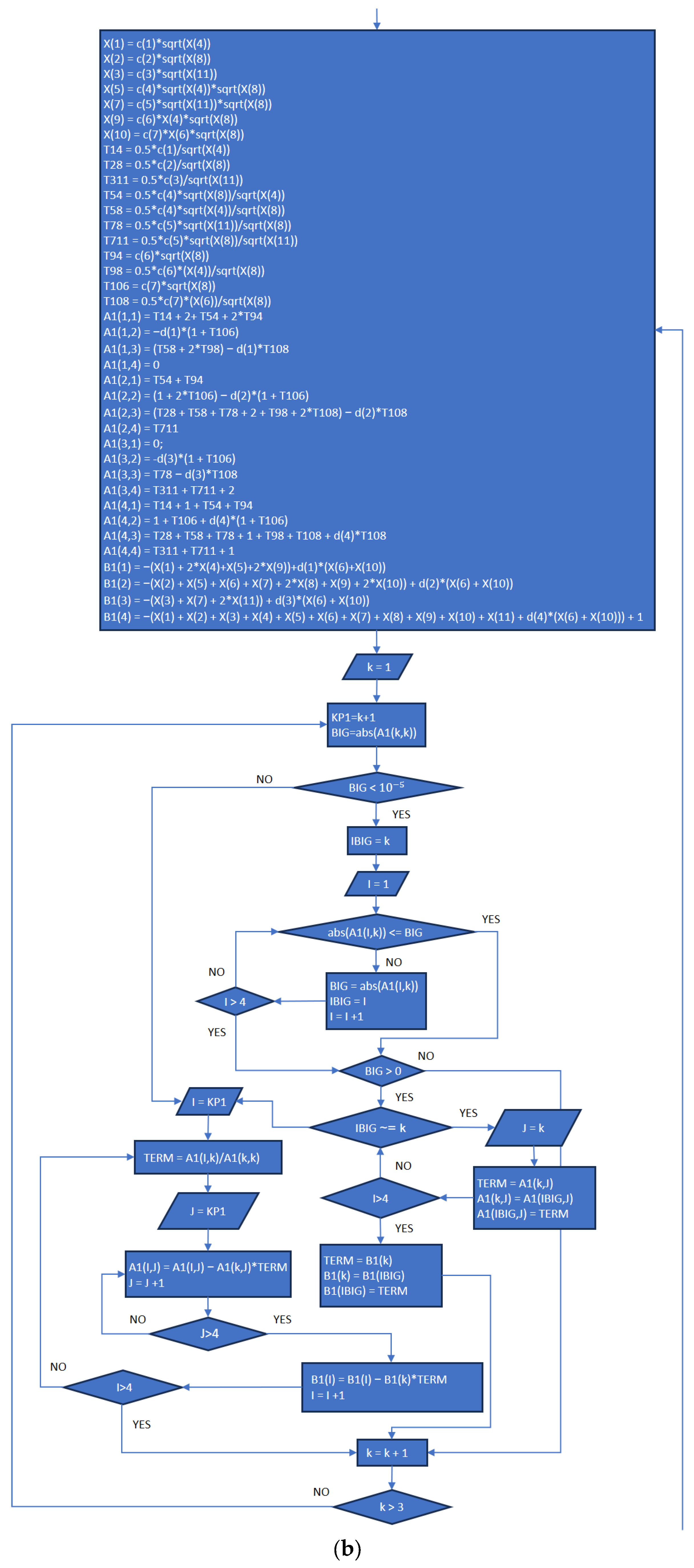
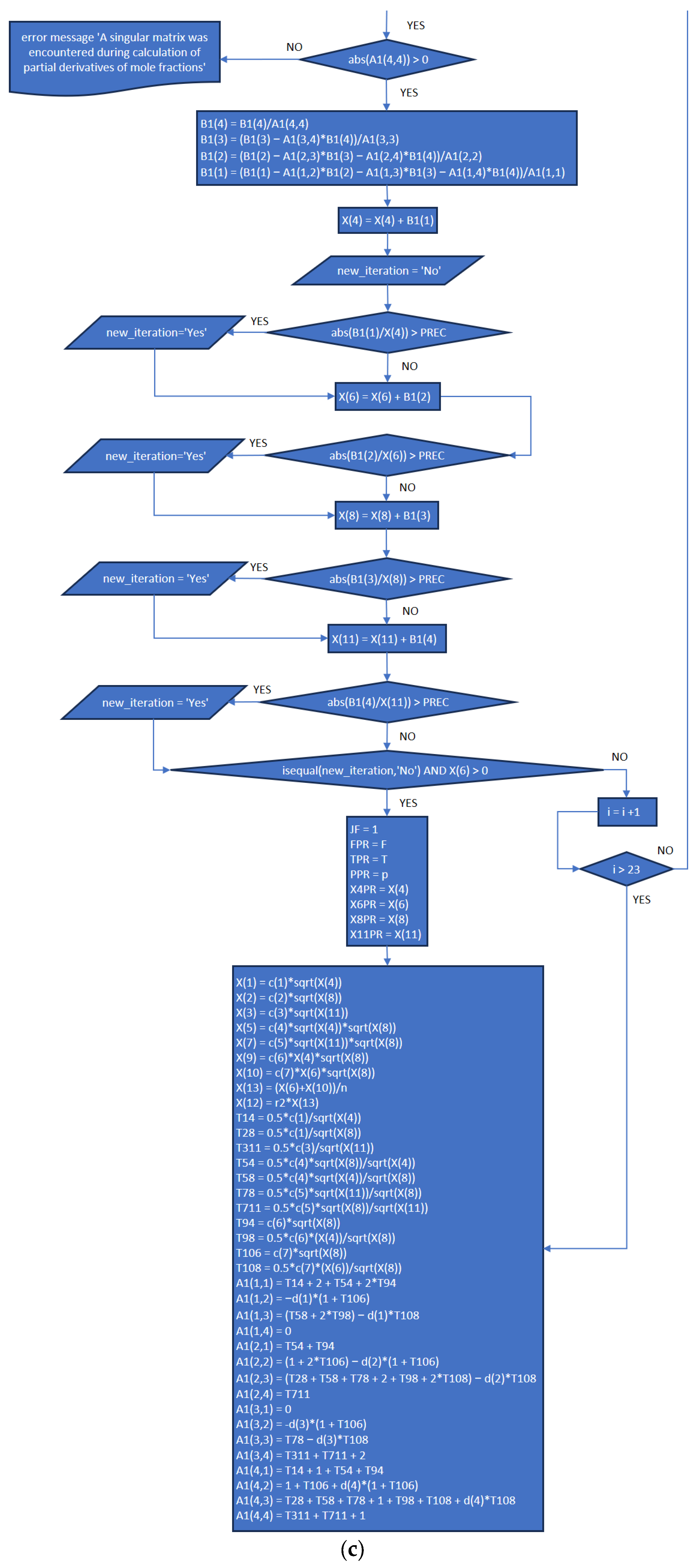
The application designed in MATLAB is divided into three main parts; for each one, a flowchart of how the code works was constructed which can be found in Appendix A. The first one (Figure A1) receives all the necessary inputs to start the iteration process until the adiabatic temperature is found. Secondly, in Figure A2, all the numerical matrices and derivative-necessary operations are performed, so the combustion products and other important values are obtained. Finally, Figure A3 explains how the initialization of the process of the application works. Theorical energy equations and statements have already been explained and presented in the previously published article referenced as [6].

3.1. Part One: Develop of the “New_code” File

This first part (Code S1) starts with the necessary inputs for the iteration process: the equivalence ratio (F), the fraction of the diluent (AD, if applicable), the ID of the fuel (ID assigned in File S1 called “REACTANTS ENTHALPY” with the properties of the fuel) and the ID of the diluent (ID2 assigned in File S2 called “DILUENT ENTHALPY” with the properties of the diluent if applies). The first step is a verification of the existence of the introduced fuel ID in the database File S1 as shown in Figure 2. Then, it is possible to define the variables H_Data (Enthalpies values) and H_Ad (Enthalpies diluents values), as these variables will store all the data related to the reactant and the diluent (if applicable), respectively.
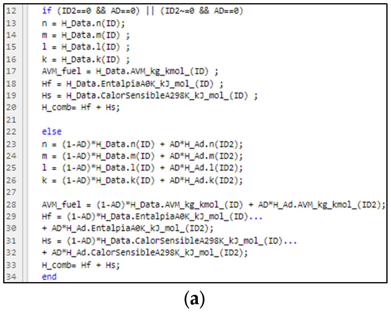
After the verification, it is possible to calculate the fuel enthalpy with the ratio of equivalence, the specified fuel and the fraction of diluent (if applicable) by using the variables H_Data and H_Ad that were defined previously, as shown in Figure 3.
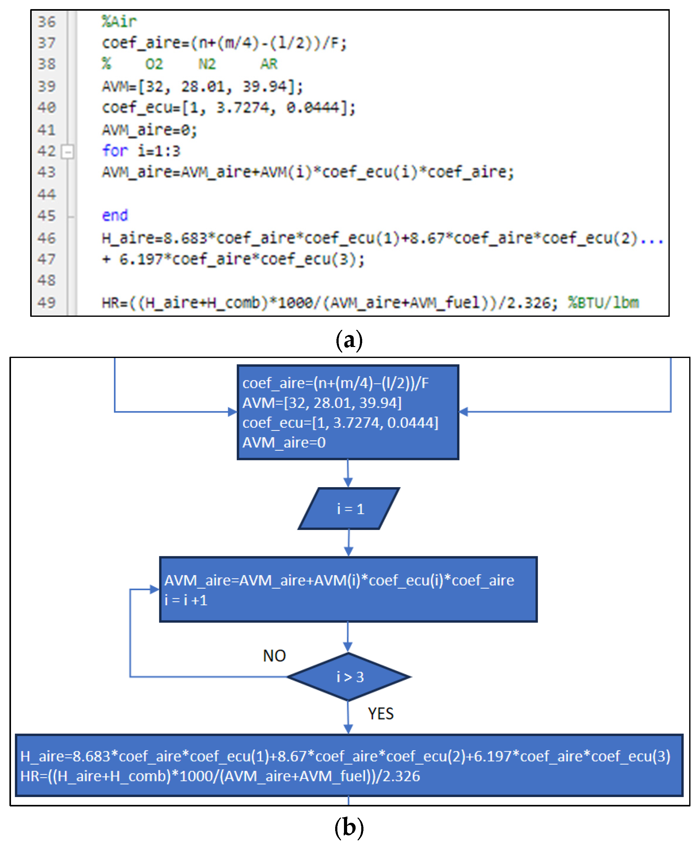
The next step is to calculate the air enthalpy using the ratio of equivalence, the coefficients related to the fuel (n, m, l, k) and the AVM which is defined as a matrix. The whole reactant enthalpy (air plus fuel) is calculated as shown in Figure 4.
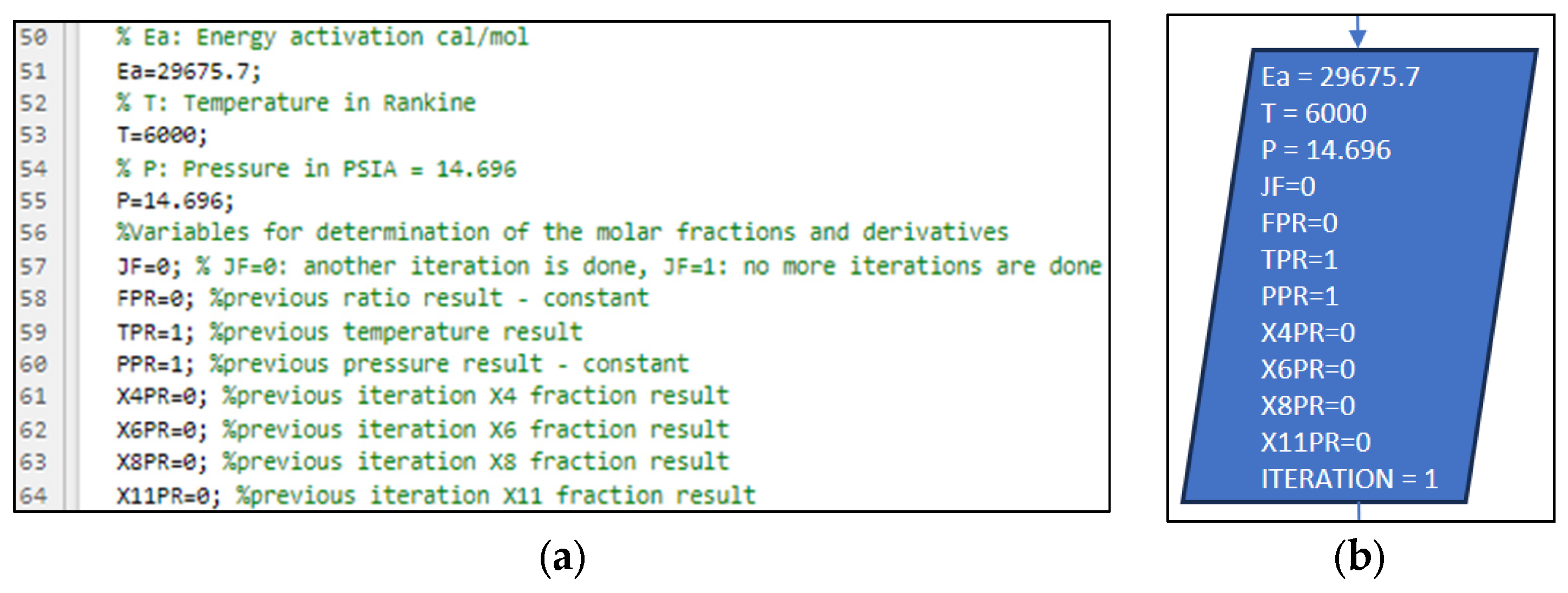
Following the previous step, it is necessary to set the Activation energy (Ea), which is defined as equal to 29,875.7 cal/mol, the first estimated temperature (T) 6000 R, the work pressure (P) 1 atm or 14.696 psi and the variables necessary for the iteration process required to determine the 12 combustion products, as shown in Figure 5.
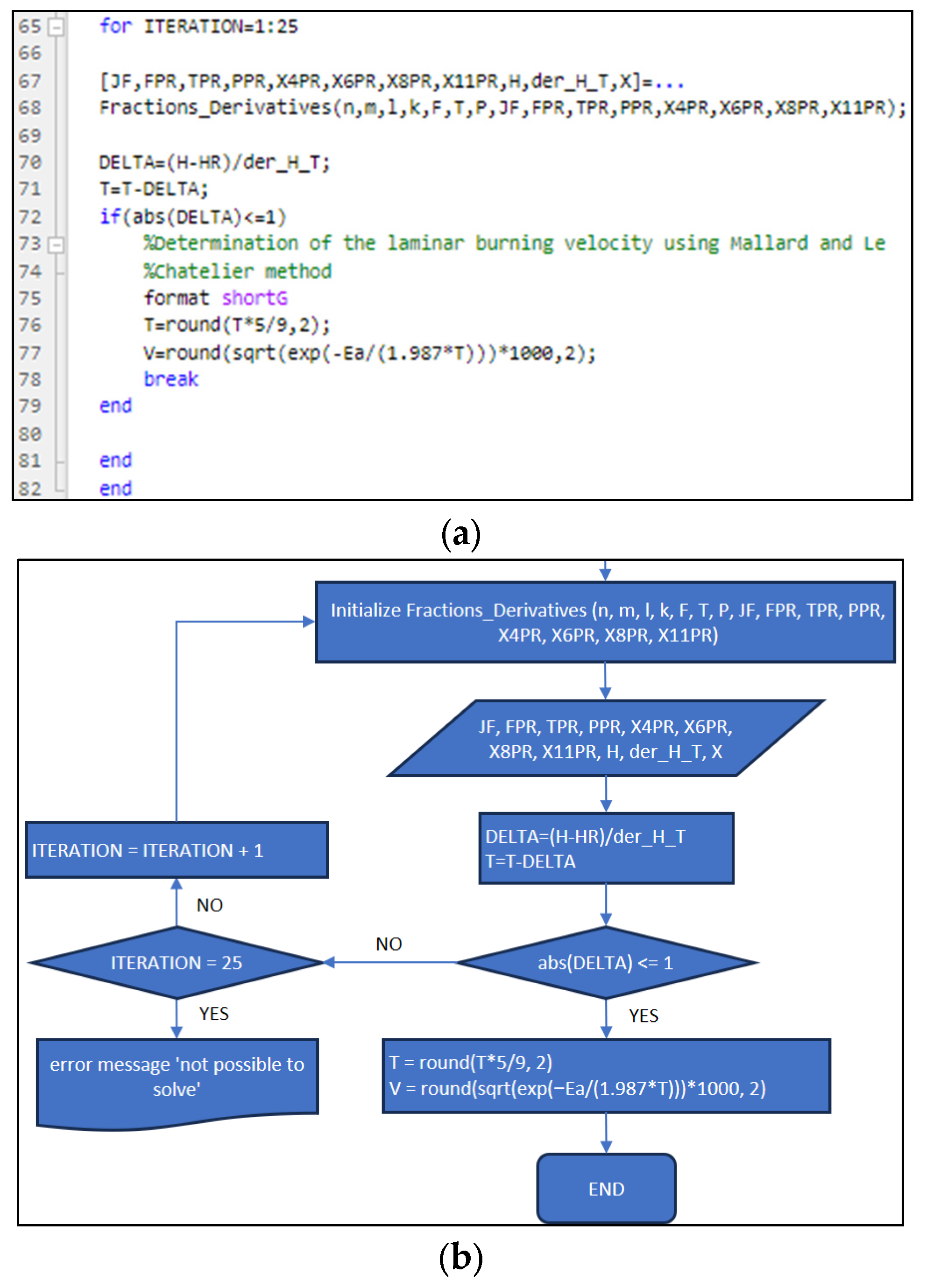
These variables and all the inputs that are defined in Figure 5 are introduced in the function Fractions_Derivatives where the iteration process begins. DELTA is calculated using the reactants (HR) and Products Enthalpy (H) difference, divided by the derivative of enthalpy respect temperature (der_H_T). The loop finish when DELTA is less equal to 1 so the flame temperature (T) and laminar burning velocity (V) can be calculated using the Mallard and Le Chateller method as shown in Figure 6.

3.2. Part Two: Develop of the “Fractions_Derivatives” File

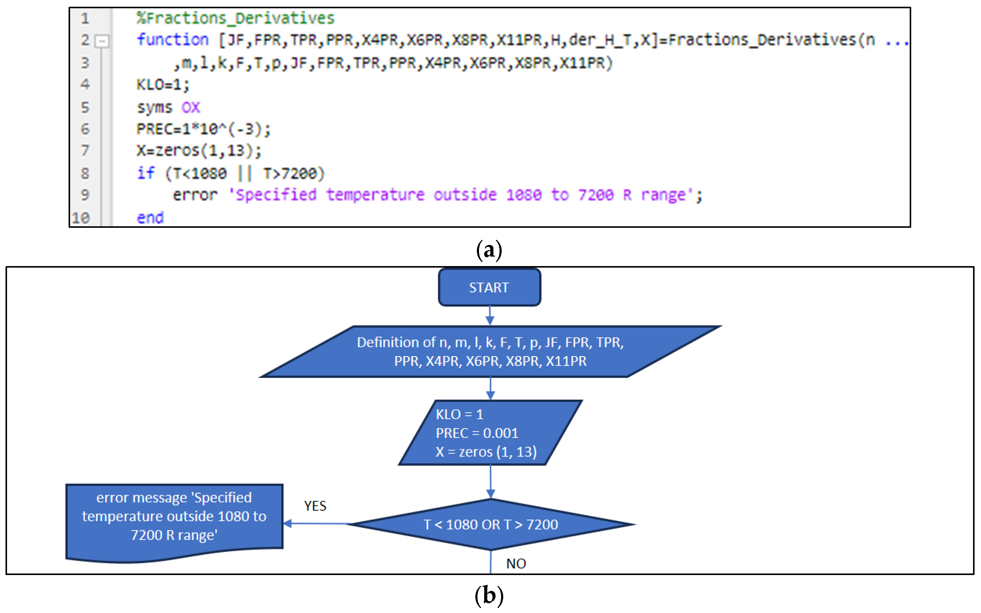
For part two (Code S2), the first action performed by the program is to define the size of the matrix for combustion products (X), the precision for the calculations and verify if the first estimated temperature defined in the first part (6000 R) or the calculated for a specific iteration is between the range of 1080–7200 R as shown in Figure 7.
The next step in the process is the definition and determination of the constants related to the combustion reaction balance. In addition, verification of the equivalent ratio is performed to ensure that it is not too high which can cause the formation of free carbon because this would not let the application solve the equation system, as shown in Figure 8.
A temperature Ta is defined as an input in the equilibrium constants at constant pressure (Kp) for each reaction which is shown in Figure 9.
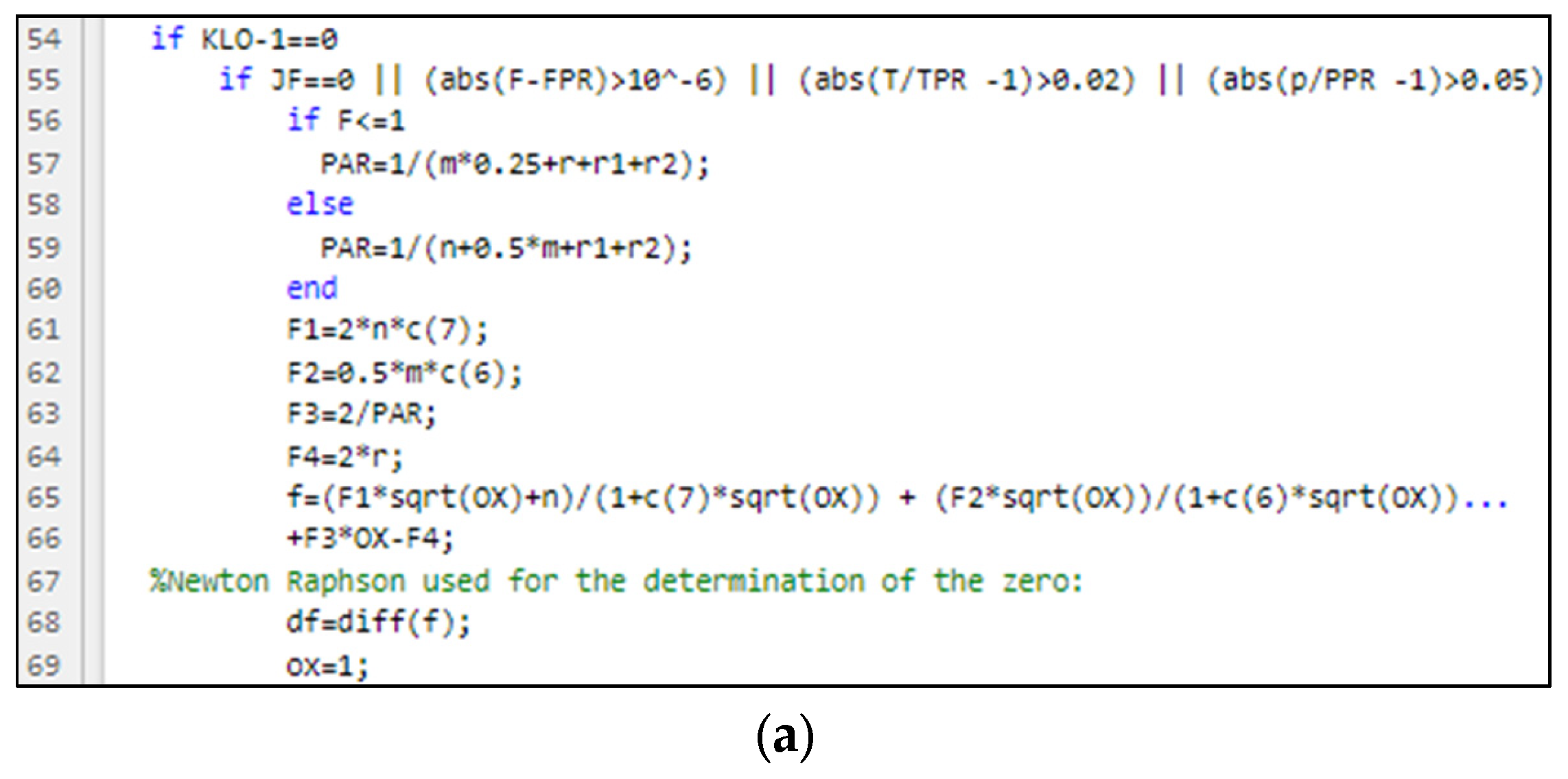
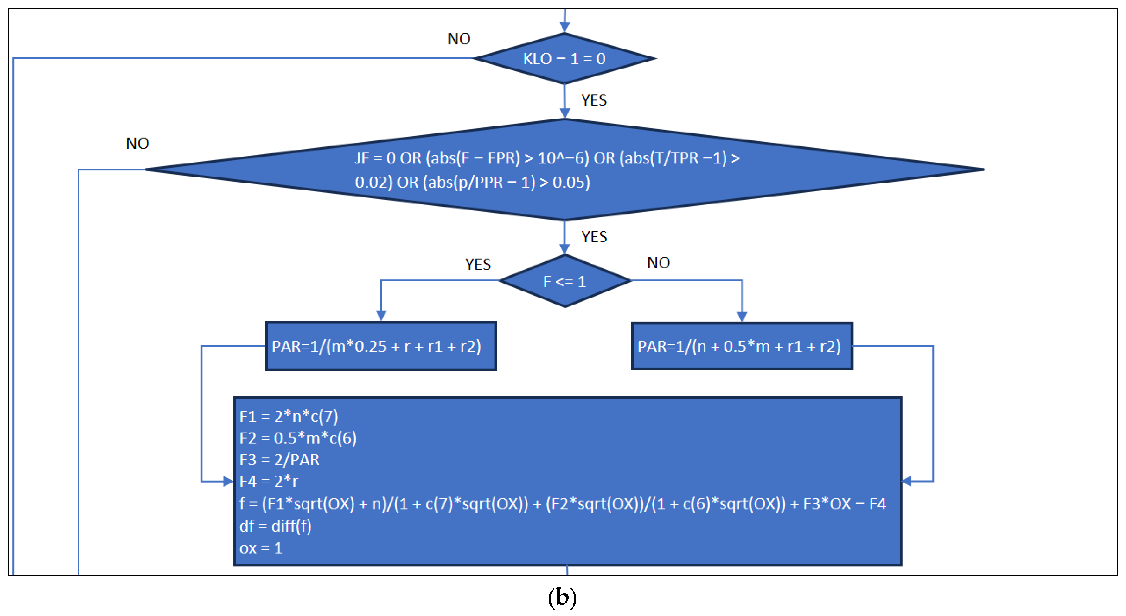
After the Kp constants are defined, depending on the ratio of equivalence that is going to be used, an “if” condition is stated for ratios less equal 1 and for greater than 1. With the “if” condition a first estimated value of ‘PAR’ (that represents x13) is calculated with variables ‘F1’, ‘F2’, ‘F3’, ‘F4’ and ‘f’ (general linear function). Later, the first differential equation of ‘f’ is calculated (‘df’) and ox (first estimate value of x8) is defined in order to start the Newton–Raphson iteration process as shown in Figure 10.
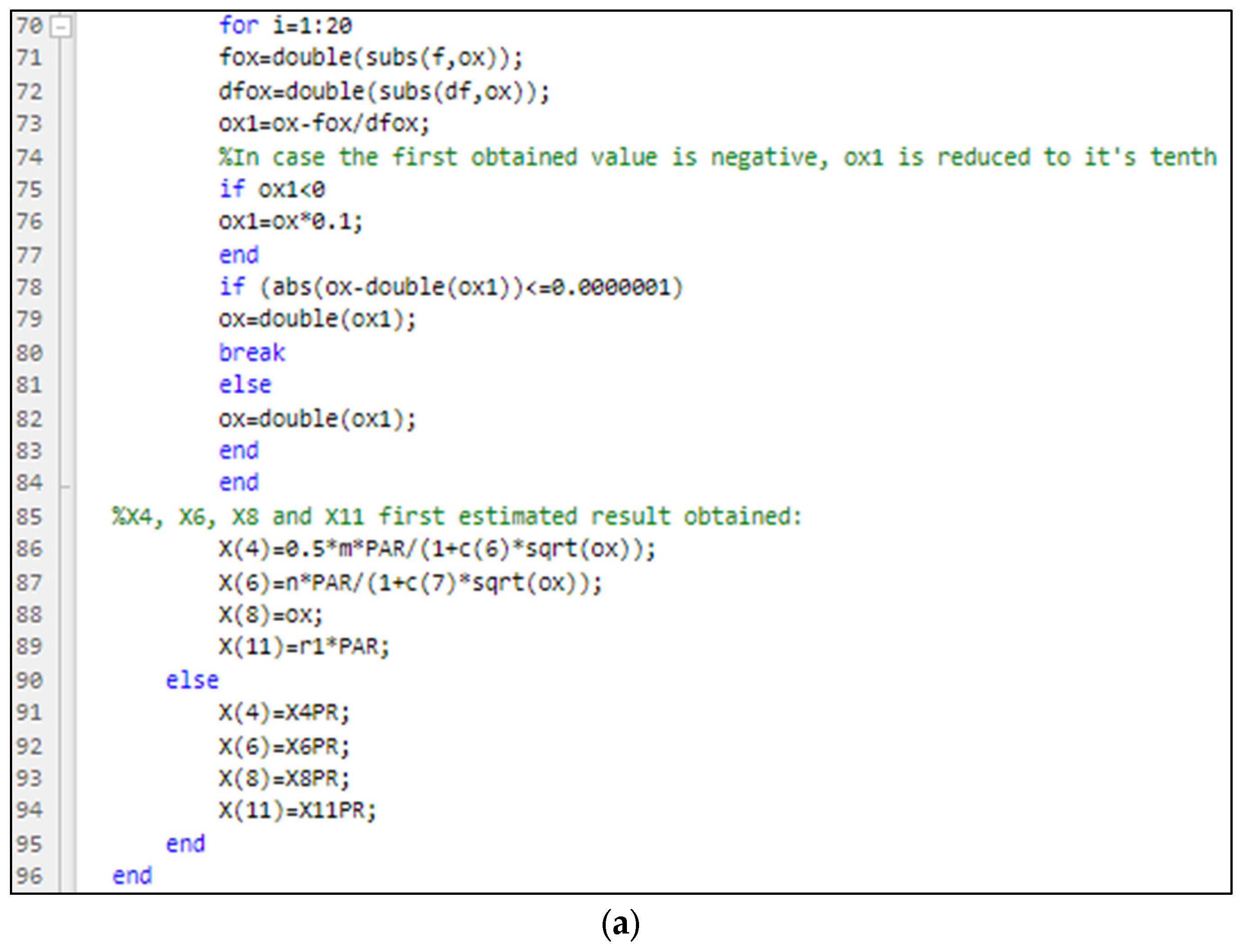
With ‘df’ it is possible to determine the first estimated values of x4, x6, x8, x11. The Newton–Raphson method is applied in order to find the zero of equation ‘f’. Two variables ‘fox’ and ‘dfox’ are defined in order to store the value of ‘ox’ replaced in ‘f’ and in ‘df’, respectively. The Newton–Raphson process is set to take 20 iterations maximum as a limit as during simulations for all the pre-set fuels, and the iteration process mostly ends at the 8th iteration. This number of iterations also helps in the case of new fuels that might be added and could require more iteration time. After the iteration process successfully fulfils the tolerance (less equal 0.0000001), the values of x4, x6, x8, and x11 are calculated using the previously defined equations as shown in Figure 11.
After a first estimate of the values x4, x6, x8, x11, it is possible to define the other products using these values. In addition, the values of the derivatives for each molar product respect x4, x6, x8, x11 and the four functions (Bj) are also defined as shown in Figure 12 in order to form a matrix equation system.
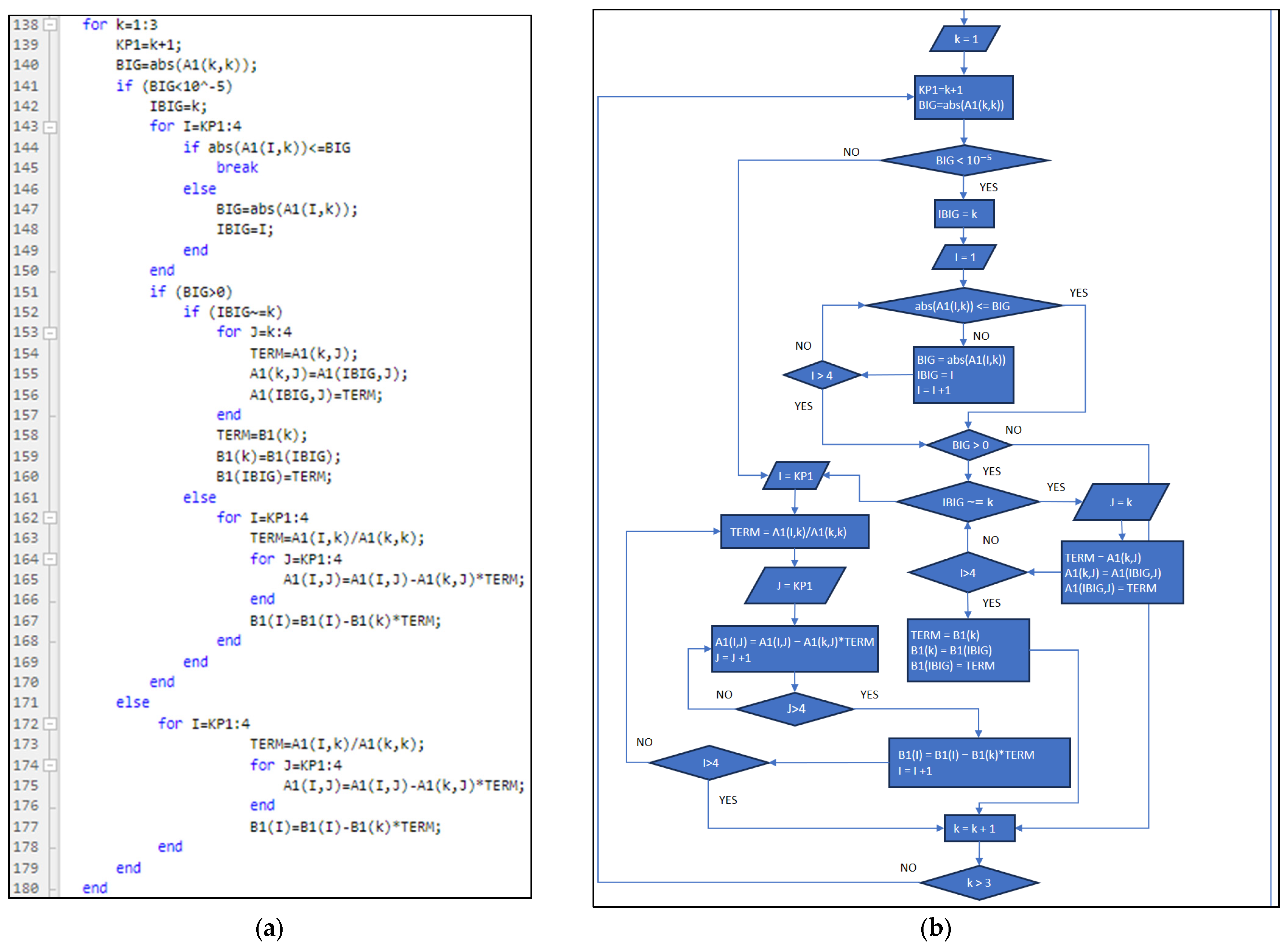
Once the matrix system is defined, the Gaussian elimination method is applied using row interchange only if the pivot point is smaller than 10−5. This, in the code, is a for loop and has some restrictions in order to obtain the modified matrix. All of this process is shown in Figure 13.
In the case that the existence of a singular matrix occurs, an error message will be displayed as shown in Figure 14.
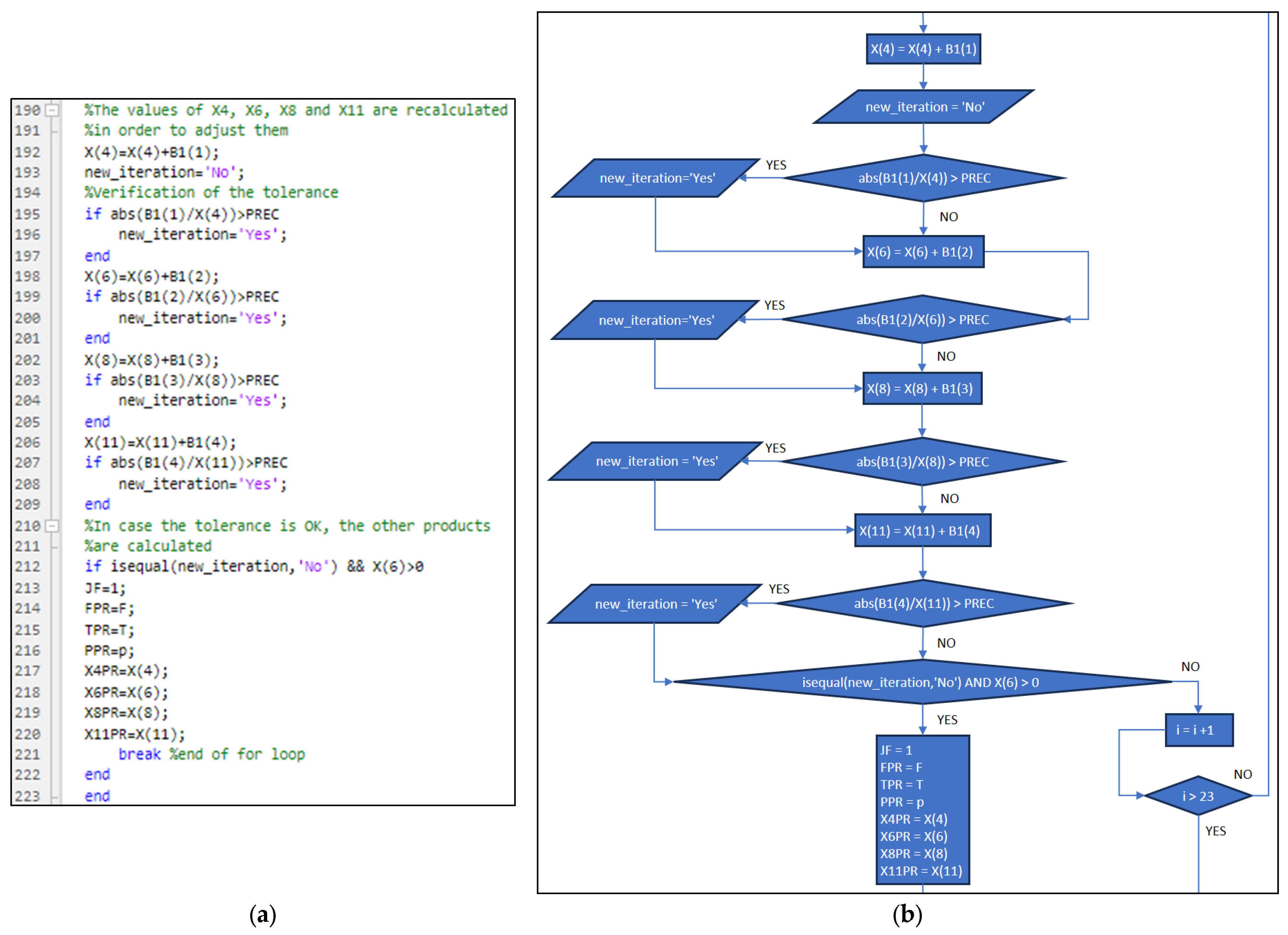
After doing the verification, in case there is no error, the values of x4, x6, x8, and x11 are calculated one more time in order to adjust them and the tolerance is verified. Moreover, the value of the variable “new_iteration” is “No” until the end, which will be the end of the iteration process in the matrix, and the other products are calculated as shown in Figure 15. If the opposite happens, another iteration is carried out.
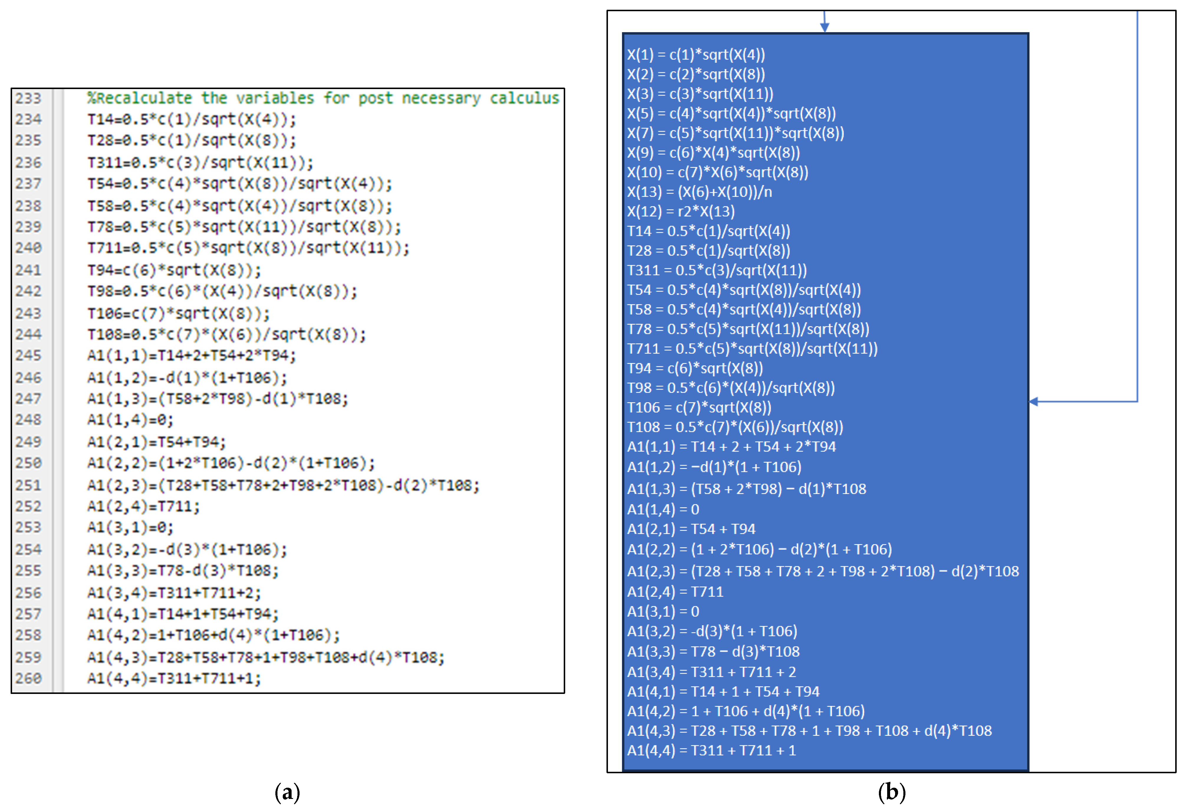
After finding the molar products, it is necessary to recalculate the previous variables (derivatives of molar products and functions F1, F2, F3 and F4) in order to have them available for post-calculus as shown in Figure 16.
Moreover, the properties of products (molar mass—SM, enthalpy—HT, specific heat capacity—CT) are added into the program by reading File S4 which contains them, as shown in Figure 17. The properties will be used for the final determination of the specific enthalpy of the whole products.
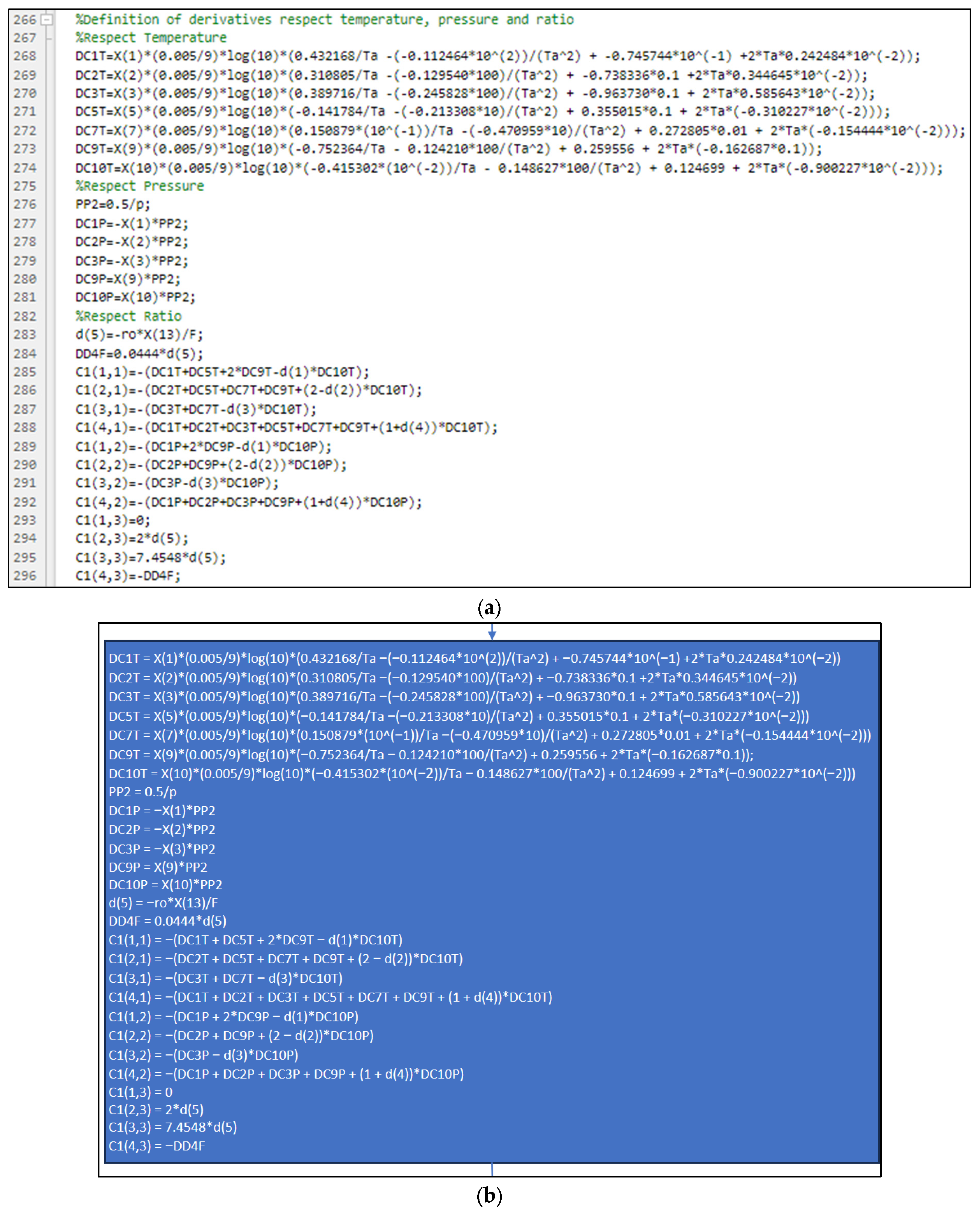
The next step is to define the derivative respect temperature (DCT), pressure (DCP) and ratio (DD4F), as shown in Figure 18, in order to determine the derivative of enthalpy respect temperature (der_H_T), which depends on the value of the derivative of mole fraction respect temperature and the derivative of molar mass respect temperature.
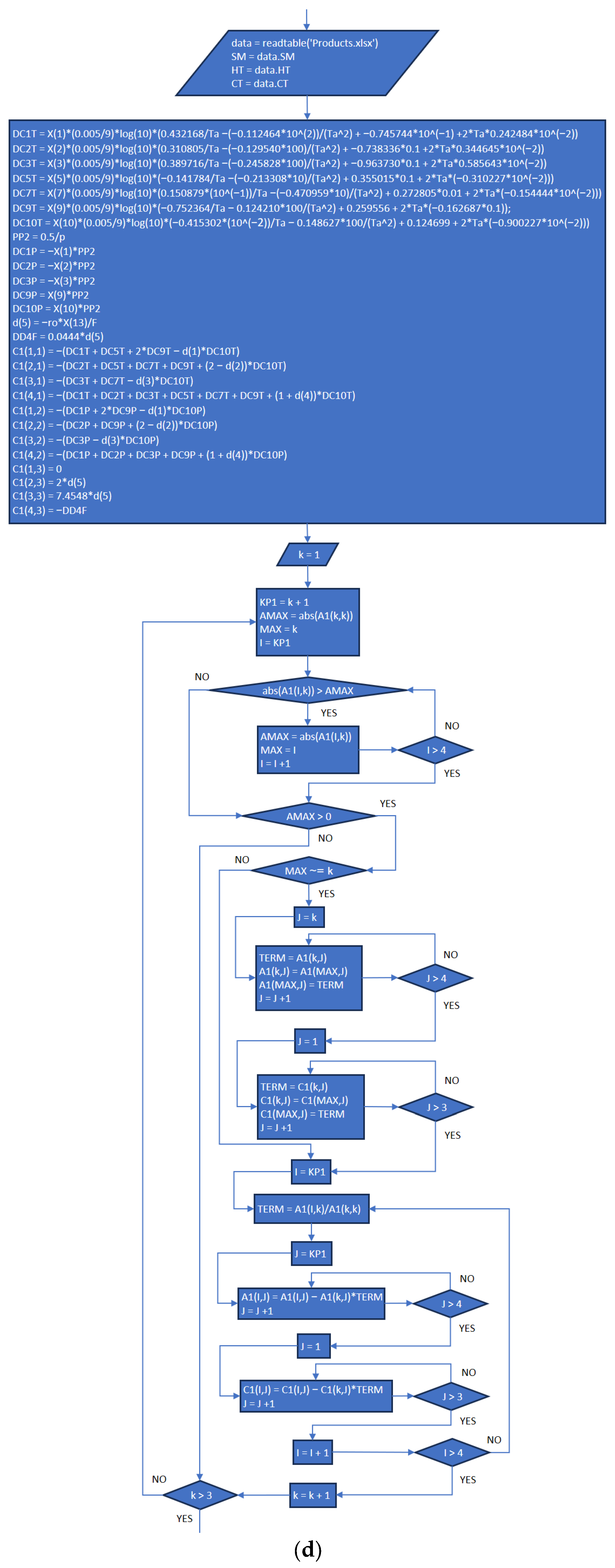
After defining the derivative respect temperature, pressure and ratio, and setting the new equation systems (C1 equations matrix), the Gaussian elimination using maximum pivot strategy is used for the solving the matrix equation system as shown in Figure 19.
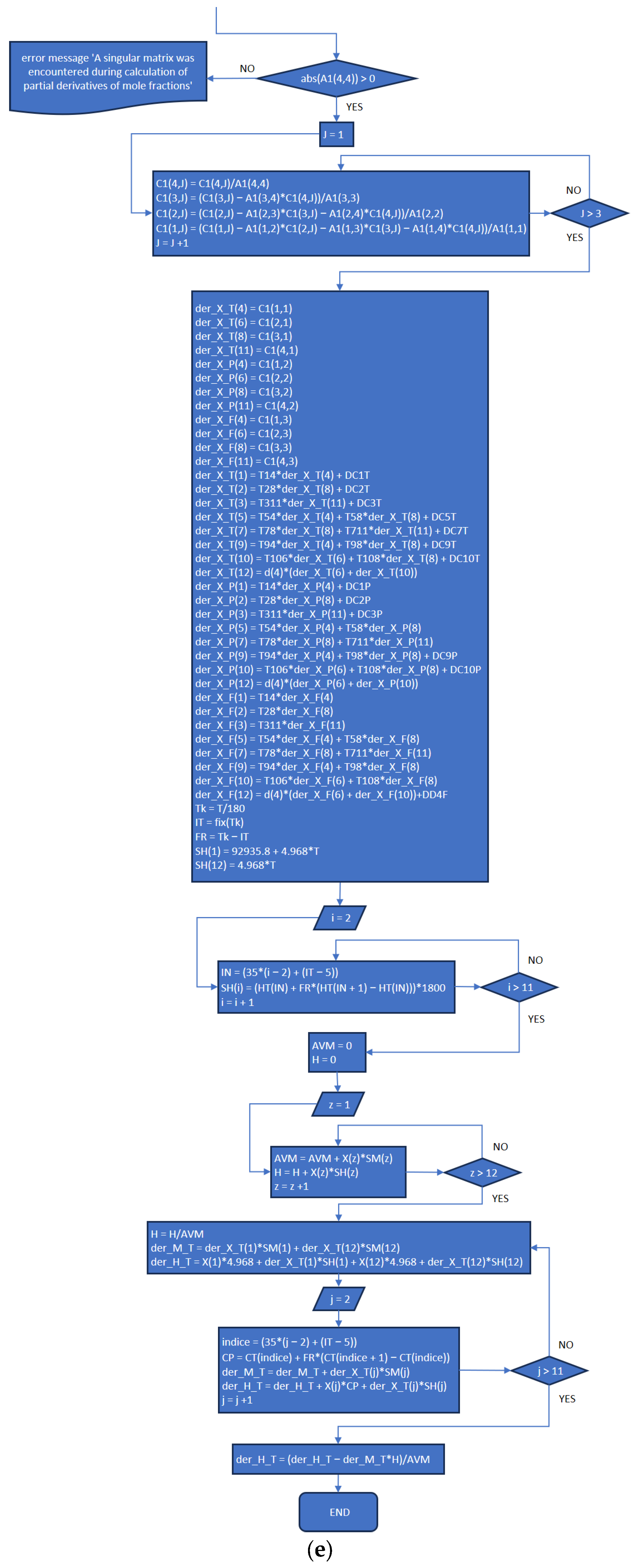
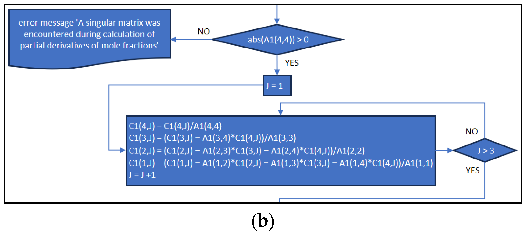
After completing the maximum numbers of iterations, a verification of the value of A1(4,4) is performed in order to validate if any singular matrix was found. In the case that it passes the validation, each element of the matrix C1 is calculated, because they contain the derivatives of each property. As the matrix has three columns and four rows, an iteration is necessary for each column in order to calculate each element as shown in Figure 20. In the opposite case, an error message is displayed.
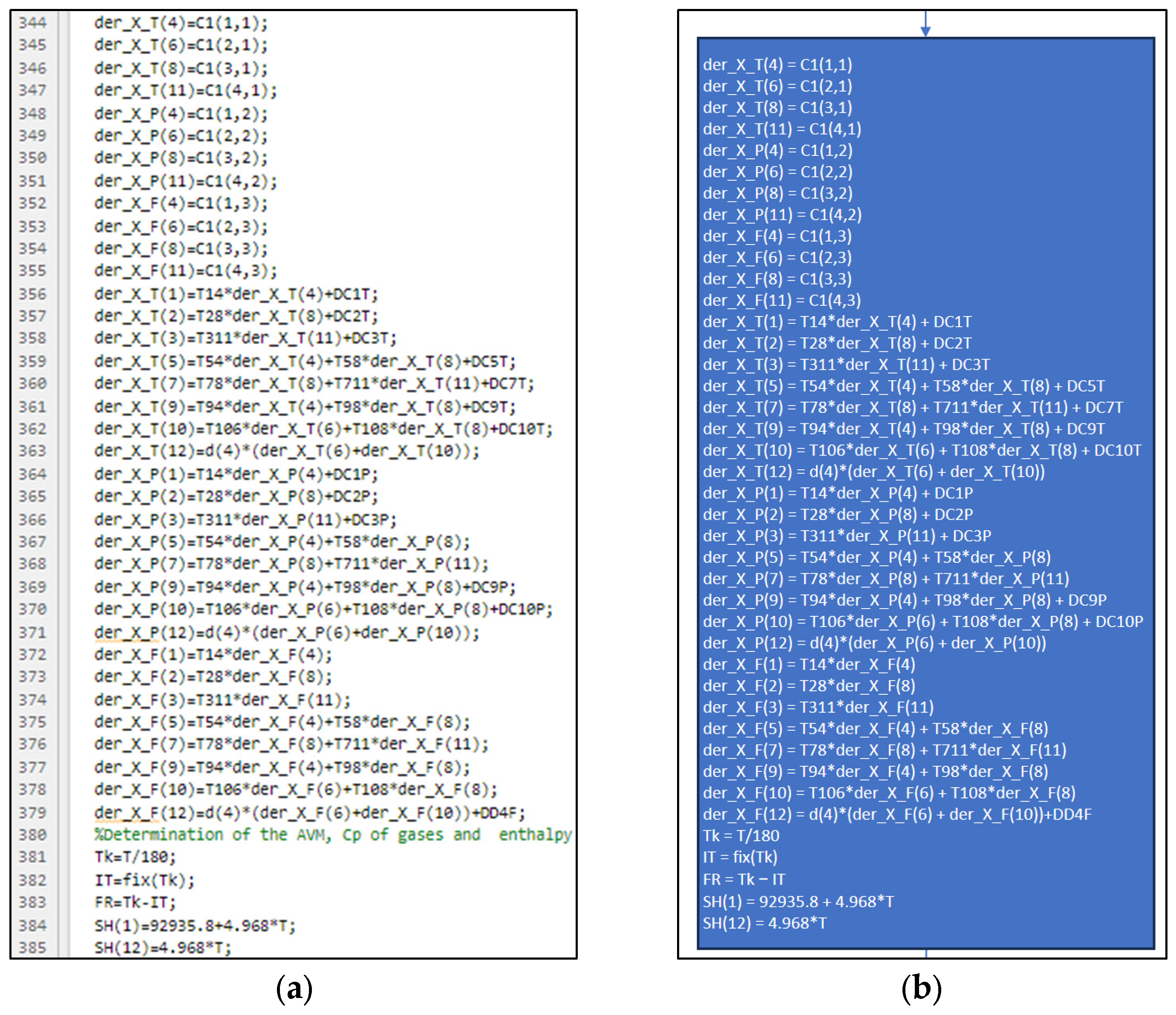
Then, the partial derivatives with respect temperature, pressure and ratio are calculated using each element of the C1 solved matrix, and ‘Tk’, ‘IT’, ‘FR’, ‘SH (1)’, ‘SH (12)’ are calculated and defined for the determination of product enthalpy (H) and average molar mass (AVM) as shown in Figure 21.
The enthalpy of each product is calculated and stored in a single row matrix (SH) as shown in Figure 22.
By using the enthalpy of each product SH, the average molar mass (AVM) and product enthalpy (HR) are calculated as shown in Figure 23.
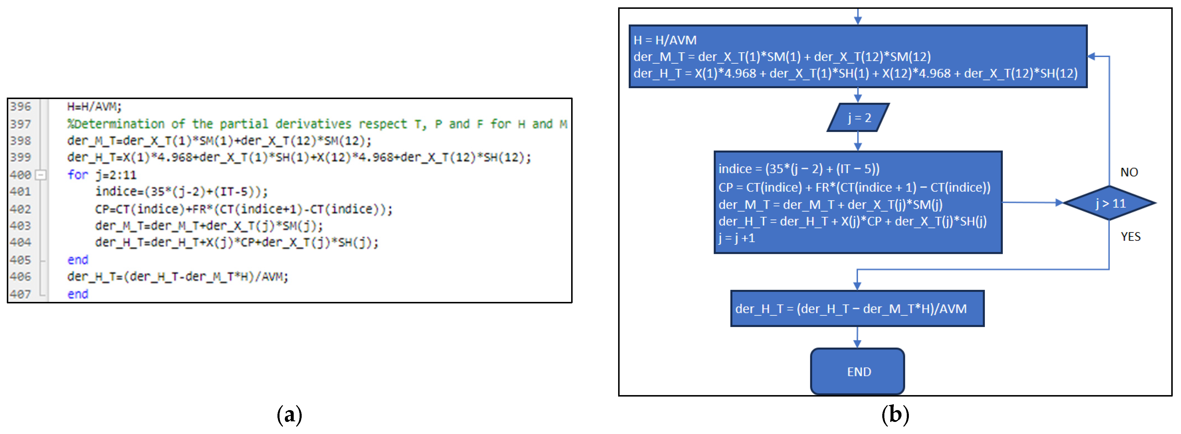
The specific product enthalpy is calculated dividing the product enthalpy by the average molar mass, and the partial derivatives with respect temperature are calculated for enthalpy and molar mass just for the first and last products (1 and 12). Iterating between 2 and 11 values, the CP (constant pressure heat) is calculated, and it is possible to determine the final value of the partial derivative of enthalpy with respect temperature that is needed for the DELTA determination in New_code.m as shown in Figure 24.

3.3. Part Three: Develop of the MATLAB Application File

In this part, the code and flowchart when the application is initialized is explained. In addition, the tools of the MATLAB Application are explained along with how they work through the programming code. When the application is started, the properties that variables that can be used in any function defined in the application are specified as shown in Figure 25.
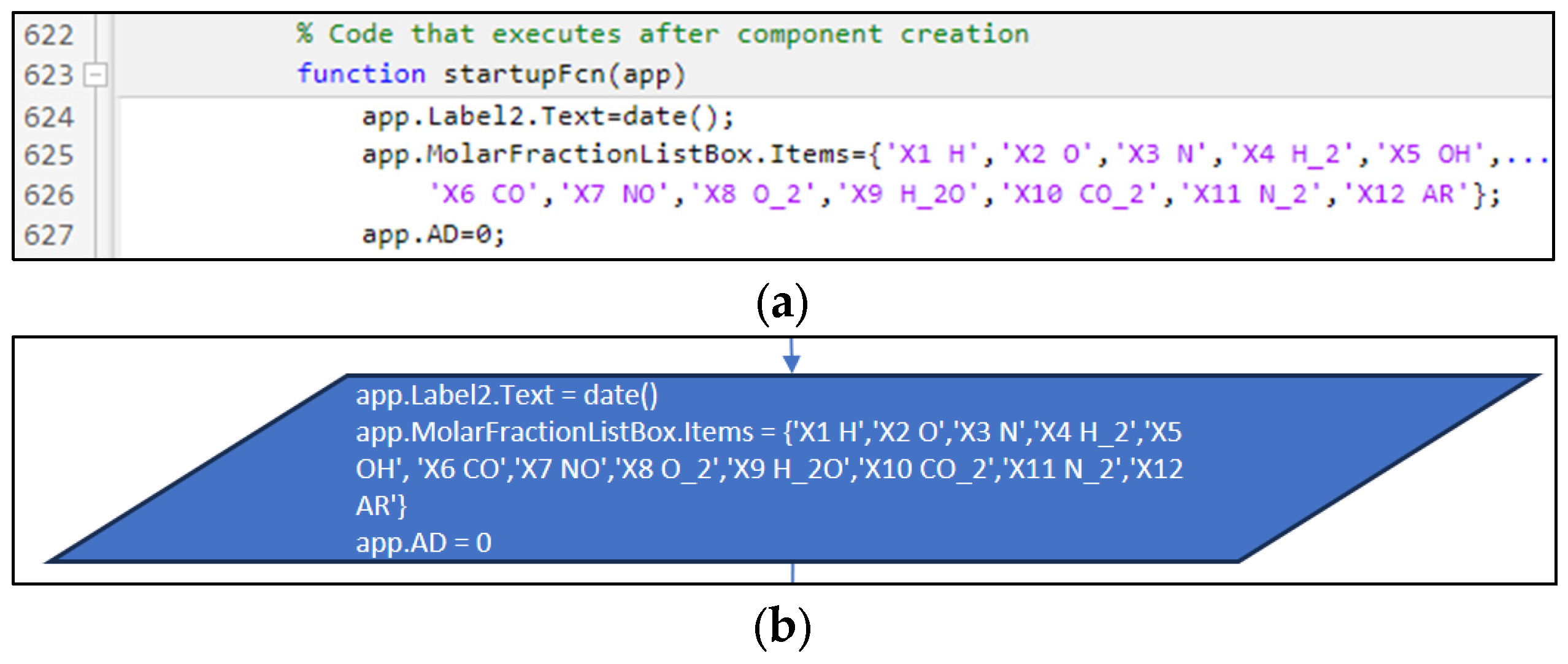
Then, when the application is started, ‘Label2’ is defined to show the current date and the molar fraction list item is set. The default value assigned to the variable corresponding to the diluent app.AD is 0 as shown in Figure 26.
The reactant enthalpy excel archive is also used during the determination of the products, and temperature and burning velocity are used for defining the list of fuels that will be considered in the application. In addition to this, the app function ‘ObtenerCHEMKIN’ is initialized in order to obtain the results from the simulation that are stored in an excel archive as shown in Figure 27.
Moreover, variables like app.ShowMATLAB, app.ShowSANDIEGO (presents Ansys Chemkin simulation results using San Diego mechanism storage in File S3 [9]), app.ShowGRIMECH (presents Ansys Chemkin simulation results using GRI-MECH 3.0 mechanism results storage in File S3 [10]) are defined with the default values as presented in Figure 28. Other variables like app.PleaseselectaresultLabel enable a message, requiring the user to select a plot, in the case that any option of the plot is selected. The app.RatioKnob value defines the numerical ratio that will be set up in the tools that will be presented in the following steps.
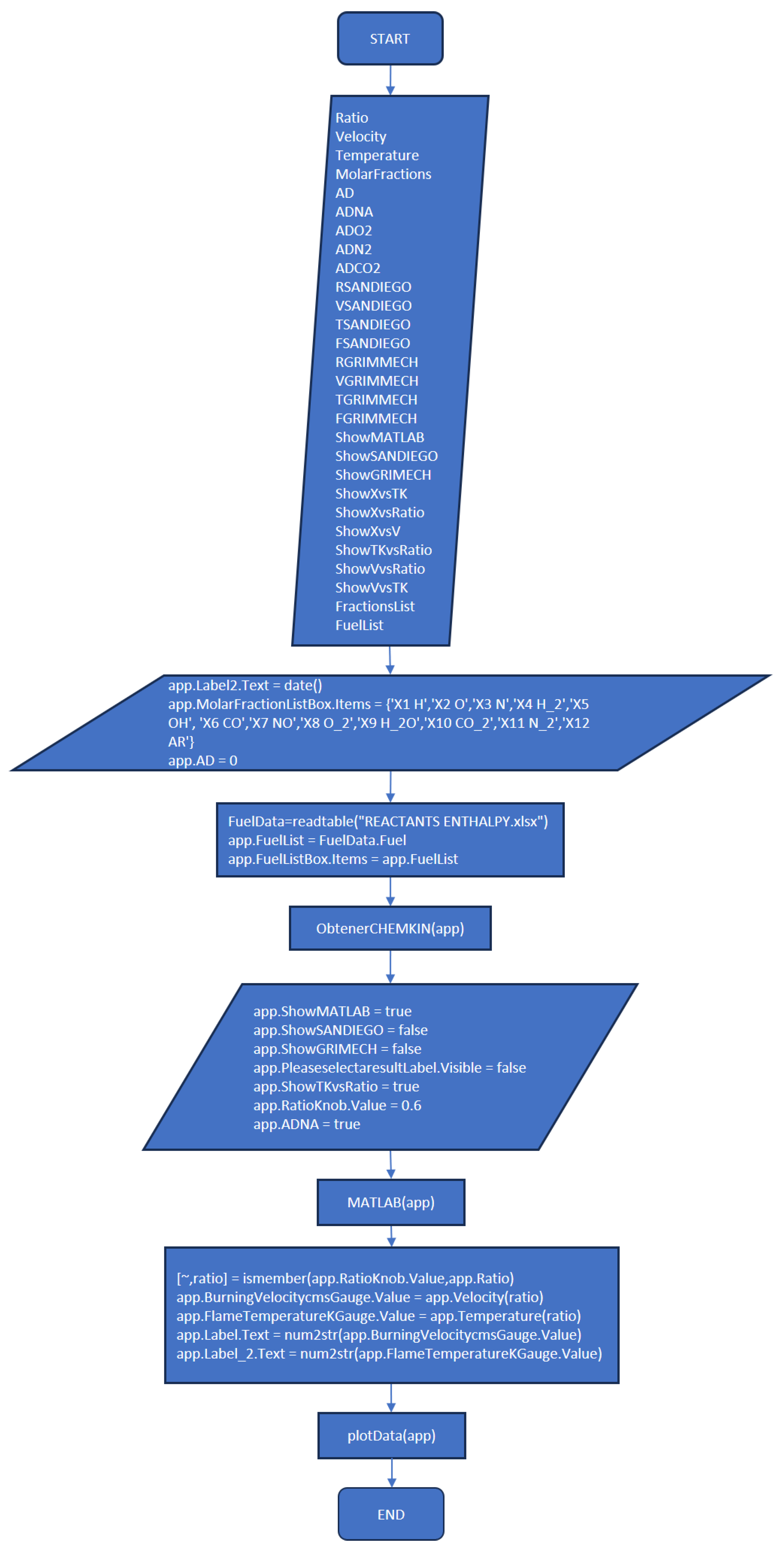
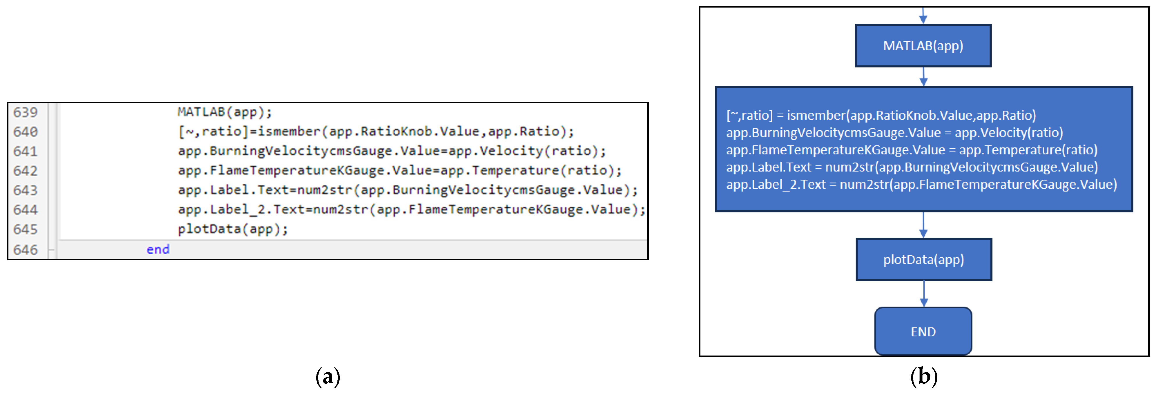
Finally, MATLAB function is called in order to obtain the results from the New_code.m and Fractions_Derivatives.m archives. In addition, the final gauges and tools labels are set with the result values and the function plotData is called for the purpose of creating the plot with the results obtained. This final part is shown in Figure 29.
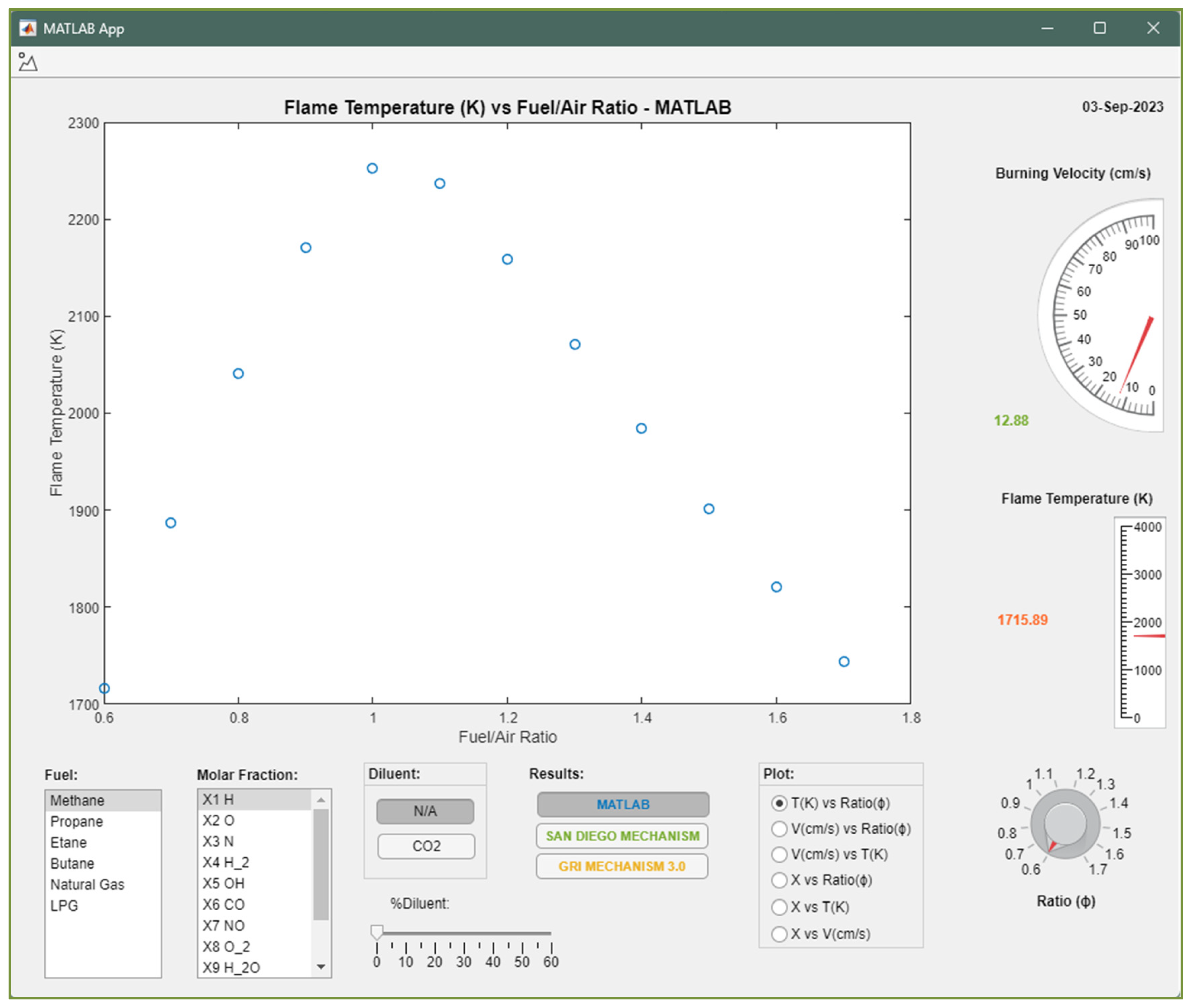
Finally, when the application is executed, the screen shown in Figure 30 will appear, and all the tools are identified and explained in Table 1.

4. Results and Discussions

The results obtained by executing the MATLAB Application are presented for three fuels (methane, propane and natural gas). These are compared and a brief discussion of the differences between them is presented for each fuel. Furthermore, the results from the application and from other relevant bibliography are compared in order to analyze and the behavior of the numerical method.

4.1. Methane

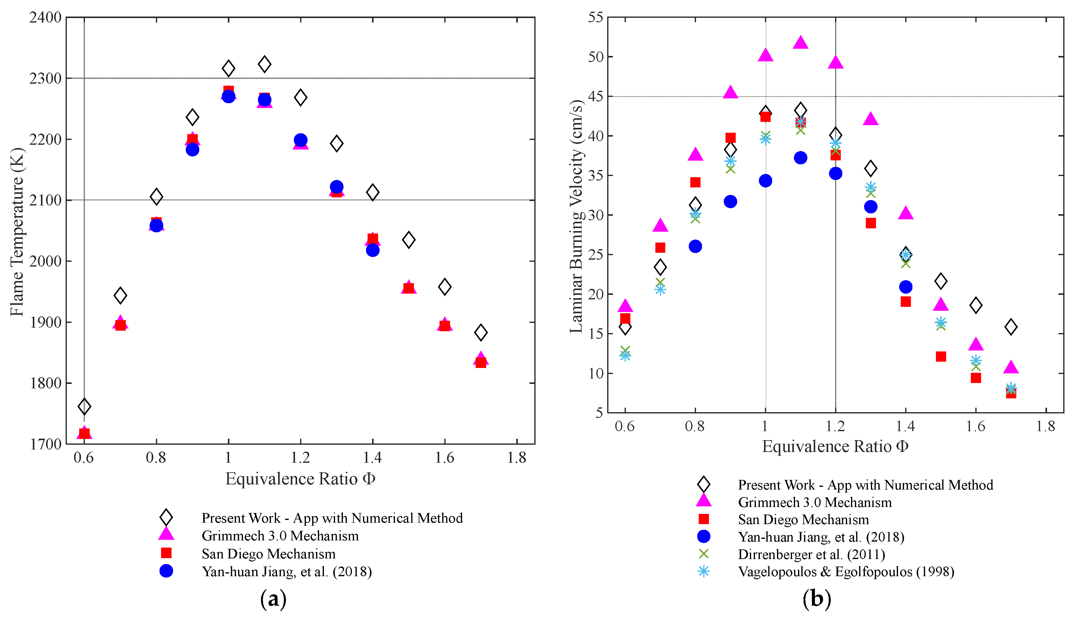
Figure 31 shows the results obtained for methane of flame temperature (a) and laminar burning velocity (b) compared with the research of Andrews and Bradley [11] and Sakhrieh [12].
From Figure 31, it is possible to affirm that the numerical method results have the same behavior as the two simulations in Ansys Chemkin (San Diego Mechanism [9] and GRI-MECH 3.0 [10]) and Andrews and Bradley’s bomb hot wire method study for flame temperature results [12]. For laminar burning velocity results, the work performed by Sakhrieh [12 is the most accurate one to the numerical method used while Andrews and Bradley’s [11] results are higher for mixtures near the stoichiometric.

4.2. Propane

Figure 32 shows the results obtained for propane of flame temperature (a) and laminar burning velocity (b) compared with Jiang, et al.’s research [13] and the investigation performed by Vagelopoulos and Egolfopoulos [14].
Figure 32 evidences that the numerical method flame temperature results have the same behavior as the two simulations in Ansys Chemkin (GRI-MECH 3.0 [10] and San Diego Mechanism [9]) and the numerical results from Jiang et al. [13]. However, in this case, the values for the numerical method using the MATLAB Application are considerably higher than the other resources. In addition, it is possible to observe that propane laminar burning velocity (cm/s) resulting from the numerical method has the same behavior as the other resources except the simulation using the GRI-MECH 3.0 in Ansys Chemkin whose values are higher than all the compared resources.

4.3. Natural Gas

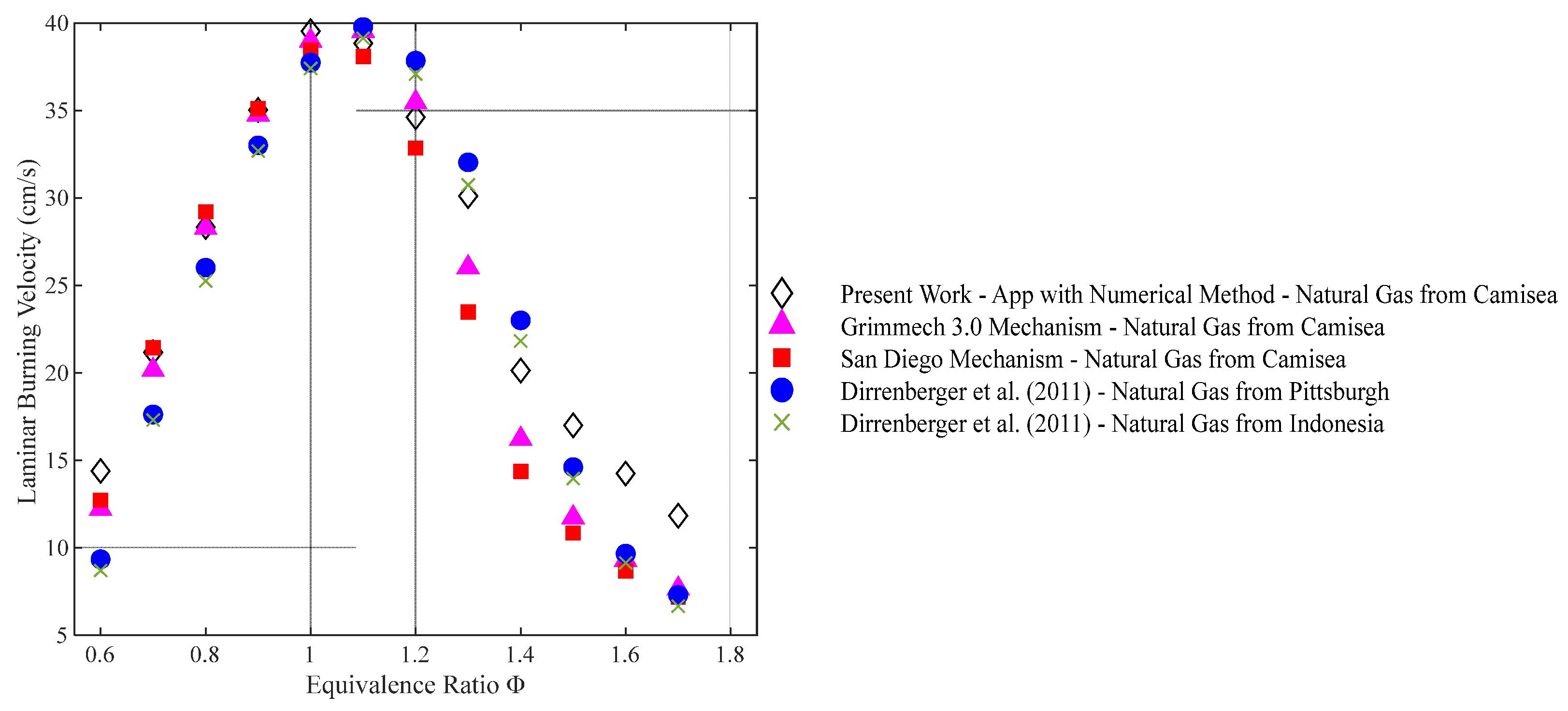
Figure 33 shows for natural gas the laminar burning velocity results from the present investigation (Camisea Natural Gas), Pittsburgh Gas and Indonesian Gas from Dirrenberger [15].
Figure 33 demonstrates that despite the different compositions of natural gas from the different resources (Camisea, Pittsburgh and Indonesian), the behavior of all the values (numerical method and simulations) are well matched for most of the cases of equivalence ratio, especially for poor and stoichiometric mixtures and near ones.

5. Conclusions

In this work, the numerical method coded in a MATLAB application for the determination of combustion characteristics (products of combustion, the adiabatic flame temperature and the laminar flame velocity) explanation and comparison with other resources was carried out. The following conclusions were reached:
  • In addition to the previously published article referenced as [8], the explanation provided in the present work completes the development plan and implementation of the MATLAB application.
  • The functions and execution sequence are described by using flowcharts and code extracts that allow everybody to understand how it works, and at the same time, the procedures are explicit for each part (New_code.m, Fractions_Derivatives.m, MATLAB_Application.mlapp), in order to provide the necessary information for future improvements.
  • With the MATLAB application, a functional and easy-to-use interface is obtained for the visualization and analysis of the results, whose program code (Code S1, Code S2 and Code S3) is available to modify in order to increase the fuel options (6 fuels by default), add more tools or to improve the whole methodology by adding more combustion products and new equations.
  • The implementation of the procedure for the determination of the laminar burning velocity as one of the novelties of this work is presented and explained as part of the New_code.m description that will allow users to improve the assumptions taken or include any other important variables not considered in the scope of the program.
  • The limitations of the application are: it can be only used for hydrocarbon fuels, which can have or not have oxygen and/or nitrogen; the flame temperature must not exceed 3725 °C and must be lower than 327 °C; and the equivalence ratio must not be too high so it does not allow the formation of free carbon [8].
  • The average execution time obtained by using the functions tic and toc in MATLAB when the application is initialized was 6.48 s, and when the fuel selection is changed (a new calculus is performed for the new selected fuel), it takes 6.18 s.

Supplementary Materials

The following supporting information can be downloaded at: https://doi.org/10.5281/zenodo.7894133, Code S1: New_code.m, File S1: REACTANTS EN THALPY.xlsx; File S2: DILUENTS ENTAHLPY.xlsx; Code S2: Fractions_Derivatives.m; Code S3: MATLAB_Application.mlapp. File S3: Ansys Chemkin Results.xlsx, File S4: Prod ucts.xlsx.

Author Contributions

Conceptualization, F.J.R.; methodology, R.F.C.; software, R.F.C.; validation, F.J.R.; investigation, R.F.C. and F.J.R.; resources, R.F.C.; writing—original draft, R.F.C.; writing—review and editing, F.J.R.; supervision, F.J.R.; project administration, F.J.R. All authors have read and agreed to the published version of the manuscript.

Funding

This research (PI0735) was funded by DFI PUCP.

Data Availability Statement

Not applicable.

Acknowledgments

Thanks are due to the DFI of the Pontificia Universidad Católica del Perú that, through the annual competition for applied research projects CAP PUCP 2021, financed research PI0735.

Conflicts of Interest

The authors declare no conflicts of interest.

Nomenclature

Fis the equivalence ratio
ADis the fraction of the diluent
IDis the identifier of the selected fuel;
ID2is the identifier of the selected diluent;
H_Datais the enthalpy of the fuel;
H_ADis the enthalpy of the diluent;
nis the carbon coefficient value of the fuel;
mis the hydrogen coefficient value of the fuel;
lis the oxygen coefficient value of the fuel;
kis the nitrogen coefficient value of the fuel;
AVMis the average molar mass
Eais the activation energy;
HRis the reactants enthalpy;
His the products enthalpy;
der_H_Tis the derivative of enthalpy respect temperature;
Tis the first assumed flame temperature or a temperature iteration;
Vis the laminar burning velocity
Xis the matrix of combustion products
x1is the molar fraction of Hydrogen (H) in the products;
x2is the molar fraction of Oxygen (O) in the products;
x3is the molar fraction of Nitrogen (N) in the products;
x4is the molar fraction of Hydrogen (H2) in the products;
x5is the molar fraction of Hydroxide (OH) in the products;
x6is the molar fraction of Carbon monoxide (CO) in the products;
x7is the molar fraction of Nitric oxide (NO) in the products;
x8is the molar fraction of Oxygen (O2) in the products;
x9is the molar fraction of Dihydrogen oxide (H2O) in the products;
x10is the molar fraction of Carbon dioxide (CO2) in the products;
x11is the molar fraction of Nitrogen (N2) in the products;
x12is the molar fraction of Argon (Ar) in the products;
x13is the number of moles from fuel that gives 1 mol of products;
Pis the pressure;
Kpis the equilibrium constants at constant pressure;
Tais the temperature for adjusting Kp;
PARfirst estimated value of x13;
fis the general linear function composed by 4 constants (F1, F2, F3 and F4);
F1is the first constant of f equation;
F2is the second constant of f equation;
F3is the third constant of f equation;
F4is the fourth constant of f equation;
dfis the differential equation of f;
oxis the first estimate value of x8
foxis the result of using ox as input in f;
dfoxis the result of using ox as input in df;
Bjis the matrix equations system of molar products;
new iterationis the variable that determines if a new iteration is required;
SMis the molar mass dataset;
HTis the enthalpy dataset;
CTis the specific heat capacity dataset;
DCTis the matrix of derivatives respect temperature;
DCPis the matrix of derivatives respect pressure;
DD4Fis the matrix of derivatives respect ratio;
C1is the equation matrix system formed by the derivatives;
Tkis the temperature used as input for calculate the specific enthalpy of a product;
ITis the fixed temperature to 0 decimals;
FRis the fraction part of the temperature;
SHis the matrix of specific enthalpy of each product;
CPis the constant pressure heat;
Label2is the label that shows current date;
app.ADis the value of diluent in the app;
app.ShowMATLABis the variable that shows MATLAB numerical method results;
app.ShowSANDIEGOis the variable that shows Ansys Chemkin using San Diego mechanism results;
app.ShowGRIMMECHis the variable that shows Ansys Chemkin using Grim 3.0 mechanism results;
app.PleaseselectaresultLabelis the variable that shows a message requiring the user to select a type of plot to shown on the application;
app.RatioKnobis the value set of the ratio knob

Appendix A

Figure A1. New_code.m flowchart.
Computation 12 00189 g0a1
Figure A2. Fractions_derivatives flowchart: (a) Part 1, (b), Part 2, (c) Part 3, (d) Part 4, (e) Part 5.
Computation 12 00189 g0a2aComputation 12 00189 g0a2bComputation 12 00189 g0a2cComputation 12 00189 g0a2dComputation 12 00189 g0a2e
Figure A3. MATLAB_Application.mlapp initialize flowchart.
Computation 12 00189 g0a3

References

  1. Zhu, D.L.; Egolfopoulos, F.N.; Law, C.K. Experimental and numerical determination of laminar flame speeds of methane/(Ar, N2, CO2)-air mixtures as function of stoichiometry, pressure, and flame temperature. Symp. (Int.) Combust. 1989, 22, 1537–1545. [Google Scholar] [CrossRef]
  2. Qin, W.; Egolfopoulos, F.N.; Tsotsis, T.T. Fundamental and environmental aspects of landfill gas utilization for power generation. Chem. Eng. J. 2001, 82, 157–172. [Google Scholar] [CrossRef]
  3. Hu, E.; Fu, J.; Pan, L.; Jiang, X.; Huang, Z.; Zhang, Y. Experimental and numerical study on the effect of composition on laminar burning velocities of H2/CO/N2/CO2/air mixtures. Int. J. Hydrogen Energy 2012, 37, 18509–18519. [Google Scholar] [CrossRef]
  4. Xiang, L.; Chu, H.; Ren, F.; Gu, M. Numerical analysis of the effect of CO2 on combustion characteristics of laminar premixed methane/air flames. J. Energy Inst. 2019, 92, 1487–1501. [Google Scholar] [CrossRef]
  5. Xie, M.; Fu, J.; Zhang, Y.; Shu, J.; Ma, Y.; Liu, J.; Zeng, D. Numerical analysis on the effects of CO2 dilution on the laminar burning velocity of premixed methane/air flame with elevated initial temperature and pressure. Fuel 2020, 264, 116858. [Google Scholar] [CrossRef]
  6. Ansys, Inc. Chemkin-Pro 19.0 Theory Manual; Ansys, Inc.: Canonsburg, PA, USA, 2018. [Google Scholar]
  7. Olikara, C.; Borman, G.L. A Computer Program for Calculating Properties of Equilibrium Combustion Products with Some Applications to I. C. Engines. In Proceedings of the 1975 Automotive Engineering Congress and Exposition, SAE International, Detroit, MI, USA, 24–28 February 1975. [Google Scholar] [CrossRef]
  8. Cisneros, R.F.; Rojas, F.J. Determination of 12 Combustion Products, Flame Temperature and Laminar Burning Velocity of Saudi LPG Using Numerical Methods Coded in a MATLAB Application. Energies 2023, 16, 4688. [Google Scholar] [CrossRef]
  9. Combustion, R. San Diego Mechanism Web Page, Chemical-Kinetic Mechanisms for Combustion Applications, San Diego Mechanism Web Page. Available online: http://combustion.ucsd.edu (accessed on 8 June 2023).
  10. GRI-MECH 3.0. Available online: http://www.me.berkeley.edu/gri_mech/ (accessed on 8 June 2023).
  11. Bradley, D.; Hundy, G.F. Burning velocities of methane-air mixtures using hot-wire anemometers in closed-vessel explosions. Symp. (Int.) Combust. 1971, 13, 575–583. [Google Scholar] [CrossRef]
  12. Sakhrieh, A. The adiabatic flame temperature and laminar flame speed of methane premixed flames at varying pressures. Acta Period. Technol. 2019, 50, 220–227. [Google Scholar] [CrossRef]
  13. Jiang, Y.-H.; Li, G.-X.; Li, H.-M.; Li, L.; Tian, L.-L.; Huang, H.-T. Experimental and Numerical Study on the Combustion Characteristics of Propane/Air Laminar Premixed Flame at Elevated Pressure. Energy Fuels 2018, 32, 9898–9907. [Google Scholar] [CrossRef]
  14. Vagelopoulos, C.M.; Egolfopoulos, F.N. Direct experimental determination of laminar flame speeds. Symp. (Int.) Combust. 1998, 27, 513–519. [Google Scholar] [CrossRef]
  15. Dirrenberger, P.; Le Gall, H.; Bounaceur, R.; Herbinet, O.; Glaude, P.; Konnov, A.; Battin-Leclerc, F. Measurements of Laminar Flame Velocity for Components of Natural Gas. Energy Fuels 2011, 25, 3875–3884. [Google Scholar] [CrossRef]
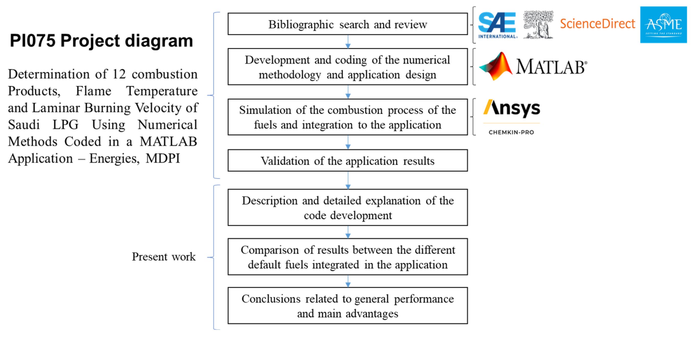
Figure 1. Methodology for the present work.
Computation 12 00189 g001
Figure 2. Initial verification of fuel ID and lecture of properties in New_code.m: (a) Code line, (b) Flowchart.
Computation 12 00189 g002
Figure 3. Determination of the fuel enthalpy in New_code.m: (a) Code line, (b) Flowchart.
Computation 12 00189 g003aComputation 12 00189 g003b
Figure 4. Determination of the air enthalpy and whole reactants enthalpy: (a) Code line, (b) Flowchart.
Computation 12 00189 g004
Figure 5. Definition of the activation energy, first estimate temperature, pressure and variables for the iteration process: (a) Code line, (b) Flowchart.
Computation 12 00189 g005
Figure 6. Iteration process for the determination of the product fractions, flame temperature and laminar burning velocity: (a) Code line, (b) Flowchart.
Computation 12 00189 g006
Figure 7. First definitions and verification of the initial defined estimated temperature: (a) Code line, (b) Flowchart.
Computation 12 00189 g007
Figure 8. Definition and determination of constants and verification of the equivalent ratio: (a) Code line, (b) Flowchart.
Computation 12 00189 g008
Figure 9. Definition of the equilibrium constants at constant pressure (Kp): (a) Code line, (b) Flowchart.
Computation 12 00189 g009
Figure 10. First estimation of ‘PAR’ (X13), the definition of ‘df’ and ‘ox’ variables for Newton–Raphson iteration process: (a) Code line, (b) Flowchart.
Computation 12 00189 g010aComputation 12 00189 g010b
Figure 11. Newton–Raphson method: (a) Code line, (b) Flowchart.
Computation 12 00189 g011aComputation 12 00189 g011b
Figure 12. Definition of equations for the other combustion products and their derivatives for matrix equation system: (a) Code line, (b) Flowchart.
Computation 12 00189 g012
Figure 13. Resolution of the matrix equation system by Gaussian elimination method using row interchange: (a) Code line, (b) Flowchart.
Computation 12 00189 g013
Figure 14. Final verification of the existence of a singular matrix in the matrix system: (a) Code line, (b) Flowchart.
Computation 12 00189 g014
Figure 15. Verification of the results tolerance and final calculation of the products: (a) Code line, (b) Flowchart.
Computation 12 00189 g015
Figure 16. Recalculation of variables for post operations procedure: (a) Code line, (b) Flowchart.
Computation 12 00189 g016
Figure 17. Introduction of properties and products data to the program: (a) Code line, (b) Flowchart.
Computation 12 00189 g017
Figure 18. Definition of derivatives respect temperature, pressure and ratio: (a) Code line, (b) Flowchart.
Computation 12 00189 g018
Figure 19. Resolution of the matrix equation system by Gaussian elimination method using maximum pivot strategy: (a) Code line, (b) Flowchart.
Computation 12 00189 g019
Figure 20. Verification of the existence of a singular matrix in the system: (a) Code line, (b) Flowchart.
Computation 12 00189 g020aComputation 12 00189 g020b
Figure 21. Recalculation of partial derivatives: (a) Code line, (b) Flowchart.
Computation 12 00189 g021
Figure 22. Determination of the single row matrix SH: (a) Code line, (b) Flowchart.
Computation 12 00189 g022
Figure 23. Determination of average molar mass (AVM) and products enthalpy: (a) Code line, (b) Flowchart.
Computation 12 00189 g023
Figure 24. Determination of CP and partial derivative of enthalpy respect temperature: (a) Code line, (b) Flowchart.
Computation 12 00189 g024
Figure 25. Properties definition in the application: (a) Code line, (b) Flowchart.
Computation 12 00189 g025
Figure 26. Definition of molar fraction list items: (a) Code line, (b) Flowchart.
Computation 12 00189 g026
Figure 27. Definition of the fuel list and lecture of the Ansys Chemkin simulations results: (a) Code line, (b) Flowchart.
Computation 12 00189 g027
Figure 28. Setting of the variables for plotting: (a) Code line, (b) Flowchart.
Computation 12 00189 g028
Figure 29. MATLAB and plot functions: (a) Code line, (b) Flowchart.
Computation 12 00189 g029
Figure 30. Application first screen with identified tools [8].
Computation 12 00189 g030
Figure 31. Results comparison with references [11,12] for Methane: (a) Flame temperature (K) versus equivalence ratio, (b) Laminar burning velocity (cm/s) versus equivalence ratio.
Computation 12 00189 g031
Figure 32. Results comparison for Propane: (a) Flame temperature (K) versus equivalence ratio, (b) Laminar burning velocity versus equivalence ratio compared with references [13,14].
Computation 12 00189 g032
Figure 33. Results comparison with research referenced as [15] for different compositions of Natural Gas Laminar burning velocity versus equivalence ratio.
Computation 12 00189 g033
Table 1. Tools available in the MATLAB Application [8].
PositionName of ToolDescriptionSelection Type
AFuel listList of fuels available for calculus in the applicationUnique
BMolar fraction listList of molar fractions available for plotting resultsUnique
CDiluent button listList of diluents available to use in calculusUnique
DPercentage bar of diluentPercentage of diluent by volume to be considered in fuelUnique
EResults button listResults from resources available to be show in the plotMulti
FPlot button listType of plot to be show in the screenUnique
GEquivalence ratio knobKnob that allows to see the value of laminar burning velocity and flame temperature in their respective gaugesUnique
HLaminar burning velocity gaugeLaminar burning velocity value at the knob equivalence ratio value selectedNA
IFlame temperature gaugeFlame temperature value at the knob equivalence ratio value selected.NA
Disclaimer/Publisher’s Note: The statements, opinions and data contained in all publications are solely those of the individual author(s) and contributor(s) and not of MDPI and/or the editor(s). MDPI and/or the editor(s) disclaim responsibility for any injury to people or property resulting from any ideas, methods, instructions or products referred to in the content.