Quadrotor Trajectory Tracking Using Model Reference Adaptive Control, Neural Network-Based Parameter Uncertainty Compensator, and Different Plant Parameterizations

Abstract

A quadrotor trajectory tracking problem is addressed via the design of a model reference adaptive control (MRAC) system. As for real-world applications, the entire quadrotor dynamics is typically unknown. To take that into account, we consider a plant model, which contains uncertain nonlinear terms resulting from aerodynamic friction, blade flapping, and the fact that the mass and inertia moments of the quadrotor may change from their nominal values. Unlike many known studies, the explicit equations of the parameter uncertainty for the position control loop are derived in two different ways using the differential flatness approach: the control signals are (i) used and (ii) not used in the parametric uncertainty parameterization. After analysis, the neural network (NN) is chosen for both cases as a compensator of such uncertainty, and the set of NN input signals is justified for each of them. Unlike many known MRAC systems with NN for quadrotors, in this study, we use the $k_{x}x+k_{r}r$ baseline controller, which follows from the control system derivation, with both time-invariant (parameterization (i)) and adjustable (parameterization (ii)) parameters instead of an arbitrarily chosen non-tunable PI/PD/PID-like one. Adaptive laws are derived to adjust the parameters of NN uncertainty compensator for both parameterizations. As a result, the position controller ensures the asymptotic stability of the tracking error for both cases under the assumption of perfect attitude loop tracking, which is ensured in the system previously developed by the authors. The results of the numerical experiments support the theoretical conclusions and provide a comparison of the effectiveness of the derived parameterizations. They also allow us to make conclusions on the necessity of the baseline controller adjustment.

1. Introduction

This study is an extended version of a previously published conference paper [1].

The problem of quadrotor control quality improvement under the condition of parameter uncertainty has gained considerable attention from the control community in the recent years [2] because of the numerous outdoor and indoor civilian applications of such devices in the following: agriculture, traffic monitoring, delivery, mapping coverage, etc.

The main advantages of the quadrotors are their small size, light weight, vertical take-off and landing, and dynamical maneuverability. However, on the other hand, their dynamics is non-linear with couplings between translational and rotational motions; we have only four control signals (thrust and rotational torques) for six degrees of freedom. Moreover, some parameters of such a plant can not be known precisely: aerodynamical coefficients, its mass, and inertia moments. For instance, if the quadrotor is spraying pesticides on crops, its mass is getting lower like a smooth function, while in the case of cargo delivery, such variation happens in a step-like manner. It should be noted that the inertia moments change their values in both cases.

Despite all the above-mentioned difficulties, the quadrotor position control is required to be of high quality, especially if the indoor missions are considered. To solve such a complicated problem, the control system is usually implemented in accordance with the cascade principle [3] with the inner attitude and outer position loops. The plants of both have their own parameter uncertainties to be compensated. The scope of this research is the position loop only, but interested readers are referred to [4], in which a short review of the existing methods of attitude adaptive control is given, and an effective solution of such problem is proposed.

As far as the trajectory tracking is concerned, the following different techniques have been applied to solve the control problem under consideration: the conventional PID-control [5], LQ-regulator [5,6], backstepping [7], and feedback linearization [8]. However, all of them require the plant dynamics (model parameters) to be known a priori.

To relax such a strict requirement, two solutions should be mentioned. The first is an active disturbance rejection control [9], which is based on the idea of the disturbance (uncertainty) estimation with the help of the extended state observer (ESO). It is a linear high-gain observer, in which the large gain may induce the well-known peaking phenomenon. So, such a scheme is not considered further.

Secondly, the adaptive control techniques can be applied. In particular, the model reference adaptive control (MRAC) with the conventional adaptive law of the form of $-\Gamma e_{ref}PBx$ is used in [10]. Unfortunately, it is not explained why the baseline controller is chosen as the PD instead of $k_{x}x+k_{r}r$, as well as the absence of the $\sigma$ or e robust modification in the adaptive law to compensate for the parameter uncertainty, given that its basis functions are approximated using the set of radial-basis ones. The presented stability analysis of such a scheme holds only in case the uncertainty parameters are time invariant.

As the parameter uncertainty is both time varying and nonlinear, it is worth applying the universal approximators such as neural networks (NN) to compensate for it. NN is used to implement compensators in the MRAC-like robust scheme with a PD-based baseline controller [11] and the schemes of backstepping in [12,13]. The solution from [11] requires the known upper bounds of some constituent parts of the parameter uncertainty, while the application of backstepping results in complex controllers of a high dynamic order. Concerning NNs in [11,12,13], the input vector components are chosen without analysis of what signals form the uncertainty to be compensated, and only the output layer parameters are adjusted. So, the higher number of hidden neurons is to be chosen to obtain the required approximation error [14]. More detailed analyses of NN applications to solve the problem under consideration can be found in recent studies [15,16]. As for [15,16], the proposed solutions use the PI/PID controller with time-invariant parameters as a baseline, which contradicts the classical principles of MRAC system synthesis.

All in all, despite a great number of studies on the application of MRAC + NN to control quadrotor trajectory, all of them contains at least some of the following disadvantages:

(d1)

A simplified model of the quadrotor with time-invariant parameters of mass and inertia moments is used.

(d2)

The explicit equation of the parameter uncertainty to be compensated is not presented, as well as the numerical simulation results, which compare the outputs of the proposed compensator with the ones of such equation. This makes it difficult to understand to what extent the uncertainty has been compensated.

(d3)

The baseline controller is chosen arbitrarily but not as a result of the synthesis procedure.

(d4)

Baseline controller has time-invariant parameters, and plant parameterization, under which it can also be adjustable, is not considered.

This study fills this gap and designs the direct MRAC schemes with the NN-based compensator of matched parameter uncertainty for a quadrotor, which are free from the above-mentioned disadvantages.

The following contributions of this study are that simultaneously:

(c1)

The explicit equations of the parameter uncertainty are derived for the quadrotor trajectory tracking problem for two cases, when control signals are (i) used and (ii) not used in the parametric uncertainty parameterization;

(c2)

Using (c1), the application of NN-based uncertainty compensator and signals included into its input vector are justified;

(c3)

The MRAC-based schemes are implemented with the baseline controller of a $k_{x}x+k_{r}r$ type (in two variants, with time-invariant and adjustable $k_x$ and $k_r$) and the NN-based compensator of the paramtric uncertainty, in which the parameters of both output and hidden layers are adjusted in real time.

2. Problem Statement and Methods

2.1. Mathematical Model of Quadrotor

Schematic representation of quadrotor is shown in Figure 1.

The equations of the quadrotor model [8] are written as follows (the brackets and the time argument are omitted whenever it is clear from the context and causes no confusion):

$$\begin{array}{c}\dot{\overline{p}}=\overline{V}=R{V}^b,\dot{\xi }=\omega =J{\omega }^b,\\ {\dot{V}}^b=\frac{1}{m}{F}_{ext}-{\omega }^b\times V^b,I_b{\dot{\omega }}_b={\tau }_{ext}-{\omega }^b\times I_b{\omega }^b,\end{array}$$

(1)

where m is a plant mass, $\psi$ is roll, $\theta$ stands for pitch, and $\varphi$ denotes yaw, $\xi ={\left[\begin{array}{c}\psi ,\theta ,\varphi \end{array}\right]}^{\mathrm{T}}$. The center of gravity of the quadrotor is the origin of a body-fixed frame (BFF). Considering the inertial frame (IF), $\overline{p}=\left(X,Y,Z\right)$ is the coordinate vector, $\overline{V}={\left[\begin{array}{ccc}\dot{X}& \dot{Y}& \dot{Z}\end{array}\right]}^{\mathrm{T}}$ stands for the linear velocity, and $w={\left[\begin{array}{ccc}\dot{\psi }& \dot{\theta }& \dot{\varphi }\end{array}\right]}^{\mathrm{T}}$ is the plant angular velocity. As far as the BFF is concerned, the same vectors are denoted as ${\overline{p}}^b=(x,y,z)$, $V^b={\left[\begin{array}{c}u,v,\mathrm{w}\end{array}\right]}^{\mathrm{T}}$, and ${\omega }^b={\left[\begin{array}{c}p,q,r\end{array}\right]}^{\mathrm{T}}$, respectively. $F_{ext}={\left[\begin{array}{c}{f}_x,f_y,f_z\end{array}\right]}^{\mathrm{T}}$ and ${\tau }_{ext}={\left[\begin{array}{c}{\tau }_{\psi },{\tau }_{\theta },{\tau }_{\varphi }\end{array}\right]}^{\mathrm{T}}$ are the external forces and moments in BFF. ${\tau }_{\psi },{\tau }_{\theta },{\tau }_{\varphi }$ are calculated via $\psi$, $\theta$, and $\varphi$ controllers. R and J are transformation matrices, which are expressed as follows:

$$\begin{array}{c}R=\left[\begin{array}{ccc}{c}_{\theta }{c}_{\varphi }& s_{\psi }{s}_{\theta }{c}_{\varphi }-c_{\psi }{s}_{\varphi }& c_{\psi }{s}_{\theta }{c}_{\varphi }+s_{\psi }{s}_{\varphi }\\ c_{\theta }{s}_{\varphi }& s_{\psi }{s}_{\theta }{s}_{\varphi }+c_{\psi }{c}_{\varphi }& c_{\psi }{s}_{\theta }{s}_{\varphi }-s_{\psi }{c}_{\varphi }\\ -s_{\theta }& s_{\psi }{c}_{\theta }& c_{\psi }{c}_{\theta }\end{array}\right],\end{array}\begin{array}{c}J=\left[\begin{array}{ccc}1& s_{\psi }{t}_{\theta }& c_{\psi }{t}_{\theta }\\ 0& c_{\psi }& -s_{\psi }\\ 0& s_{\psi }/c_{\theta }& c_{\psi }/c_{\theta }\end{array}\right],\end{array}$$

(2)

Hereafter, $s_{(.)}$ stands for $sin(.)$, $c_{(.)}$ is $cos(.)$, and $t_{(.)}$ denotes $tan(.)$.

Assumption 1.

The inertia matrix $I_b=diag(J_x,J_y,J_z)$ is diagonal as the quadrotor is symmetric in $xB-zB$ and $yB-zB$ planes.

Taking into account the drag force [8], Equation (1) are represented as follows:

$$\begin{array}{c}\left[\begin{array}{c}\dot{X}\\ \dot{Y}\\ \dot{Z}\end{array}\right]=R\left[\begin{array}{c}u\\ v\\ w\end{array}\right],\left[\begin{array}{c}\dot{\psi }\\ \dot{\theta }\\ \dot{\varphi }\end{array}\right]=J\left[\begin{array}{c}p\\ q\\ r\end{array}\right],\end{array}$$

(3)

$$\begin{array}{c}\left[\begin{array}{c}\dot{p}\\ \dot{q}\\ \dot{r}\end{array}\right]=\left[\begin{array}{c}qr\frac{J_y-J_z}{J_x}\\ pr\frac{J_z-J_x}{J_y}\\ pq\frac{J_x-J_y}{J_z}\end{array}\right]+\underset{{\Delta }_{pqr}}{\underbrace{\left[\begin{array}{c}q{\omega }_r\frac{J_r}{J_x}-\dot{\psi }\frac{k_{\psi }l}{J_x}-s_{\psi }\frac{K_c}{J_x}\\ -p{\omega }_r\frac{J_r}{J_y}-\dot{\theta }\frac{k_{\theta }l}{J_y}-s_{\theta }\frac{K_c}{J_y}\\ -\dot{\varphi }\frac{k_{\varphi }l}{J_z}\end{array}\right]}}+\left[\begin{array}{c}\frac{{\tau }_{\psi }}{J_x}\\ \frac{{\tau }_{\theta }}{J_y}\\ \frac{{\tau }_{\varphi }}{J_z}\end{array}\right],\end{array}$$

(4)

$$\left[\begin{array}{c}\dot{u}\\ \dot{v}\\ \dot{w}\end{array}\right]=\left[\begin{array}{c}rv-qw\\ pw-ru\\ qu-pv\end{array}\right]+\left[\begin{array}{c}g{s}_{\theta }\\ -g{c}_{\theta }{s}_{\psi }\\ -g{c}_{\theta }{c}_{\psi }+\frac{T}{m}\end{array}\right]+\underset{{\Delta }_{uvw}}{\underbrace{\left[\begin{array}{c}\frac{-C_x\rho S_{x}u\left|u\right|}{2m}\\ \frac{-C_y\rho S_{y}v\left|v\right|}{2m}\\ \frac{-C_z\rho S_{z}w\left|w\right|}{2m}\end{array}\right]}},$$

(5)

where $K_c,C_x,C_y,C_z$ stand for aerodynamic coefficients; $k_{\psi }$, $k_{\theta }$ are the air resistance parameters; $\rho$ is the air density; $S_x,S_y,S_z$ are the quadrotor surface areas corresponding to the respective axis; l is the distance between the gravity center and each motor rotor; $J_r$ stands for the inertia moment of the motor; and ${\omega }_r$ is the total motors speed.

The output of the altitude controller is T. Lift forces $T_1,T_2,T_3,T_4$ and rotational torques $M_1,M_2,M_3,M_4$ are calculated from $T,{\tau }_{\psi },{\tau }_{\theta },{\tau }_{\varphi }$, using (13) from [8].

2.2. Trajectory Tracking Control Problem

Assumption 2.

The parameters values of the quadrotor model are unknown. $p,q,r$ and $u,v,w$ are measurable. Then, all other states from (3)–(5) can be obtained.

Assumption 3.

The inner attitude control system that includes $\psi ,\theta ,\varphi$ loops has already been designed using the approach from [4]. That means that despite (a) $J_x,J_y,J_z$ being unknown and time-varying and (b) having ${\Delta }_{pqr}$ in (4) and J in the right-hand part of (3), the NN-based compensator of the the inner loop proposed in [4] ensures $\psi ,\theta ,\varphi$ control quality defined using the attitude reference model.

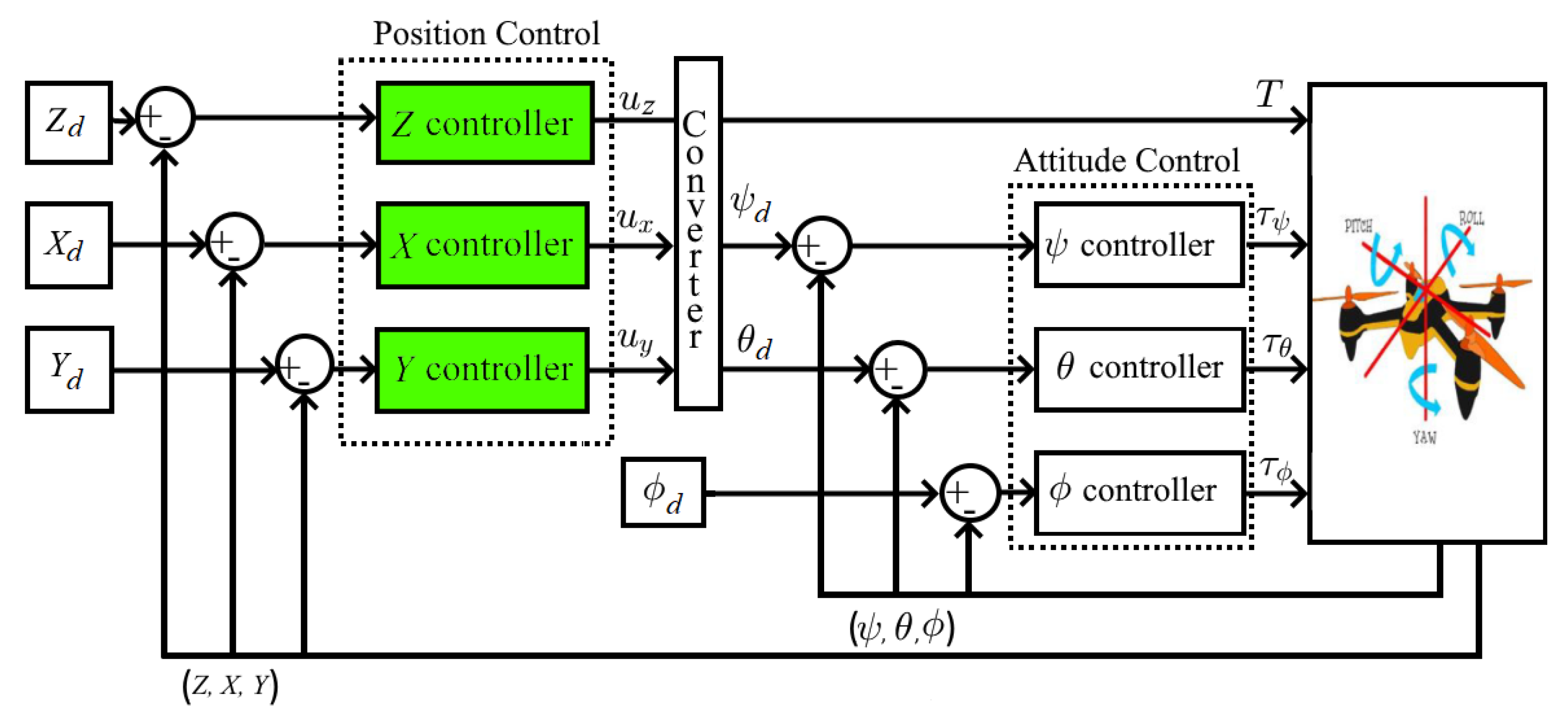
Goal. To solve the quadrotor trajectory tracking problem via development of MRAC system (green blocks in Figure 2), which is capable of the parameter uncertainty (see (5)) compensation and ensures asymptotic convergence of the tracking error to a compact set.

3. Main Result

3.1. Uncertainty Parameterization

The left equation in (3) is differentiated with regards to time. The substitution of (5) into the obtained result yields the following:

$$\begin{array}{c}\left[\begin{array}{c}\ddot{X}\\ \ddot{Y}\\ \ddot{Z}\end{array}\right]=R\left[\begin{array}{c}\dot{u}\\ \dot{v}\\ \dot{w}\end{array}\right]+\dot{R}\left[\begin{array}{c}u\\ vs.\\ w\end{array}\right]=R\left[\begin{array}{c}0\\ 0\\ 1\end{array}\right]\frac{T}{m}+R\left[\begin{array}{c}rv-qw\\ pw-ru\\ qu-pv\end{array}\right]\\ +R\left[\begin{array}{c}g{s}_{\theta }\\ -g{c}_{\theta }{s}_{\psi }\\ -g{c}_{\theta }{c}_{\psi }\end{array}\right]+R{\Delta }_{uvw}+\dot{R}\left[\begin{array}{c}u\\ vs.\\ w\end{array}\right]=\left[\begin{array}{c}{c}_{\psi }{s}_{\theta }{c}_{\varphi }+s_{\psi }{s}_{\varphi }\\ c_{\psi }{s}_{\theta }{s}_{\varphi }-s_{\psi }{c}_{\varphi }\\ c_{\psi }{c}_{\theta }\end{array}\right]\frac{T}{m}\\ +\underset{\overline{\Delta }}{\underbrace{R\left[\begin{array}{c}rv-qw\\ pw-ru\\ qu-pv\end{array}\right]+R\left[\begin{array}{c}g{s}_{\theta }\\ -g{c}_{\theta }{s}_{\psi }\\ -g{c}_{\theta }{c}_{\psi }\end{array}\right]+R{\Delta }_{uvw}+\dot{R}\left[\begin{array}{c}u\\ vs.\\ w\end{array}\right]}},\end{array}$$

(6)

$$\dot{R}=R·\left[\begin{array}{ccc}0& -r& q\\ r& 0& -p\\ -q& p& 0\end{array}\right].$$

The actual quadrotor mass m is unknown and time varying. However, we know its nominal constant value $\overline{m}$.

The aim is to ensure trajectory tracking independent of the value of the yaw angle, i.e., $X_d,Y_d,Z_d$ are to be followed with the required quality at any value of $\varphi$. To achieve this, the differential flatness approach [17] is applied:

$$\begin{array}{c}{\theta }_d=arctan\left(\frac{1}{u_z}\left(u_x{c}_{\varphi }+u_y{s}_{\varphi }\right)\right),\hfill \\ {\psi }_d=arctan\left(c_{\theta }\frac{1}{u_z}\left(u_x{s}_{\varphi }-u_y{c}_{\varphi }\right)\right),T=\frac{\overline{m}{u}_z}{c_{\psi }{c}_{\theta }}.\end{array}$$

(7)

This equation is actually an implementation of the converter block in Figure 2.

Further parameterization depends on whether $u_x,u_y,u_z$ is directly used in the uncertainty parameterization or not.

3.1.1. Case I: Control Signals Are Directly Used in Uncertainty Parameterization

Equation (6) is rewritten as follows:

$$\begin{array}{c}\left[\begin{array}{c}\ddot{X}\\ \ddot{Y}\\ \ddot{Z}\end{array}\right]=\left[\begin{array}{c}{c}_{\psi }{s}_{\theta }{c}_{\varphi }+s_{\psi }{s}_{\varphi }\\ c_{\psi }{s}_{\theta }{s}_{\varphi }-s_{\psi }{c}_{\varphi }\\ c_{\psi }{c}_{\theta }\end{array}\right]\frac{T}{\overline{m}}+\left[\begin{array}{c}{c}_{\psi }{s}_{\theta }{c}_{\varphi }+s_{\psi }{s}_{\varphi }\\ c_{\psi }{s}_{\theta }{s}_{\varphi }-s_{\psi }{c}_{\varphi }\\ c_{\psi }{c}_{\theta }\end{array}\right]T\frac{\overline{m}-m}{m\overline{m}}+\overline{\Delta }.\end{array}$$

(8)

The only constant in (8) is $\overline{m}$.

Equation (7) is substituted into (8) to obtain the following:

$$\left[\begin{array}{c}\ddot{X}\\ \ddot{Y}\\ \ddot{Z}\end{array}\right]=\left[\begin{array}{c}{u}_x\\ u_y\\ u_z\end{array}\right]+\underset{\Delta }{\underbrace{\left[\begin{array}{c}{u}_x\\ u_y\\ u_z\end{array}\right]\frac{\overline{m}-m}{m}+\overline{\Delta }}}.$$

(9)

Therefore, $\Delta ={\left[\begin{array}{ccc}{\Delta }_X& {\Delta }_Y& {\Delta }_Z\end{array}\right]}^{\mathrm{T}}\in {\mathbb{R}}^{3\times 1}$ is the matched parameter uncertainty to be compensated. It can be rewritten as a linear regression with unknown m (time varying), $\rho$, $C_x$, $C_y$, $C_z$, $S_x$, $S_y$, $S_z$ and measurable nonlinear regressor, which depends on the twelve known signals $u_x,u_y,u_z,\psi ,\theta ,\varphi ,u,v,w,p,q,r$. The obtained parameterization has two main features: (i) the input gain matrix is known and identified, and (ii) control signals $u_x,u_y,u_z$ are included into uncertainty parameterization.

3.1.2. Case II: Control Signals Are Not Used in Uncertainty Parameterization

Equation (6) is used, and (7) is substituted into it as follows:

$$\left[\begin{array}{c}\ddot{X}\\ \ddot{Y}\\ \ddot{Z}\end{array}\right]=\left[\begin{array}{c}{u}_x\\ u_y\\ u_z\end{array}\right]\frac{\overline{m}}{m}+\overline{\Delta }=\frac{\overline{m}}{m}\left(\left[\begin{array}{c}{u}_x\\ u_y\\ u_z\end{array}\right]+\Delta \right).$$

(10)

In such a case, the matched parametric uncertainty again can be rewritten as a linear regression, but its regressor does not include $u_x,u_y,u_z$. Furthermore, the system input gain matrix is unknown and represented as a diagonal matrix with $\frac{\overline{m}}{m}$ on its main diagonal.

3.1.3. Representation of Plant in State-Space Form

The state $x_p={\left[X,\dot{X},Y,\dot{Y},Z,\dot{Z}\right]}^{\mathrm{T}}$ and control vectors $u={\left[u_x,u_y,u_z\right]}^{\mathrm{T}}$ are introduced. Then, (9) and (10) are written as follows:

$$\begin{array}{c}\dot{x}{}_p\left(t\right)=A_p{x}_p\left(t\right)+B_p\left(u\left(t\right)+\Delta \left(t\right)\right),\\ u\left(t\right)=u_{base}\left(t\right)-u_{ad}\left(t\right),\end{array}$$

(11)

Considering (9), we have the following:

$$\begin{array}{c}{B}_p=I_{3\times 3}\otimes \left[\begin{array}{c}0\\ 1\end{array}\right],A_p=I_{3\times 3}\otimes \left[\begin{array}{cc}0& 1\\ 0& 0\end{array}\right],\end{array}$$

while it is written for (10) as follows:

$$\begin{array}{c}{B}_p=\left(\underset{\Lambda }{\underbrace{\frac{\overline{m}}{m}}}{I}_{3\times 3}\right)\otimes \left[\begin{array}{c}0\\ 1\end{array}\right],A_p=I_{3\times 3}\otimes \left[\begin{array}{cc}0& 1\\ 0& 0\end{array}\right].\end{array}$$

$\Lambda$ is unknown. So, in the course of the following design, we will need $u_{base}$ with time-invariant parameters for Case I and adjustable ones for Case II.

The uncertainty $\Delta$ is time varying and has a nonlinear regressor for both cases, so NN is chosen to compensate for it.

3.2. MRAC System with NN-Based Compensator

3.2.1. Reference Model

The reference model is introduced as follows:

$$\begin{array}{c}{\dot{x}}_{ref}\left(t\right)=A_{ref}{x}_{ref}\left(t\right)+B_{ref}r\left(t\right),\\ B_{ref}=I_{3\times 3}\otimes \left[\begin{array}{c}0\\ {\mathfrak{w}}_n^2\end{array}\right],A_{ref}=I_{3\times 3}\otimes \left[\begin{array}{cc}0& 1\\ a_0& a_1\end{array}\right].\end{array}$$

(12)

The following definitions are used: $x_{ref}={\left[X_{ref},{\dot{X}}_{ref},Y_{ref},{\dot{Y}}_{ref},Z_{ref},{\dot{Z}}_{ref}\right]}^{\mathrm{T}}$, $r={\left[\begin{array}{ccc}{X}_d& Y_d& Z_d\end{array}\right]}^{\mathrm{T}}$, $a_0=-{\mathfrak{w}}_n^2$, $a_1=-2\mathfrak{g}{\mathfrak{w}}_n^{}$, $\mathfrak{g}>0$, ${\mathfrak{w}}_n>0$.

3.2.2. Plant Representation: Neural Network Description

According to the proved approximation theorem [18], $\Delta$ is expressed as NN with the sigmoid activation function $\sigma$ in the hidden layer (Figure 3) as follows:

$$\begin{array}{c}{\dot{x}}_p=A_p{x}_p+B_p\left(u+\underset{{\Delta }^{★}}{\underbrace{W^{\mathrm{T}}\sigma \left(V^{\mathrm{T}}{x}_{nn}\right)}}+\epsilon \right),\\ ∥\epsilon ∥\le {\epsilon }_N,x_{nn}={\left[\begin{array}{cccc}{b}^1& {\xi }^{\mathrm{T}}& {\left(V^b\right)}^{\mathrm{T}}& {\left({\omega }^b\right)}^{\mathrm{T}}\end{array}\right]}^{\mathrm{T}},\\ \sigma \left(V^T{x}_{nn}\right)={\left[\begin{array}{ccccc}{b}^2& {\sigma }_1& {\sigma }_2& \cdots & {\sigma }_{N2}\end{array}\right]}^{\mathrm{T}},\\ V=\left[\begin{array}{ccc}{\beta }_1^1& \cdots & {\beta }_{N2}^1\\ {\omega }_{1,1}^1& \cdots & {\omega }_{1,N2}^1\\ ⋮& \ddots & ⋮\\ {\omega }_{N1,1}^1& \cdots & {\omega }_{N1,N2}^1\end{array}\right],W=\left[\begin{array}{ccc}{\beta }_1^2& \cdots & {\beta }_{N3}^2\\ {\omega }_{1,1}^2& \cdots & {\omega }_{1,N3}^2\\ ⋮& \ddots & ⋮\\ {\omega }_{N2,1}^2& \cdots & {\omega }_{N2,N3}^2\end{array}\right].\end{array}$$

On the basis of the obtained parameter uncertainty parameterization, it is concluded that the number of the input neurons is $N_1=12$ for Case I ($x_{nn}=\{u_x,u_y,u_z,\psi ,\theta ,\varphi ,u$, $v,w,p,q,r\}$) and $N_1=9$ ($x_{nn}=\{\psi ,\theta ,\varphi ,u,v,w,p,q,r\}$) for Case II, the number of output neurons is $N_3=3$ for both cases. $\epsilon$ is the approximation error, of which its upper bound ($∥\epsilon ∥\le {\epsilon }_N$) can be estimated using the results from [14]. It depends on the number of hidden neurons $N_2$, the higher $N_2$, and the lower ${\epsilon }_N$.

As ideal weights W and V are unknown, NN with adjustable parameters $\widehat{V}$ and $\widehat{W}$ is introduced as follows [19]:

$$\begin{array}{c}\widehat{\Delta }={\widehat{W}}^{\mathrm{T}}\sigma \left({\widehat{V}}^{\mathrm{T}}{x}_{nn}\right),\end{array}$$

(13)

The adaptive laws for $\widehat{V}$ and $\widehat{W}$ will be derived further for both cases under consideration.

3.2.3. MRAC System Design

The approximation and estimation errors are introduced as follows:

$$\begin{array}{c}e=\Delta -{\Delta }^{★}-\epsilon ,\\ \tilde{V}=\widehat{V}-V,\tilde{W}=\widehat{W}-W.\end{array}$$

(14)

The dependence of e from V is nonlinear due to the sigmoid function, so it is linearized via the Taylor series expansion as follows:

$$\begin{array}{c}\sigma \left(V^{\mathrm{T}}{x}_{nn}\right)=\sigma \left({\widehat{V}}^{\mathrm{T}}{x}_{nn}\right)-\dot{\sigma }\left({\widehat{V}}^{\mathrm{T}}{x}_{nn}\right){\tilde{V}}^{\mathrm{T}}{x}_{nn}+O{\left({\tilde{V}}^{\mathrm{T}}{x}_{nn}\right)}^2.\end{array}$$

(15)

Introducing $e_{ref}=x_p-x_{ref}$, the error equation is obtained as follows:

$$\begin{array}{c}{\dot{e}}_{ref}=A_{ref}{e}_{ref}+B_p\left(-u_{ad}+{\Delta }^{★}+\epsilon \right)+B_p\left(u_{base}-B_p^{†}{B}_{ref}r+B_p^{†}\left(A_p-A_{ref}\right)x_p\right),\end{array}$$

(16)

The summands of $u\left(t\right)$ are chosen as follows:

$$\begin{array}{c}{u}_{base}=\underset{k^x}{\underbrace{-B_p^{†}\left(A_p-A_{ref}\right)}}{x}_p+\underset{k^r}{\underbrace{B_p^{†}{B}_{ref}}}r,\\ u_{ad}=\widehat{\Delta }.\end{array}$$

(17)

As far as Case I is concerned, $k^x$ and $k^r$ can be directly calculated, while in Case II, this is impossible as $B_p$ is unknown. In such a case, the baseline control law with adjustable parameters should be introduced as follows:

$$\begin{array}{c}{u}_{base}={\widehat{k}}^x{x}_p+{\widehat{k}}^{r}r={\widehat{\theta }}^{\mathrm{T}}\omega ,\\ {\widehat{\theta }}^{\mathrm{T}}=\left[\begin{array}{cc}{\widehat{k}}^x& {\widehat{k}}^r\end{array}\right],\omega =\left[\begin{array}{c}{x}_p\\ r\end{array}\right].\end{array}$$

(18)

As for Case I, the substitution of (15) and (17) into (16) yields the following:

$$\begin{array}{c}{\dot{e}}_{ref}=A_{ref}{e}_{ref}+B_p\underset{\delta }{\underbrace{(W^{\mathrm{T}}O{\left({\tilde{V}}^{\mathrm{T}}{x}_{nn}\right)}^2+\epsilon )}}\\ -B_p{\tilde{W}}^{\mathrm{T}}\left(\sigma \left({\widehat{V}}^{\mathrm{T}}{x}_{nn}\right)-\dot{\sigma }\left({\widehat{V}}^{\mathrm{T}}{x}_{nn}\right){\widehat{V}}^{\mathrm{T}}{x}_{nn}\right)-B_p{\widehat{W}}^{\mathrm{T}}\dot{\sigma }\left({\widehat{V}}^{\mathrm{T}}{x}_{nn}\right){\tilde{V}}^{\mathrm{T}}{x}_{nn}.\end{array}$$

(19)

Considering Case II, we have the following:

$$\begin{array}{c}{\dot{e}}_{ref}=A_{ref}{e}_{ref}+B_p{\tilde{\theta }}^{\mathrm{T}}\omega +B_p\underset{\delta }{\underbrace{(W^{\mathrm{T}}O{\left({\tilde{V}}^{\mathrm{T}}{x}_{nn}\right)}^2+\epsilon )}}\\ -B_p{\tilde{W}}^{\mathrm{T}}\left(\sigma \left({\widehat{V}}^{\mathrm{T}}{x}_{nn}\right)-\dot{\sigma }\left({\widehat{V}}^{\mathrm{T}}{x}_{nn}\right){\widehat{V}}^{\mathrm{T}}{x}_{nn}\right)-B_p{\widehat{W}}^{\mathrm{T}}\dot{\sigma }\left({\widehat{V}}^{\mathrm{T}}{x}_{nn}\right){\tilde{V}}^{\mathrm{T}}{x}_{nn}.\end{array}$$

(20)

We are in a position to present the main result of this research.

If the parametric uncertainty parameterization includes the control signals $u_x,u_y,u_z$, the following theorem holds.

Theorem 1.

Let the laws to adjust NN parameters be defined as follows:

$$\begin{array}{c}\dot{\widehat{V}}={\Gamma }_v\left[x_{nn}{e}_{ref}^{\mathrm{T}}P{B}_p{\widehat{W}}^{\mathrm{T}}\dot{\sigma }\left({\widehat{V}}^{\mathrm{T}}{x}_{nn}\right)-{\sigma }_v\widehat{V}\right],\\ \dot{\widehat{W}}={\Gamma }_w\left[\left(\sigma \left({\widehat{V}}^{\mathrm{T}}{x}_{nn}\right)-\dot{\sigma }\left({\widehat{V}}^{\mathrm{T}}{x}_{nn}\right){\widehat{V}}^{\mathrm{T}}{x}_{nn}\right)e_{ref}^{\mathrm{T}}P{B}_p-{\sigma }_w\widehat{W}\right],\end{array}$$

(21)

where ${\Gamma }_v$ and ${\Gamma }_w$ are adaptive gains, ${\sigma }_v$ and ${\sigma }_w$ are σ-modification parameters, $P=P^{\mathrm{T}}>0$ stands for the solution of the Lyapunov equation ${A_{ref}}^{\mathrm{T}}P+P{A}_{ref}=-Q$, the augmented error $\zeta ={\left[\begin{array}{ccc}{e}_{ref}^{\mathrm{T}}& \mathrm{ve}{\mathrm{c}}^{\mathrm{T}}\left(\tilde{W}\right)& \mathrm{ve}{\mathrm{c}}^{\mathrm{T}}\left(\tilde{V}\right)\end{array}\right]}^{\mathrm{T}}$ is uniformly ultimately bounded ($\zeta \in$ UUB) with the ultimate bound R, and $e_{ref}$ asymptotically converges to a compact set with the bound $R_1$.

Proof. 

The proof of this theorem, as well as the definitions of R and $R_1$ are presented in Appendix A. □

If the uncertainty parameterization does not include control signals $u_x,u_y,u_z$, the following theorem holds. It is noted that in such a case, we can write $B_p=\left(\frac{\overline{m}}{m}{I}_{3\times 3}\right)\otimes \left[\begin{array}{c}0\\ 1\end{array}\right]$. Furthermore, $sgn\left(\frac{\overline{m}}{m}\right)=1$, so we understand $sgn\left(B_p\right)$ as $B_{sgn}=I_{3\times 3}\otimes \left[\begin{array}{c}0\\ 1\end{array}\right]$.

Theorem 2.

Let the laws to adjust the baseline controller and NN parameters be defined as follows:

$$\begin{array}{c}\dot{\widehat{\theta }}=-{\Gamma }_{\theta }\left[\omega e_{ref}^{\mathrm{T}}P{B}_{sgn}-{\sigma }_{\theta }\widehat{\theta }\right],\\ \dot{\widehat{V}}={\Gamma }_v\left[x_{nn}{e}_{ref}^{\mathrm{T}}P{B}_{sgn}{\widehat{W}}^{\mathrm{T}}\dot{\sigma }\left({\widehat{V}}^{\mathrm{T}}{x}_{nn}\right)-{\sigma }_v\widehat{V}\right],\\ \dot{\widehat{W}}={\Gamma }_w\left[\left(\sigma \left({\widehat{V}}^{\mathrm{T}}{x}_{nn}\right)-\dot{\sigma }\left({\widehat{V}}^{\mathrm{T}}{x}_{nn}\right){\widehat{V}}^{\mathrm{T}}{x}_{nn}\right)e_{ref}^{\mathrm{T}}P{B}_{sgn}-{\sigma }_w\widehat{W}\right],\end{array}$$

(22)

where ${\Gamma }_{\theta }$, ${\Gamma }_v$, and ${\Gamma }_w$ are adaptive gains, ${\sigma }_{\theta }$, ${\sigma }_v$, and ${\sigma }_w$ are σ-modification parameters, $P=P^{\mathrm{T}}>0$ stands for the solution of the Lyapunov equation ${A_{ref}}^{\mathrm{T}}P+P{A}_{ref}=-Q$, the augmented error $\zeta ={\left[\begin{array}{cccc}{e}_{ref}^{\mathrm{T}}& \mathrm{ve}{\mathrm{c}}^{\mathrm{T}}\left(\tilde{\theta }\right)& \mathrm{ve}{\mathrm{c}}^{\mathrm{T}}\left(\tilde{W}\right)& \mathrm{ve}{\mathrm{c}}^{\mathrm{T}}\left(\tilde{V}\right)\end{array}\right]}^{\mathrm{T}}$ is uniformly ultimately bounded ($\zeta \in$ UUB) with the ultimate bound $R_2$, and $e_{ref}$ asymptotically converges to a compact set with the bound $R_3$.

Proof. 

The proof of this theorem, as well as the definitions of $R_2$ and $R_3$, are verbatim to the one of Theorem 1 up to one additional term in the Lyapunov function for the baseline controller adjustable parameters. □

3.3. Numerical Experiments and Discussion

On the basis of Equations (1)–(5), the mathematical model of the quadrotor has been implemented in Matlab/Simulink. The values of its parameters were taken from the Parrot Mambo model [4]. The Euler solver with fixed step of 0.001 s was used for modeling.

The same flight plan was chosen for all experiments as follows: (1) to take-off to reach 1.1 m height (from start to fifth second), (2) to track Gerono lemniscate (figure eight) trajectory from the 5th to 65th seconds: $X_d=cos\left(2\pi t\right)$ and $Y_d=sin\left(4\pi t\right)$.

The parameters of MRAC system were picked as follows: ${\omega }_n=5$, $\gamma =1.1$, $N_2=50$, $\widehat{V}\left(0\right)=0_{N_1\times N_2}$, ${\sigma }_v={10}^{-3}$, ${\sigma }_w={10}^{-3}$, ${\Gamma }_w=10·I_{3\times 3},{\Gamma }_v={10}^{-8}{I}_{50\times 50}$, $\widehat{W}\left(0\right)=0_{N_2\times N_3}$, $k^x=I_{3\times 3}\otimes \left[\begin{array}{cc}-25& -11\end{array}\right]$, $k^r=diag(25,25,25)$, $Q=I_{6\times 6}$, $C_x=C_y=C_z=1$, $\rho =1.184$ kg/m${}^3$, $K_c=0.001$, $k_{res}=0.001$, $l=0.0441$ m, $k_{\psi }=k_{\theta }=\frac{\sqrt{2}·k_{res}·l}{2}$, $k_{\varphi }=k_{res}·l$. For Case II, we first picked ${\sigma }_{\theta }={10}^{-5}$, ${\Gamma }_{\theta }=100·I_{9\times 9}$, ${\widehat{k}}^x\left(0\right)=0_{3\times 6}$, ${\widehat{k}}^r\left(0\right)=0_{3\times 3}$.

The known nominal values of inertia matrix and mass were chosen as follows: $\overline{m}=\frac{0.063}{2}$ kg, ${\overline{I}}_b=diag\left(\left(\frac{5.8}{2}\right)\times {10}^{-5},\left(\frac{7.17}{2}\right)\times {10}^{-5},\left(\frac{1}{2}\right)\times {10}^{-4}\right)$ kg·m${}^2$.

The quadrotor model parameters were unknown to the control system. In the course of experiments, $I_b$ and m were changed as follows: (1) from start to 35th second $I_b=diag\left((1.2\times 5.8\times {10}^{-5},1.2\times 7.17\times {10}^{-5},1.2\times 1\times {10}^{-4}\right)$ kg·m${}^2$, $m=1.2\times 0.063$ kg; (2) from 35th to 65th second $I_b=diag\left((5.8\times {10}^{-5},7.17\times {10}^{-5},{10}^{-4}\right)$ kg·m${}^2$, $m=0.063$ kg.

The attitude control was implemented in accordance with [4], while the system proposed in this study was used for the position control. The yaw setpoint was picked as ${\varphi }_d=\frac{\pi }{4}$.

Here, we outline some comments on how the parameters for simulation were chosen. All quadrotor (and environment) parameters were taken from [4]. The initial values of the controllers parameters were picked as zeros. The reference model parameters were calculated on the basis of the analysis of the results from [4]. The values of $k^x$ and $k^r$ were calculated using (17). The value of ${\varphi }_d$ could be chosen arbitrarily. The values of the adaptive gains and $\sigma$-modification parameters were picked as a result of trial and error. The trade-off of such a choice was as follows. The only way to reduce the tracking error was to increase the adaptive gain. However, this increased the $L_2$ norm of the control signal, which resulted in oscillations [20]. Therefore, the trade-off was between the values of the tracking error and the oscillations. The values of the $\sigma$-modification parameters were in relation with the corresponding adaptive gain. Their lower values resulted in higher controller parameters and lower tracking error, and vice versa (please see proof of Theorem 1 in Appendix A).

The experiments were conducted as follows: (i) with NN-based compensator designed for Case I, (ii) with NN-based compensator designed for Case II, and (iii) without compensator.

First of all, the compensator for Case I was compared with the system without uncertainty compensation. Figure 4 presents the behavior of the Z coordinate. When the control system included only the baseline controller, a steady-state error occurred due to the difference between m and $\overline{m}$. Such an error was compensated for in the neural network.

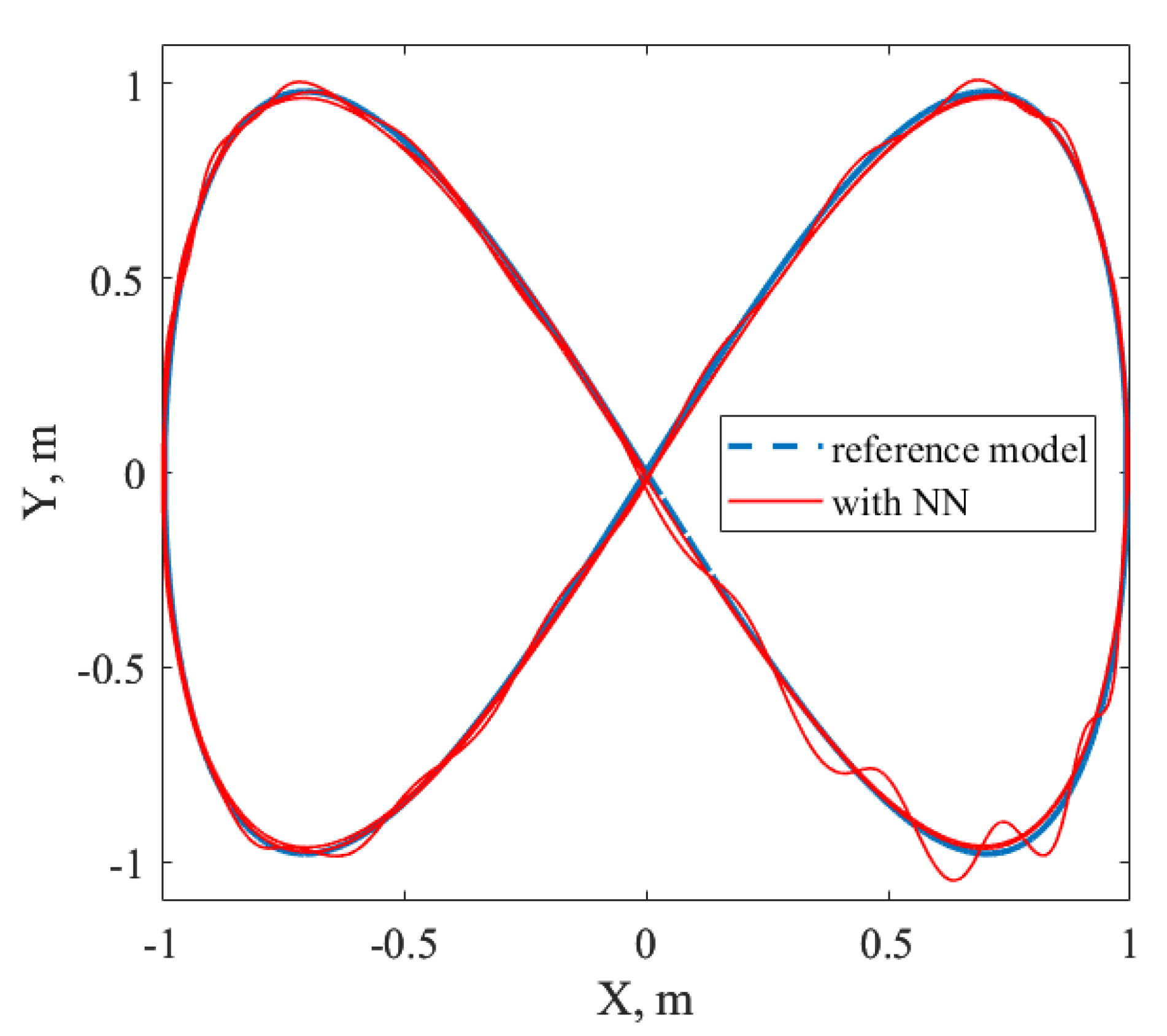
The behavior of the coordinates X and Y is shown in Figure 5. The sum of squared errors (the difference between the reference figure-eight trajectory and the real one) was reduced via the NN-compensator by $16.62\%$.

The obtained equation for $\Delta$ was used to calculate the ideal value of the parameter uncertainty for each time instant of the numerical experiment. Figure 6 illustrates that the NN-based compensator approximated such ideal $\Delta$ and verifies the theoretical result. The fact that m value was changed at 35th second did not cause the peaking phenomenon.

As the attitude control loop synthesized according to [4] also included its own NN-based compensator, Figure 7 and Figure 8 are shown to demonstrate that the parameter uncertainty of the $\psi ,\theta ,\varphi$ control loops and $J_x,J_y,J_z$ switch were approximated as well.

The same results were obtained using different values of ${\varphi }_d$. Therefore, the validity of the converter synthesis procedure for Case I was corroborated.

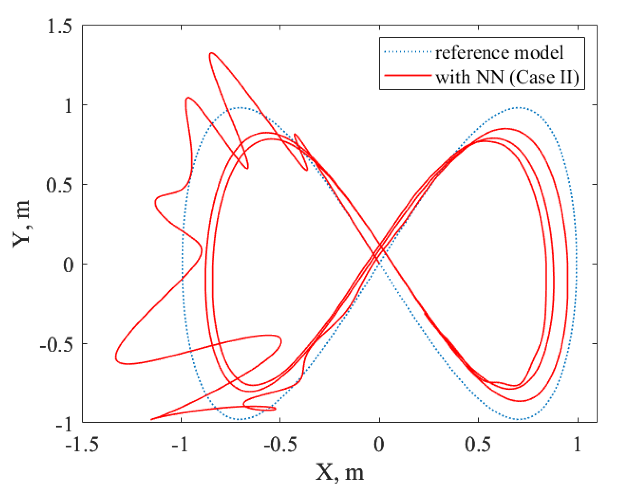
The next step was to test the adaptive control system designed for Case II. As mentioned above, the initial values of the baseline controller adjustable parameters were zeros. The results obtained for $X,Y,Z$ coordinates are shown in Figure 9 and Figure 10.

They demonstrate that the adaptive control system stabilized the quadrotor and ensured the asymptotic convergence of the tracking error to a compact set, but the steady-state error is too large for X and Y. This was mainly caused by the fact that both baseline and adaptive controllers started from zero initial conditions, which did not provide stabilization. Figures with curves to assess the quality of uncertainty approximation are not provided, as in Case II, both the NN and baseline controller have adjustable parameters and try to compensate for the whole uncertainty together.

To overcome the above-faced problems, it was decided to set the baseline controller initial conditions equal to the parameters of the characteristic polynomial of the reference model as follows: ${\widehat{k}}^x\left(0\right)=I_{3\times 3}\otimes \left[\begin{array}{cc}-25& -11\end{array}\right]$, ${\widehat{k}}^r\left(0\right)=diag(25,25,25)$. Furthermore, the experiment was conducted again. The obtained results are shown in Figure 11 and Figure 12.

Having compared the curves in Figure 4 and Figure 11 and Figure 5 and Figure 12, it was concluded that the design in Case I provided better transients quality for X, Y, and Z coordinates, so the additional adjustment of the baseline controller did not allow us to obtain any advantages. Therefore, according to the conducted experiments, Case I parameterization is a better solution to the stated problem.

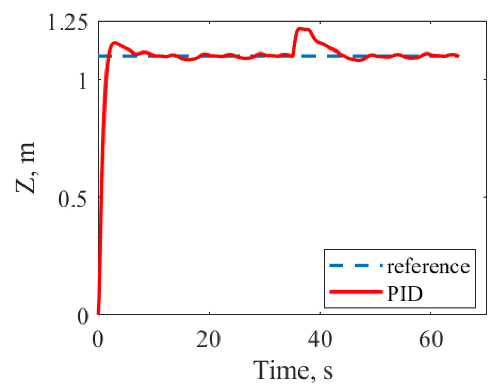
Additionally, the system on basis of the PID-controllers of altitude, attitude and position from the “ParrotMinidroneHover” project was also applied to the implemented quadrotor model. The comparison of such system with the proposed solution is considered to be fair, as we did not adjust PID-controllers by ourselves but used the best values of their parameters obtained by the developers of the “ParrotMinidroneHover” project, which were successfully applied not only for simulations but also for a real minidrone. The obtained behavior of the X, Y, and Z coordinates are shown in Figure 13 and Figure 14. It was concluded that compared to the MRAC system with NN, the PID-controllers were not capable of the parameter uncertainty compensation.

Furthermore, finally, we compared the proposed solution with the ones in which the PI/PD/PID controllers with time-invariant parameters are used as the baseline. To do so, the scheme with PID-controllers was augmented with the NN-based compensator for the X, Y, and Z coordinates. The obtained results are presented in Figure 15 and Figure 16. Comparing Figure 5, Figure 14 and Figure 16, it was concluded that the simple combination of some PID-controllers and NN-based compensators did not allow us to obtain results similar to the proposed solution. So, as in [15,16], the PID-controllers has to be adjusted via a trial and error procedure. Therefore, in [15,16], such a procedure is much more difficult, as both baseline controller parameters and adaptive controller hyperparameters have to be chosen manually. As far as the proposed solution (Case I) is concerned, the baseline controller parameters are calculated using mathematically-sound equations, and only adaptive gains and $\sigma$-modification parameters for NN are chosen via trial and error.

All in all, the obtained experimental results can be summarized as follows:

(r1)

Despite the fact that systems designed on the basis of Case I and Case II parameterizations had the same theoretical properties, the MRAC system with the NN-compesator with time-invariant baseline controller parameters allowed us to obtain better results in comparison with the adjustable baseline controller.

(r2)

The system on the basis of PID-controllers was not able to fully compensate for the parametric uncertainty.

(r3)

The simple combination of the PID-based control system with the NN-based compensator did not allow us to obtain the same results as the proposed approach. So, the baseline controller should be derived on the basis of the MRAC design procedure and have the form $k_{x}x+k_{r}r$. Moreover, as far as Case I parameterization is considered, the values of $k_x$ and $k_r$ can be directly computed.

4. Conclusions

Considering the trajectory tracking problem, the equations of the quadrotor parameter uncertainty were obtained for two cases: control signals are (i) used and (ii) not used in the parametric uncertainty parameterization. Their analysis allowed us to choose the following: (1) the neural networks to implement the compensators of Case I and Case II uncertainties and (2) the signals to form their input layers. For Case I, the adaptive laws of NN parameters were derived. For Case II, the adaptive laws of both NN and baseline controller parameters were obtained, which ensured that the augmented tracking error was UUB. The conducted experiments demonstrated that, as far as transient quality is concerned, Case I parameterization seems to be a better solution.

The main problem of the proposed solution is the above-mentioned trade-off between the value of the augmented error and the transient quality, particularly, oscillations. The scope of further research is to (i) derive a parameterization of the quadrotor to apply an identification-based adaptive control and some extension and mixing schemes to ensure some transient quality, (ii) guarantee exponential convergence instead of the assymptotic one, and (iii) consider cases when the quadrotor dynamics is affected by the wind and gravity center displacement due to load.

References

1. Glushchenko, A.; Lastochkin, K. Neural Network Based Parameter Uncertainty Compensation to Solve Quadrotor Trajectory Tracking Problem. In Proceedings of the 2022 4th International Conference on Control Systems, Mathematical Modeling, Automation and Energy Efficiency (SUMMA), Lipetsk, Russia, 9–11 November 2022; pp. 443–448. [Google Scholar]
2. Nascimento, T.P.; Saska, M. Position and attitude control of multi-rotor aerial vehicles: A survey. Annu. Rev. Control 2019, 48, 129–146. [Google Scholar] [CrossRef]
3. Fan, F.; Lin, M.; Ding, R.; Zheng, Z.; Liu, Y. Augmented-MRAC for quadrotor UAVs with parameter change. In Proceedings of the 2016 IEEE International Conference on Advanced Intelligent Mechatronics (AIM), Banff, AB, Canada, 12–15 July 2016; pp. 501–506. [Google Scholar]
4. Glushchenko, A.; Lastochkin, K. Neural Network-based Direct Model Reference Adaptive Control of Quadrotor Attitude. In Proceedings of the 2022 16th International Conference on Stability and Oscillations of Nonlinear Control Systems (Pyatnitskiy’s Conference), Moscow, Russia, 1–3 June 2022; pp. 1–4. [Google Scholar]
5. Liu, C.; Pan, J.; Chang, Y. PID and LQR trajectory tracking control for an unmanned quadrotor helicopter: Experimental studies. In Proceedings of the 2016 35th Chinese Control Conference (CCC), Chengdu, China, 27–29 July 2016; pp. 10845–10850. [Google Scholar]
6. Voos, H. Nonlinear state-dependent Riccati equation control of a quadrotor UAV. In Proceedings of the 2006 IEEE International Conference on Control Applications, Munich, Germany, 4–6 October 2006; pp. 2547–2552. [Google Scholar]
7. Madani, T.; Benallegue, A. Control of a quadrotor mini-helicopter via full state backstepping technique. In Proceedings of the 45th IEEE Conference on Decision and Control, San Diego, CA, USA, 13–15 December 2006; pp. 1515–1520. [Google Scholar]
8. Altug, E.; Ostrowski, J.P.; Taylor, C.J. Control of a quadrotor helicopter using dual camera visual feedback. Int. J. Robot. Res. 2005, 24, 329–341. [Google Scholar] [CrossRef]
9. Zhang, Y.; Chen, Z.; Zhang, X.; Sun, Q.; Sun, M. A novel control scheme for quadrotor UAV based upon active disturbance rejection control. Aerosp. Sci. Technol. 2018, 79, 601–609. [Google Scholar] [CrossRef]
10. Abdul Ghaffar, A.F.; Richardson, T.S. Position tracking of an underactuated quadrotor using model reference adaptive control. In Proceedings of the AIAA Guidance, Navigation, and Control Conference, AIAA SciTech, San Diego, CA, USA, 4–8 January 2016; pp. 1–13. [Google Scholar]
11. Jin, X.Z.; He, T.; Wu, X.M.; Wang, H.; Chi, J. Robust adaptive neural network-based compensation control of a class of quadrotor aircrafts. J. Frankl. Inst. 2020, 357, 12241–12263. [Google Scholar] [CrossRef]
12. Dierks, T.; Jagannathan, S. Output feedback control of a quadrotor UAV using neural networks. IEEE Trans. Neural Netw. 2010, 21, 50–66. [Google Scholar] [CrossRef] [PubMed]
13. Wang, M.; Chen, B.; Lin, C. Fixed-time Backstepping control of quadrotor trajectory tracking based on neural network. IEEE Access 2020, 8, 177092–177099. [Google Scholar] [CrossRef]
14. Barron, A.R. Universal approximation bounds for superpositions of a sigmoidal function. IEEE Trans. Inf. Theory 1993, 39, 930–945. [Google Scholar] [CrossRef]
15. Lopez-Sanchez, I.; Perez-Alcocer, R.; Moreno-Valenzuela, J. Trajectory tracking double two-loop adaptive neural network control for a Quadrotor. J. Frankl. Inst. 2023, 360, 3770–3799. [Google Scholar] [CrossRef]
16. Doukhi, O.; Lee, D.J. Neural network-based robust adaptive certainty equivalent controller for quadrotor UAV with unknown disturbances. Int. J. Control Autom. Syst. 2019, 17, 2365–2374. [Google Scholar] [CrossRef]
17. Choutri, K.; Lagha, M.; Dala, L.; Lipatov, M. Quadrotors trajectory tracking using a differential flatness-quaternion based approach. In Proceedings of the 2017 7th International Conference on Modeling, Simulation, and Applied Optimization (ICMSAO), Sharjah, United Arab Emirates, 4–6 April 2017; pp. 1–5. [Google Scholar]
18. Funahashi, K.; Nakamura, Y. Approximation of Dynamical Systems by Continuous Time Recurrent Neural Networks. Neural Netw. 1993, 6, 801–806. [Google Scholar] [CrossRef]
19. Nguyen, N.T. Model-Reference Adaptive Control—A Primer; Springer International Publishing: London, UK, 2018. [Google Scholar]
20. Na, J.; Herrmann, G.; Zhang, K. Improving transient performance of adaptive control via a modified reference model and novel adaptation. Int. J. Robust Nonlinear Control 2017, 27, 1351–1372. [Google Scholar] [CrossRef]
Figure 1. Schematic representation of quadrotor.
Computation 11 00163 g001
Figure 2. Block scheme of quadrotor control system.
Computation 11 00163 g002
Figure 3. Neural network structure.
Computation 11 00163 g003
Figure 4. Transients of Z for control systems with (Case I) and without NN-based compensator.
Computation 11 00163 g004
Figure 5. Transients of X and Y for control systems with (Case I) and without NN-based compensator.
Computation 11 00163 g005
Figure 6. Approximation of the ideal parameter uncertainty in neural network for X , Y , Z .
Computation 11 00163 g006
Figure 7. Approximation of the ideal parameter uncertainty by neural network for ψ , θ , ϕ .
Computation 11 00163 g007
Figure 8. The behavior of ψ , θ , ϕ for MRAC system with NN.
Computation 11 00163 g008
Figure 9. Transients of Z coordinate for control system with NN-based compensator for Case II using baseline controller with zero initial conditions.
Computation 11 00163 g009
Figure 10. Transients of X and Y coordinates for control system with NN-based compensator for Case II using baseline controller with zero initial conditions.
Computation 11 00163 g010
Figure 11. Transients of Z coordinate for control system with NN-based compensator for Case II using baseline controller with non-zero initial conditions.
Computation 11 00163 g011
Figure 12. Transients of X and Y coordinates for control system with NN-based compensator for Case II using baseline controller with non-zero initial conditions.
Computation 11 00163 g012
Figure 13. Transients of Z coordinate for PID-based control system.
Computation 11 00163 g013
Figure 14. Transients of X and Y coordinates for PID-based control system.
Computation 11 00163 g014
Figure 15. Transients of Z coordinate for PID+NN control system.
Computation 11 00163 g015
Figure 16. Transients of X and Y coordinates for PID+NN control system.
Computation 11 00163 g016
Disclaimer/Publisher’s Note: The statements, opinions and data contained in all publications are solely those of the individual author(s) and contributor(s) and not of MDPI and/or the editor(s). MDPI and/or the editor(s) disclaim responsibility for any injury to people or property resulting from any ideas, methods, instructions or products referred to in the content.