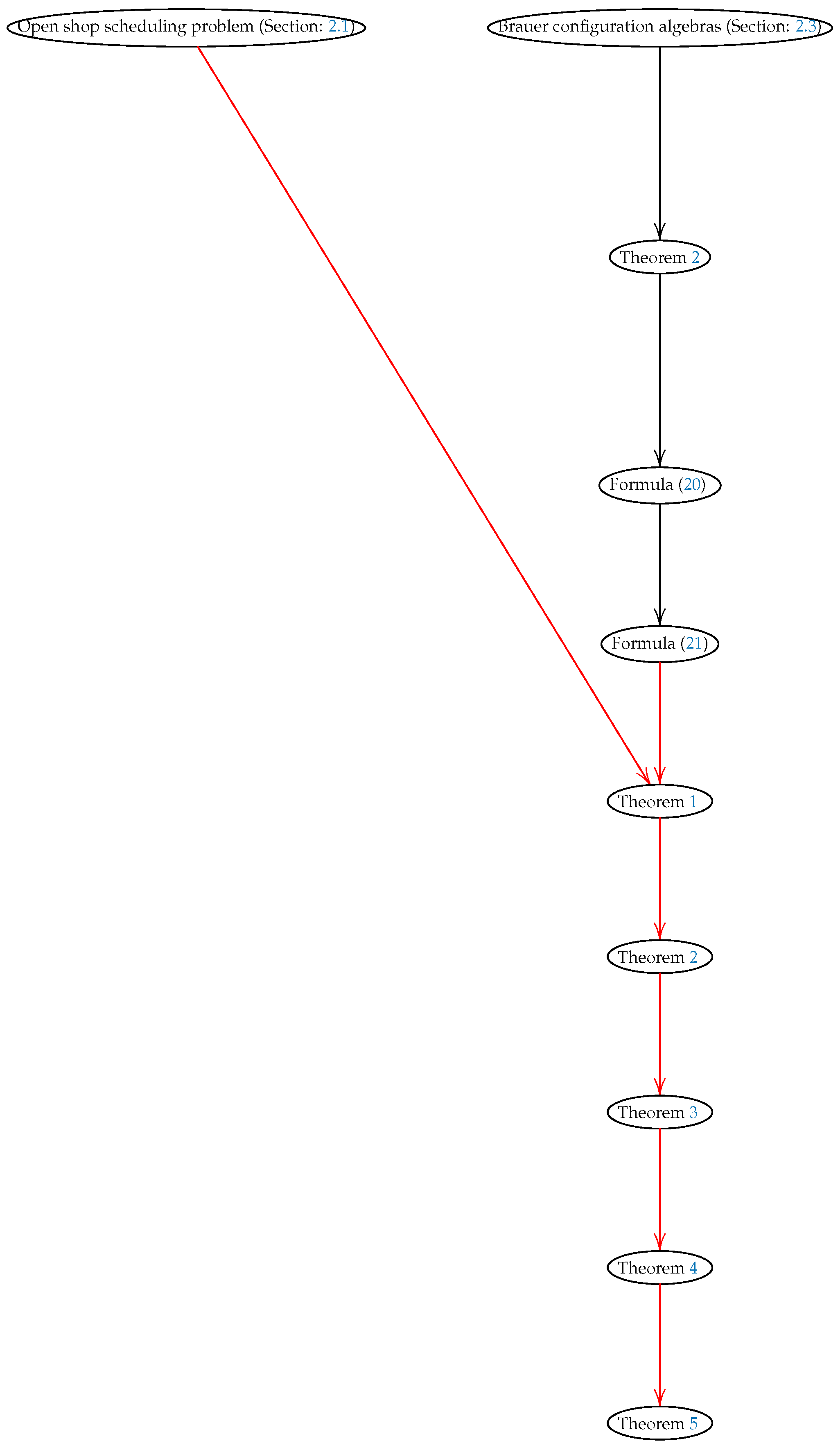
2.1. The Open Shop Scheduling Problem
An instance of the OSSP consists of m machines, and n jobs, . Each job consists of m independent operations, , with , the operation of job has to be processed on machine , which takes uninterrupted time units. For every job, the order in which its operations have to be processed does not matter. In fact, different jobs may receive different processing orders.
No job is simultaneously processed by two different machines. The optimal makespan is usually denoted by
. The overall processing time assigned to a machine
is called the
load of the machine, denoted
[
4,
5].
The maximum job processing time is denoted and the maximum machine load is denoted .
Since no job can be simultaneously processed by two machines, it holds that and . Thus, . It is worth noting that there is always a schedule whose makespan equals the lower bound .
For a schedule associated with an OSSP with m machines and n different jobs, the corresponding processing time matrix (PTM), , is defined. In such a case, the overall processing time of the work matrix is given by the sum .
We let () denote the release time (due date) associated with a job J, where is the strict due date.
An objective of some OSSP problems is to minimize the value with certain constraints. For instance:
We recall that the idle time is a period of time in which a machine, M, is ready and available but is not doing anything productive. Let denote the idle time associated with all the machines, , of a schedule. The waiting time for job is denoted , whereas denotes the total waiting time associated with jobs of a schedule.
By way of example, the following is a PTM with three machines,
, and
, and two jobs,
and
, for which
.
For each PTM P, it is possible to define its cumulative matrix (CPTM) whose entries give the time that the jth machine takes to process the ith job. () is associated with waiting time (idle time).
The overall joint processing time (OJPT)
is given by the following:
The cumulative matrix of the matrix (
2) (whose entries have been organized according to the processing time, i.e.,
) is
If is an -PTM then the matrix with , is an element of the symmetry group and . We let () denote the idle time (waiting time) associated with configuration .
Calderon [
36] proposed the minimum bound for a fixed configuration
encoding an OSSP as
where
,
,
,
n is the number of jobs.
For example, the configuration
optimizes
for the PTM
P given in (
2) provided that
In this case,
, ,
,
,
,
,
,
.
Calderon [
36] observed that
of the matrices that end the process without interruptions have a
value bounded by
. In such a case we say that the PMT satisfies the
condition. If the configuration
satisfies the
condition then we write
. Matrices obtained via column permutations of the cumulative matrix associated with a PTM are said to be
configurations. We let
denote the set of all configurations. Thus, an optimal configuration (giving an optimal
) arises from the configuration space with
elements.
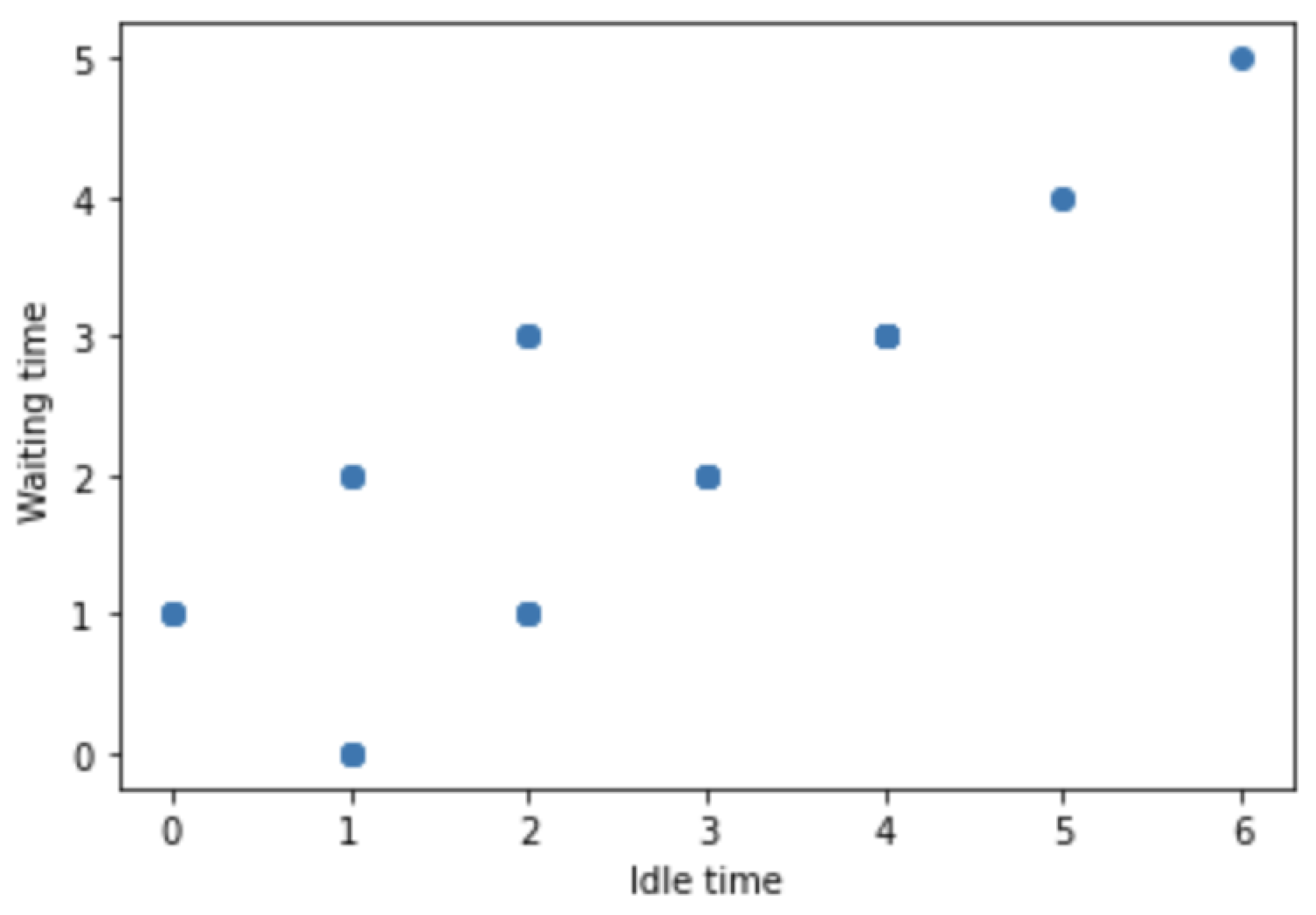
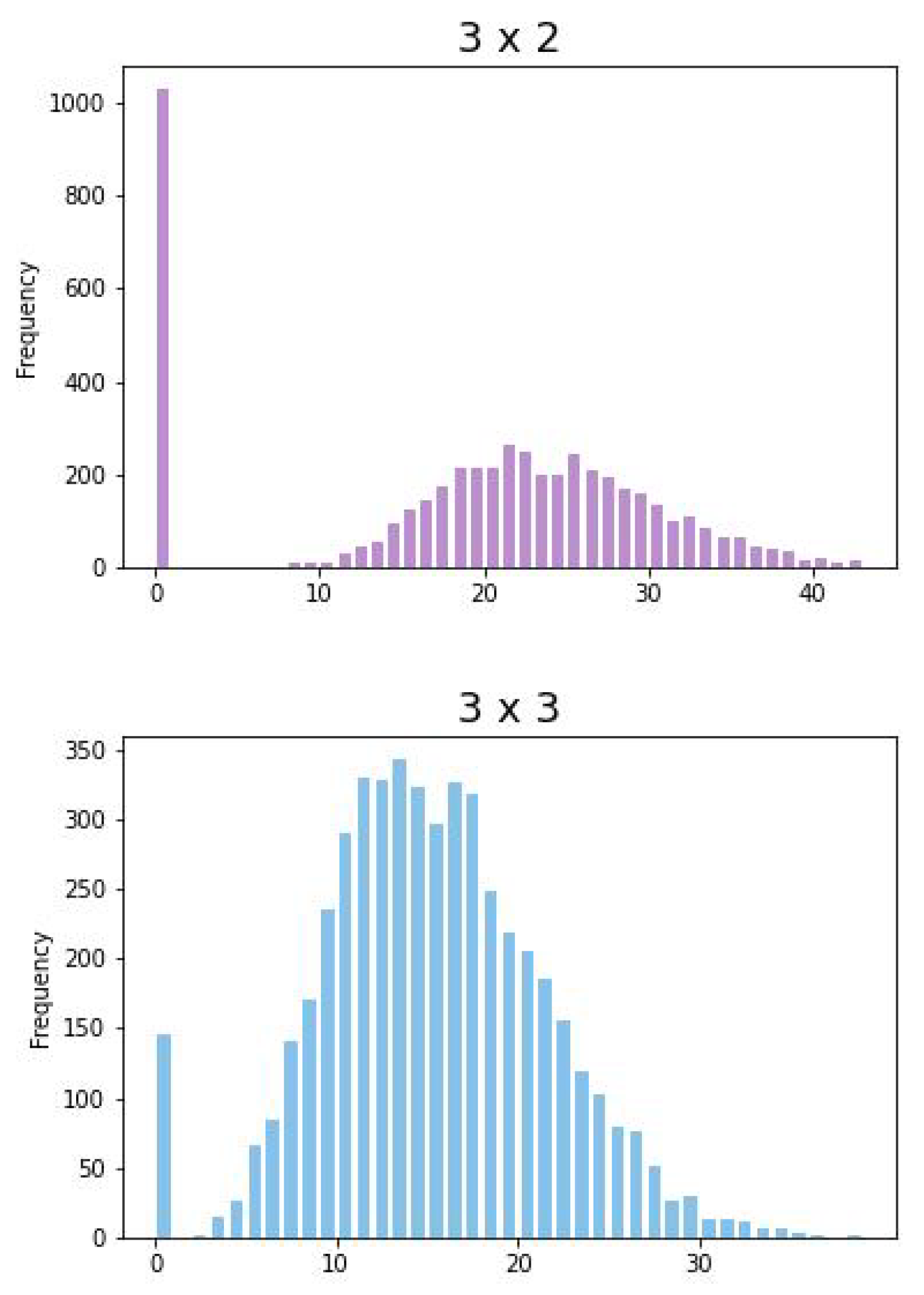
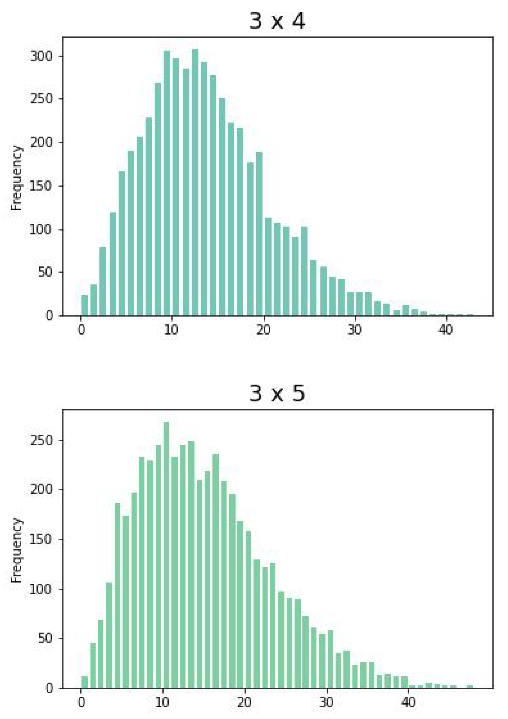
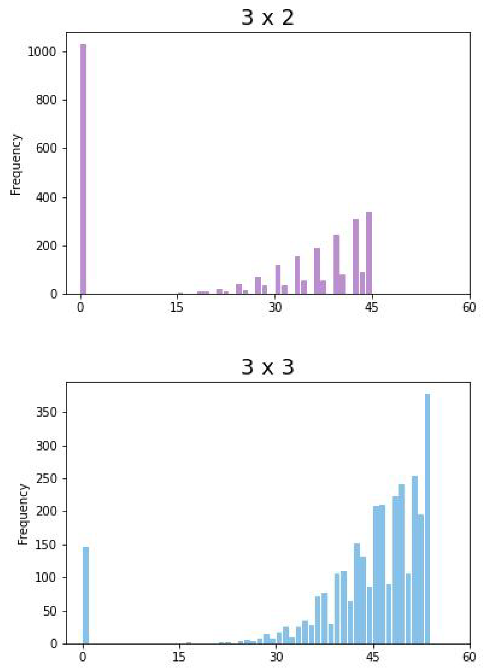
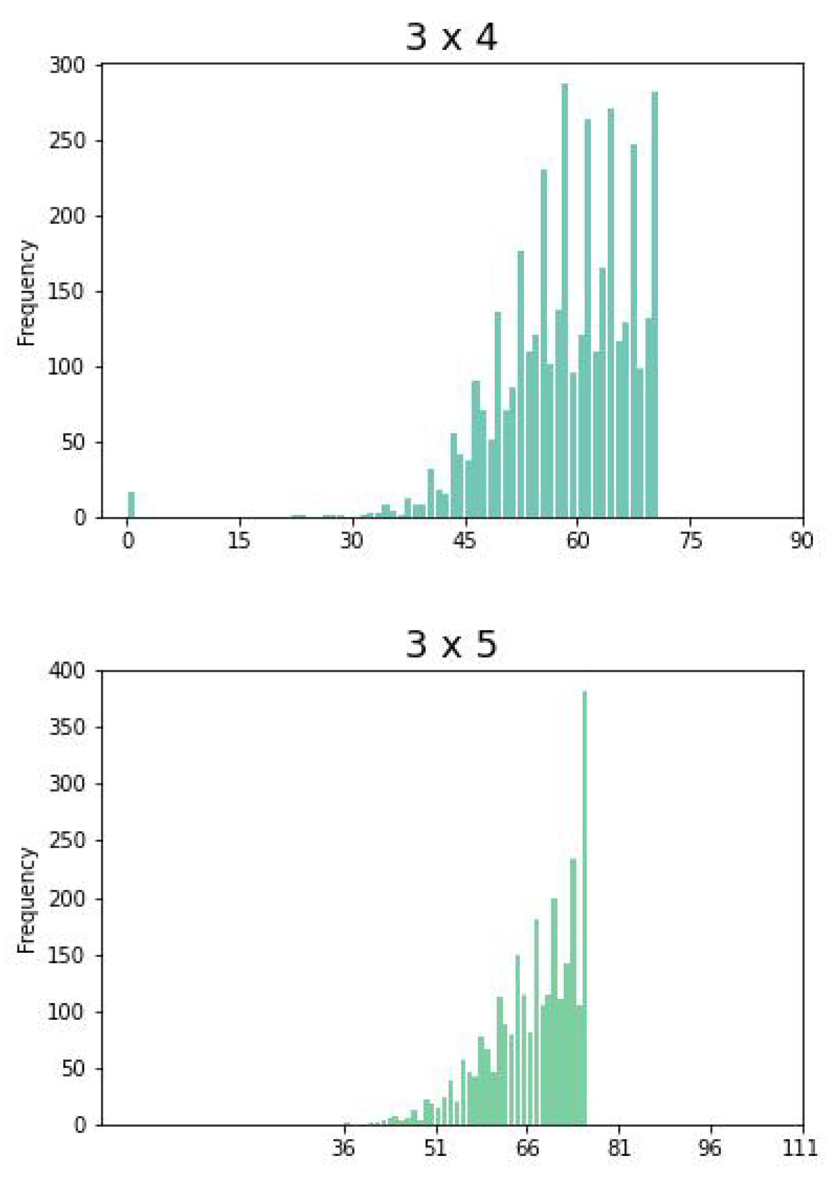
Figure 2 shows idle and waiting times of all different configurations given by the CPTM (
6). Note that, the bound
is given by the points
and
. In general,
is given by points on a
optimal line of the form
.
2.2. Path Algebras
This section presents some definitions and notation regarding path algebras.
A quiver, Q, is a quadruple of the form , where is a set of vertices, is a set of arrows, and are maps that assign the starting vertex (ending vertex) () of an arrow . For instance, the arrow denoted in the form has a starting vertex and an ending vertex .
A path of length with source and target (or more briefly, from to ) is a sequence where for all , and . We let denote such a path. In particular, each point, , has an associated stationary path, , of length 0.
If X is a set of paths in quiver Q then , where denotes the length of the path x (i.e., the number of arrows contained in x). We let () denote the length of path P (the set of all paths P for which ).
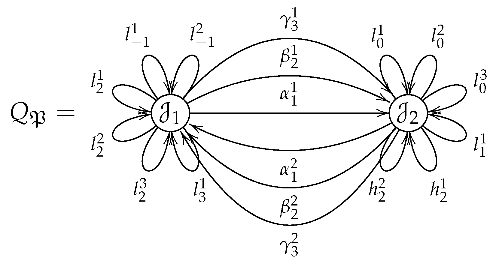
Figure 3 shows an example of a quiver,
Q, with three vertices,
, and
, and three arrows,
, and
.
If
is an algebraically closed field then the
path algebra of
Q is the
-algebra whose underlying
-vector space has as its basis the set of all paths of length
in
Q, such that the product of two basis vectors is given by the usual concatenation of paths. Note that in general, path algebras are noncommutative. Let
denote the
center of a path algebra (
if and only if
, for all
). For instance,
(where
is a complete set of primitive orthogonal idempotents) is a basis of the algebra
, where
Q is the quiver given in
Figure 3, and
.
Let Q be a finite and connected quiver. The two-sided ideal, , of the path algebra generated (as an ideal) by the arrows of Q is called the arrow ideal of . A two-sided ideal, I, of is said to be admissible if there exists such that .
If I is an admissible ideal of , the pair is said to be a bound quiver. The quotient algebra is said to be the algebra of the bound quiver or, simply, a bound quiver algebra.
Let
Q be a quiver. A
relation in
Q with coefficients in
is an
-linear combination of paths of at least 2 in length, and having the same source and target. Thus, a relation
is an element of
such that
where the
are scalars (not all zero) and the
are paths in
Q of length at least 2 such that, if
, then the source (or the target, respectively) of
coincides with that of
.
If , the preceding relation is called a zero relation or a monomial relation. If it is of the form (where and are two paths), it is called a commutativity relation.
If
is a set of relations for a quiver
Q such that the ideal they generate
is admissible, we say that the quiver
Q is bound by the relation
or by the relations
[
29,
30].
Henceforth, we let denote the radical of a path algebra , which is the intersection of all maximal ideals. In fact, if I is an admissible ideal of , it holds that .
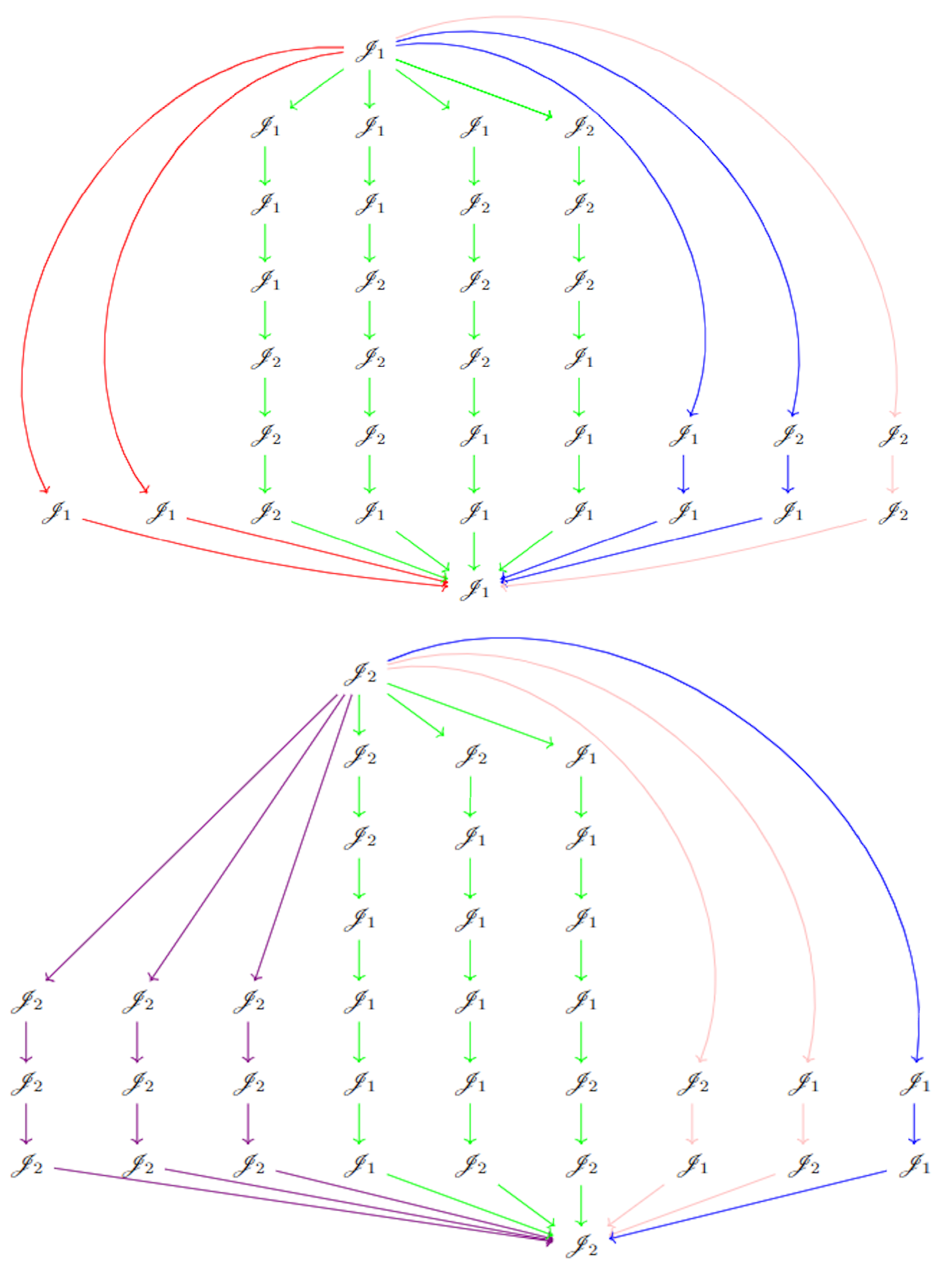
A module, M, over a bound quiver algebra is said to be decomposable, if there are nonzero modules and such that . Otherwise, M is said to be indecomposable.
Each vertex x in quiver Q has an associated indecomposable projective module, , over a bound quiver algebra, , generated by all the paths in Q with x as its starting point. In particular, .
As an example,
is an admissible ideal of the algebra
defined by the quiver shown in
Figure 3. The algebra
is generated by the basis
. Thus,
.
2.3. Multisets and Brauer Configuration Algebras
A
multiset is an ordered pair
where
M is a set and
f is a function from
M to the nonnegative integers; for each
,
is said to be the
multiplicity of
m [
37].
If
M is a finite set, say
, then a multiset
can be written as a word with the form described by identity (
9).
Multisets are helpful tools in the theory of partitions, where they are used to obtain formulas for restricted partitions via inversions.
If
and
are multisets then
The
message associated with a collection of multisets
is given by the usual word concatenation defined by the Formula (
12)
where for
h fixed, the word
is given by the identity (
13)
If an element
then its
valency denoted
is given by the Formula (
14) [
29,
31].
Green and Schroll [
29] defined
Brauer configurations which are oriented systems of multisets with the form
where
is a multiplicity map
such that
, with
, we let
denote the product
. Henceforth, if no confusion arises, we will omit the symbol
to denote a multiset
associated with a Brauer configuration
.
Elements
(multisets
) were named
vertices (
polygons) by Green and Schroll [
29]. If
is such that
(
) then the vertex
is said to be
truncated (
non-truncated). A Brauer configuration is
reduced if it has not truncated vertices.
In the theory of Brauer configuration algebras, the collection
of all polygons containing a fixed vertex
is endowed with a linear order <. Thus, there is a minimum
polygon and a maximum polygon
. In such a case, it holds that
where
denotes the
ith copy of
.
A chain (
17) is a
successor sequence associated with the vertex
.
An
orientation of a Brauer configuration is obtained by adding to each successor sequence a new relation
. Thus, it is obtained a circular ordering, which define equivalent orderings of the form
Remark 1. Henceforth, we assume that relations between the same polygons in different circular orderings are the same [31]. If
, and
are Brauer configurations then the Brauer configuration
such that
,
is said to be disconnected, otherwise is connected.
Brauer Configuration Algebras
Green and Schroll [
29] named Brauer configuration algebras to those bound quiver algebras of type
defined by a Brauer configuration
(see Remark 1). In such a case the polygons in
give the set of vertices
of the quiver
, whereas its arrows are defined by coverings in completed successor sequences [
29,
30,
31].
is bounded by relations of the following types:
Identification of special cycles defined by vertices in the same polygon.
Multiplication of each special cycle by its first arrow.
If it exists, multiplication of arrows in different special cycles.
Henceforth, we will assume the notations Q, I, and for quivers, admissible ideals and Brauer configuration algebras defined by a fixed Brauer configuration .
Remark 2. Green and Schroll [29] proved that Brauer configuration algebras are indecomposable as algebras if the corresponding Brauer configurations are connected. Furthermore, they are multiserial and symmetric. Particularly, they established that the underlying Brauer configuration’s nontruncated vertices give the indecomposable projective modules structure over a Brauer configuration algebra. For instance, the number of such vertices in a fixed polygon gives the number of summands in the radical and heart of the corresponding indecomposable projective module. They also introduced the formula (20) for the dimension of a Brauer configuration algebra induced by a Brauer configuration with polygons.
where
denotes the
jth triangular number and
(see (
15)).
The following is an interpretation of the formula introduced by Sierra [
35] to obtain the dimension of the center of a Brauer configuration algebra
.
where
.


 ,
, 


