Pricing and Hedging Index Options under Mean-Variance Criteria in Incomplete Markets

Abstract

This paper studies the portfolio selection problem where tradable assets are a bank account, and standard put and call options are written on the S&P 500 index in incomplete markets in which there exist bid–ask spreads and finite liquidity. The problem is mathematically formulated as an optimization problem where the variance of the portfolio is perceived as a risk. The task is to find the portfolio which has a satisfactory return but has the minimum variance. The underlying is modeled by a variance gamma process which can explain the extreme price movement of the asset. We also study how the optimized portfolio changes subject to a user’s views of the future asset price. Moreover, the optimization model is extended for asset pricing and hedging. To illustrate the technique, we compute indifference prices for buying and selling six options namely a European call option, a quadratic option, a sine option, a butterfly spread option, a digital option, and a log option, and propose the hedging portfolios, which are the portfolios one needs to hold to minimize risk from selling or buying such options, for all the options. The sensitivity of the price from modeling parameters is also investigated. Our hedging strategies are decent with the symmetry property of the kernel density estimation of the portfolio payout. The payouts of the hedging portfolios are very close to those of the bought or sold options. The results shown in this study are just illustrations of the techniques. The approach can also be used for other derivatives products with known payoffs in other financial markets.

1. Introduction

Financial risk and liability can be mitigated through appropriately trading in financial markets. In other words, having a liability, which is normally stochastic, a user would want to reduce their risk by buying or selling some other financial instruments available in the markets [1,2,3]. In complete markets, where all assets are perfectly liquid and there is no transaction cost, it has been shown by Black and Scholes [4] that financial derivatives can be uniquely priced and perfectly hedged by dynamically trading their underlying and cash. However, this is not true in incomplete markets, in which liquidity is limited. Moreover, the pricing and hedging problems, in practice, are highly subjective. Different agents may hold different current financial positions, view risk differently, and have different views on the future values of the assets, see e.g., [5,6,7,8,9].

Most works in pricing and hedging financial derivatives assume market completeness. Following the ground-breaking work by Black and Scholes [4], there has been extensive literature on derivative pricing based on a risk-neutral measure. The fair price of a derivative is determined by the expectation of the discounted terminal payoff of the derivative under a risk-neutral measure. The price, in terms of the expectation, can be easily and analytically derived if its density is known, see [10,11,12]. For those where the density is unknown, the no-arbitrage price can be computed by solving the corresponding partial differential equation derived from the Feynman–Kac representation [13,14,15]. For example, Sepp [16] derived analytical pricing formulas for options on realized variance under Heston stochastic volatility model, whereas the pricing formulas for an interest rate swap under the extended Cox–Ingersoll–Ross (ECIR) and the constant elasticity of variance processes were proposed in [17,18,19,20,21].

In incomplete markets, the classic risk-neutral approach cannot be applied. Most works derive formulas for indifference prices by using convex duality theory, see e.g., [22,23,24]. However, the scheme is complex and hard to apply in practice. A more practical approach for option pricing was proposed by Breeden and Litzenberger [25]. The option payoff is replicated by the collection of other options with different strikes finitely available in the markets. The price of the payoff is thus the cost of replication. Although the approach works reasonably well in practice when there are enough options available in the markets, the combination of replicating the payoff might not be most suitable. Moreover, the subjective factors, which are different for each individual, are not taken into account. Thus, a more efficient scheme of pricing called “indifference pricing” was proposed. An indifference price is a price a seller (buyer) needs to take (can pay) so that the risk after selling or buying is not worsened, see [6,26]. In contrast to the approaches mentioned above, indifference pricing takes subjectivity into account. The selling and buying prices of financial derivatives for different agents can be different. Moreover, the approach ensures that the combination for derivatives hedging is the best available in the markets. The indifference pricing approach is built on an optimal investment model. Armstrong et al. [27] illustrated the use of the indifference pricing technique to price and hedge index options written on the S&P 500 index under the exponential loss utility by numerically directly solving the primal problem. Another recent work that focused on indifference pricing and hedging by solving the primal problem was by Pennanen and Bonatto [28]. They computed hedging portfolios in oil markets under the exponential loss utility. As opposed to the exponential loss utility, there are various risk measures such as the mean-variance criteria, the value-at-risk (VaR), and the conditional value-at-risk (CVaR). Although the portfolio optimization models of such risk measures have been extensively studied, see [29,30,31,32], the study of indifference prices and hedging, in practice, is still limited.

In this paper, we consider indifference pricing and hedging where risk is measured by a portfolio’s return variance, and the quotes come with bid–ask prices as well as the sizes, and the maximum quantities one can buy or sell. In other words, our portfolio optimization model in which the indifference pricing and hedging are built upon an extension of the mean-variance portfolio optimization, first proposed by Markowitz [33], where we have bid–ask prices and illiquidity. As an example, the technique is illustrated in the mini S&P 500 index options market. The trading assets are a bank account with zero interest rate, and the mini put and call options written on the S&P 500 index. The case where the interest rate is not zero can be done in the same manner. The underlying is modeled by a variance-gamma process (see [26,34]), which is similar to the Geometric Brownian motion except that the time change is gamma distributed. This lets the process have control over skewness and kurtosis which is more realistic as it is known that a return in stock markets usually has fat tails.

Given a required average return, we first determine the optimal portfolio and plot its payout as a function of the index value at maturity. We also numerically illustrate the effects of various parameters including modeling parameters and the required return and plot the efficient frontier of the portfolio. Next, we compute indifference prices for buying and selling six different options namely a call option, a quadratic option, a log option, a digital option, a butterfly spread option, and a sine option. The hedging portfolio, the portfolio one needs to hold after selling or buying in order to mitigate risk, for each option is also computed. We showed that all options are hedged reasonably well given the quantity constraints and spreads. The technique can be applied to any other markets for any European options whose payouts are functions of the underlying at maturity.

2. Methodology

2.1. Data

The tradable assets are a bank account with zero interest rate, and 199 mini S&P 500 put and call options with different strikes.

Table 1. Taken from Bloomberg terminal on the 19 May 2020 at 12:00:01 Bangkok time.

Bloomberg Ticker	Bid Price	Ask Price	Bid Size	Ask Size
S&P 19/05/2020 C262 Equity	34.54	35.09	10	10
S&P 19/05/2020 P262 Equity	1.93	2.01	7	26
S&P 19/05/2020 C263 Equity	33.63	34.18	10	10
S&P 19/05/2020 P263 Equity	2.02	2.10	12	5

shows an example of mini S&P 500 option prices taken on 19 May 2020 at 12:00:01 New York time. The spot is 295.42. The investment horizon is one month which is exactly the time when all of the options expire. One can see that the options come with finite liquidities. For example, if a trader wants to buy a call option with strike 262 (the first row), there are only 10 contracts available. Although we have 199 options, it is worth noting that there is only one random factor which is the value of the index at maturity as all of the options are written on the same index. The full details on all 199 options can be found in

Table A1. Taken from Bloomberg terminal on the 19 May 2020 at 12:00:01 Bangkok time.

A	B	C	D	E	F	A	B	C	D	E	F
Strike	Bid	Ask	IsPut	Bid Size	Ask Size	Strike	Bid	Ask	IsPut	Bid Size	Ask Size
265	31.84	32.36	0	10	10	322	0.43	0.48	0	19	10
270	27.42	27.9	0	10	10	323	0.39	0.43	0	9	17
275	23.14	23.56	0	10	10	325	0.31	0.35	0	6	16
278	20.65	21.04	0	10	10	327	0.25	0.28	0	5	13
279	19.9	20.1	0	1	1	328	0.22	0.26	0	14	20
280	19.08	19.29	0	1	1	330	0.18	0.21	0	5	19
281	18.28	18.5	0	1	1	335	0.11	0.14	0	1	3
282	17.49	17.68	0	16	16	340	0.06	0.1	0	1	1
283	16.71	16.9	0	32	32	345	0.01	0.07	0	1050	1
284	15.92	16.12	0	48	48	350	0.02	0.05	0	1	1
285	15.16	15.37	0	48	48	250	1.12	1.17	1	16	10
286	14.41	14.59	0	64	64	255	1.4	1.48	1	15	210
287	13.67	13.85	0	80	80	260	1.76	1.84	1	8	134
288	12.93	13.11	0	80	80	264	2.11	2.2	1	13	108
289	12.22	12.39	0	96	96	266	2.32	2.4	1	6	2
290	11.51	11.69	0	96	96	267	2.42	2.51	1	6	5
291	10.82	11	0	112	112	268	2.54	2.62	1	2	14
292	10.14	10.34	0	162	112	269	2.65	2.74	1	4	106
293	9.49	9.68	0	162	112	271	2.9	2.99	1	1	107
294	8.85	9.04	0	50	128	272	3.02	3.13	1	2	100
295	8.24	8.42	0	50	128	273	3.16	3.27	1	2	101
296	7.65	7.82	0	50	128	274	3.29	3.41	1	100	101
297	7.07	7.25	0	50	128	276	3.61	3.72	1	1	100
298	6.52	6.69	0	50	128	277	3.77	3.89	1	1	100
299	6	6.16	0	50	128	307	14.8	15.08	1	1	1
300	5.5	5.65	0	50	144	308	15.4	15.84	1	10	10
301	5.02	5.16	0	50	144	309	16.12	16.58	1	10	10
302	4.57	4.71	0	50	160	311	17.64	18.14	1	10	10
303	4.14	4.28	0	50	176	312	18.43	18.95	1	10	10
304	3.74	3.88	0	50	192	313	19.24	19.78	1	10	10
305	3.37	3.5	0	100	308	314	20.07	20.63	1	10	10
306	3.03	3.15	0	100	324	316	21.78	22.39	1	10	10
310	1.91	2	0	110	1	317	22.66	23.29	1	10	10
315	1.02	1.1	0	5	9	318	23.56	24.2	1	10	10
320	0.55	0.6	0	7	11	319	24.47	25.12	1	10	10
265	2.21	2.29	1	9	2	321	26.32	27	1	10	10
270	2.77	2.86	1	4	4	322	27.25	27.95	1	10	10
275	3.45	3.56	1	2	100	323	28.2	28.9	1	10	10
278	3.94	4.06	1	1	100	325	30.11	30.83	1	10	10
279	4.1	4.24	1	100	100	327	32.04	32.77	1	10	10
280	4.29	4.43	1	100	100	328	33.01	33.75	1	10	10
281	4.47	4.62	1	50	50	330	34.96	35.71	1	10	10
282	4.68	4.83	1	50	50	335	39.88	40.65	1	10	10
283	4.89	5.04	1	50	50	340	44.83	45.61	1	10	10
284	5.11	5.27	1	50	50	345	49.8	50.58	1	10	10
285	5.34	5.5	1	50	50	350	54.78	55.57	1	10	10
286	5.58	5.75	1	50	50	329	0.2	0.23	0	6	18
287	5.83	6.01	1	50	50	329	33.99	34.73	1	10	10
288	6.1	6.28	1	50	50	331	0.16	0.2	0	16	24
289	6.37	6.57	1	50	50	332	0.15	0.18	0	6	18
290	6.72	6.86	1	144	50	331	35.94	36.7	1	10	10
291	6.97	7.18	1	50	50	332	36.92	37.68	1	10	10
292	7.3	7.51	1	50	50	333	0.13	0.17	0	19	28
293	7.7	7.86	1	128	50	333	37.91	38.67	1	10	10
294	7.99	8.23	1	50	50	334	0.12	0.15	0	1	6
295	8.37	8.61	1	50	50	334	38.89	39.66	1	10	10
296	8.77	9.02	1	50	50	336	0.1	0.13	0	1	3
297	9.18	9.44	1	142	13	336	40.87	41.64	1	10	10
298	9.62	9.9	1	13	13	337	0.09	0.12	0	1	12
299	10.09	10.37	1	125	13	338	0.08	0.11	0	6	17
300	10.59	10.87	1	112	13	337	41.86	42.63	1	10	10
301	11.11	11.4	1	96	109	338	42.85	43.62	1	10	10
302	11.65	11.94	1	80	80	339	0.07	0.11	0	18	12
303	12.22	12.52	1	64	64	341	0.03	0.11	0	1050	950
304	12.8	13.13	1	48	48	339	43.84	44.61	1	10	10
305	13.46	13.74	1	32	32	341	45.83	46.6	1	10	10
306	14.11	14.4	1	16	16	342	0.02	0.11	0	1250	1050
310	16.87	17.35	1	10	10	342	46.82	47.6	1	10	10
315	20.92	21.5	1	10	10	343	0.02	0.1	0	950	950
320	25.39	26.06	1	10	10	344	0.04	0.1	0	1	900
324	0.34	0.39	0	14	25	343	47.81	48.59	1	10	10
324	29.15	29.87	1	10	10	344	48.81	49.59	1	10	10
326	0.28	0.31	0	6	11	346	0.03	0.09	0	1	950
326	31.07	31.8	1	10	10	346	50.8	51.58	1	10	10
250	45.66	46.3	0	10	10	347	51.8	52.58	1	10	10
255	40.96	41.57	0	10	10	348	52.79	53.57	1	10	10
260	36.36	36.93	0	10	10	349	53.79	54.57	1	10	10
264	32.73	33.27	0	10	10	262	34.54	35.09	0	10	10
266	30.95	31.46	0	10	10	263	33.63	34.18	0	10	10
267	30.06	30.56	0	10	10	262	1.93	2.01	1	7	26
268	29.18	29.67	0	10	10	263	2.02	2.1	1	12	5
269	28.3	28.78	0	10	10	251	44.71	45.35	0	10	10
271	26.56	27.02	0	10	10	252	43.77	44.4	0	10	10
272	25.7	26.15	0	10	10	253	42.83	43.45	0	10	10
273	24.84	25.28	0	10	10	254	41.9	42.51	0	10	10
274	23.99	24.42	0	10	10	256	40.03	40.63	0	10	10
276	22.31	22.71	0	10	10	257	39.11	39.7	0	10	10
277	21.48	21.87	0	10	10	258	38.2	38.78	0	10	10
307	2.71	2.83	0	100	340	259	37.28	37.86	0	10	10
308	2.42	2.53	0	101	356	261	35.45	36.01	0	10	10
309	2.15	2.25	0	102	1	251	1.17	1.22	1	15	8
311	1.69	1.78	0	113	1	252	1.23	1.28	1	12	12
312	1.49	1.58	0	102	4	253	1.29	1.34	1	3	16
313	1.32	1.4	0	3	2	254	1.35	1.4	1	14	4
314	1.16	1.24	0	4	8	256	1.46	1.54	1	21	13
316	0.91	0.96	0	2	1	257	1.53	1.61	1	23	13
317	0.8	0.85	0	2	6	258	1.6	1.68	1	19	12
318	0.71	0.76	0	3	9	259	1.68	1.76	1	14	9
319	0.63	0.67	0	5	4	261	1.84	1.92	1	12	9
321	0.49	0.54	0	7	16

in Appendix A.

2.2. Portfolio Optimization

In this section, we introduce the asset-liability management model where bid and ask spreads as well as limited quantities for buying and selling are present. The model is an extension of the classical portfolio optimization model described in [33] where an agent may have an initial liability and expects to reduce the risk associated with the terminal loss. The detailed process of the optimization as well as its algorithms are also provided here.

2.2.1. Asset-Liability Management (ALM) Model

The variance of a portfolio return can be perceived as a risk. Given the same average return, a portfolio whose return has a higher chance of deviating from the mean is considered riskier. The mean-variance optimization was introduced by Markowitz  [33] in 1952. Let J denote a set of all tradable assets. We model the index value at the maturity, $id{x}_1$, as a random variable on a probability space $(\Omega ,\mathcal{F},P)$. Given a portfolio vector x, the units invested in each tradable asset, a vector of the future payoffs of the assets $s_1$, and the covariance matrix of the assets’ payouts Σ, the variance of payout of the portfolio x, denoted by $\mathrm{Var}(s_1·x)$, can be written as,

$$\mathrm{Var}(s_1·x)=x^T\Sigma x.$$

(1)

The derivation of (1) can be found in [35] (page 20). For a required average return r, the asset-liability management (ALM) problem where variance is perceived as risk for an agent with a random contingent claim $c\in L^0(\Omega ,\mathcal{F},P)$ can be written as,

$$\begin{array}{ccccc}min\hfill & \multicolumn{3}{c}{\mathrm{Var}(c-s_1·x)}& \mathrm{over}x\in {\mathbb{R}}^n\hfill \\ \mathrm{s}.\mathrm{t}.\hfill & s_0·x \le W,\hfill \\ \hfill & \overline{s_1}·x \ge W(1+r),\hfill \end{array}$$

(2)

where $s_0$ is a vector of the current prices of the assets, $\overline{s_1}$ is a vector of the average payoffs of the assets, and $W\in \mathbb{R}$ is an initial wealth. The problem is to minimize the risk (variance) associated with the random terminal loss $(c-s_1·x)$. The smaller the variance is, the more unlikely the terminal wealth from the investment $s_1·x$ will deviate from the claim c. The first constraint is the cost constraint ensuring that an agent does not invest more than what he or she has, while the second constraint makes sure that the average return of the portfolio is at least r.

However, as the quotes come with bid and ask prices, the costs of buying and selling are not the same. One needs to pay the asking price if one wants to buy a particular option but receives the bid price for selling. Since the vector of the costs of buying or selling the assets $s_0$ in  (2) are independent of the type of position (buy or sell), the model  (2) needs to be modified. This can be done by duplicating all options into two sets, one for selling and one for buying. Thus, the decision variable x can be divided into three parts which are (i) the quantities invested in the assets with no bid–ask spreads, (ii) the quantities invested in the assets when one can only buy, and (iii) the quantities invested in the assets when one can only sell. Rigorously, let $\widehat{x}$ denote the new decision variable, we have that $\widehat{x}=\left[x^0{x}^b{x}^a\right]$, where $x^0$ is the quantity held in cash, and $x^a$ and $x^b$ are non-negative vectors of quantities invested in the assets if one wants to buy and sell, respectively. Note that the quantity invested in any option $i^{th}$ is equal to $x_i^a-x_i^b$ because all options are duplicated to two groups. One group is only for selling, while the other group is only for buying. It is worth noting that $x_i^a$ and $x_i^b$ will not be non-zero at the same time as it would increase the objective function value worsening the risk. Similarly, we also need to introduce the new covariance matrix $\widehat{\Sigma }$, the cost vector ${\widehat{s}}_0=\left[s_0^0{s}_0^b{s}_0^a\right]$, the future payout vector of the assets ${\widehat{s}}_1=\left[s_1^0{s}_1^b{s}_1^a\right]$, the and the new average payoffs vector $\widehat{\overline{s_1}}=\left[{\overline{s_1}}^0{\overline{s_1}}^b{\overline{s_1}}^a\right]$ in the same manner. It is worth noting that the payoffs vectors $s_1^a=s_1^b$ because both $s_1^a$ and $s_1^b$ are the payoffs of the same options which have been duplicated. By duplicating the options to two sets, the change is only on the costs which are now can be dependent on the type of the position (buy or sell). In addition, as we do have quantity constraints, the quantity one wants to buy (sell) a particular asset should not exceed its ask size (bid size).

The portfolio optimization model in which the bid–ask spreads and the illiquidity are taken into account can be written as,

$$\begin{array}{cccccc}min\hfill & \multicolumn{3}{c}{\mathrm{Var}(c-(s_1^0·x^0+s_1^a·x^a-s_1^b·x^b))}& & \mathrm{over}\widehat{x}\in {\mathbb{R}}^n\hfill \\ \mathrm{s}.\mathrm{t}.\hfill & \hfill s_0^0·x^0+s_0^a·x^a-s_0^b·x^b& \le W,\hfill & \\ \hfill & \hfill {\overline{s_1}}^0·x^0+{\overline{s_1}}^a·-{\overline{s_1}}^b·x^b& \ge W(1+r),\hfill & \\ \hfill & \hfill x^a& \ge 0,\hfill & \\ \hfill & \hfill x^b& \ge 0.\hfill & \end{array}$$

(3)

In this work, we model the future value of the index at the expiry date using the Variance Gamma Model. The variance gamma process, introduced in Finance by Madan and Seneta [26], is obtained by evaluating Brownian motion (with constant drift and volatility) at a random time change given by a gamma process. Rigorously, the index value at maturity, $id{x}_1$ can be expressed as

$$id{x}_1=id{x}_{0}exp\left[\alpha t+X(t;\sigma ,\nu ,\theta )\right],$$

(4)

where $\alpha$ is a constant, $id{x}_0$ is the current value of the index, and $X(t;\sigma ,\nu ,\theta )$ is a variance gamma process defined by

$$X(t;\sigma ,\nu ,\theta )=\theta \gamma (t;1,\nu )+\sigma W\left[\gamma \right(t;1,\nu \left)\right],$$

(5)

where $\theta$ and $\sigma$ are constants, $W\left[t\right]$ is a standard Brownian motion, $\gamma (t;1,\nu )$ is a gamma process with unit mean rate and a variance rate $\nu$.

As the variance gamma model is similar to the Geometric Brownian motion except that the time change in the model is modeled by a gamma process with unit drift and a variance rate $\nu$. This makes the variance gamma process capable of having control over skewness and kurtosis of the distribution, and it is known that the data in financial markets usually exhibit fat tails. We use the Variance gamma process to model the index return as opposed to the Geometric Brownian motion due to the jumps exhibited in historical data. We used Monte Carlo simulation to simulate the values of the index at the expiry date under the variance gamma process. We first need to simulate the time change under the gamma process with the unit mean rate and the variance rate of $\nu$ and then simulate the Brownian motion using the simulated time change as a variance. Unless otherwise stated, the parameters used in the variance gamma model are as

Table 2. The statistical density parameters on variance gamma models.

Parameter Estimated	Variance Gamma	Meaning
$\alpha$	0.000001	mean rate of return
$\sigma$	0.2	volatility
T	0.83333	time to maturity
$id{x}_0$	295.42	current index value
$\nu$	0.01	variance rate of the gamma process
$\theta$	0	mean rate of the variance gamma process

.

2.2.2. ALM Algorithms

Our current available data is the current S&P 500 mini index value and the 199 standard put and call European options’prices written on the index on the 19 May 2020. Together with a bank account, we have a total of 200 tradable assets. However, due to the presence of bid and ask spreads, as explained earlier in Section 2.2.1, we need to duplicate the 199 options to 398 options. The first 199 options can only be sold, while the last 199 options can only be bought. In this section, we assume that we do not have any liability. In other words, $c=0$. This is back to the classical optimization problem where we just want to find the optimal portfolio which has the required average return but has a minimum variance.

To find the optimal portfolio in model (3), We first need to simulate a large number of the index values at the expiry date. Then, we compute the payoffs of the cash $s_1^0$, and the options for buying $s_1^a$, and the options for selling $s_1^b$. The averages of the payoffs, $\widehat{\overline{s_1}}=\left[{\overline{s_1}}^0{\overline{s_1}}^b{\overline{s_1}}^a\right]$, can also be computed by computing the means of the payoffs for each asset for all simulated index values. The detailed process is as follows,

1.

Find the matrix of the payoffs of the assets. The matrix has the dimension of $Q\times L$ where Q is the number of simulations and L is the number of total tradable assets.

(a)

Calculate the payoff of the cash after 30 days.

(b)

Simulate a large numbers of the future index values after 30 days.

(c)

Compute the payoffs of all options based on the simulated values of the index.

2.

Calculate means and covariances of payoffs.

3.

Use the built-in quadprog function in Matlab to solve the problem.

Algorithm 1, namely PayoffMatrix, illustrates the process of computing the future payoffs of all tradable assets at the maturity time T obtained with simulated index values taking bid and ask prices into account. This algorithm requires five input parameters, including simulatedIndexValues which are the values of the index simulated by the Variance Gamma Model at maturity time T, numOptions which is a number of options, $s_0$ which is the costs of entering positions in cash, and the options, $\kappa$ which is the strike of the option which is removed from the tradable assets, and c which is the contingent claim (liability) an agent may have as in the ALM model. Algorithm 1 returns one output $s_1$ which is payouts matrix obtained with simulated index value for all assets at the maturity time T. It is worth noting that in normal circumstances, we do not remove any options from the tradable assets. In this case, we denote $\kappa$ by ∅.

Note that in all Algorithms shown here, $\left[AB\right],[A;B],A(:,j),A(i,:),A(i,j),$ and $A(i,k:l)$ are just notations to concatenate and to access some elements of matrices. $\left[AB\right]$ and $[A;B]$ denote horizontal matrix concatenation and vertical matrix concatenation of matrix A and B, respectively. $A(:,j),A(i,:),$ and $A(i,k:l)$ denote vectors extracted from the matrix A. $A(:,j)$ denotes the vector of the elements from all rows but from column j of the matrix A. $A(i,:)$ denotes the vector of the elements from row i but from all columns of the matrix A. $A(i,k:l)$ denotes the vector of the elements from row i but from columns k to l where $k<l$. $A(i,j)$ is the element of the matrix A on row i and column j.

No liability	$c=0$
European call option	$c=max\{0,(\mathtt{simulatedIndexValues}-\kappa \left)\right\}$
quadratic option	$c=max\{0,{(\mathtt{simulatedIndexValues}-\kappa )}^2\}$
log-option	$c=max\{0,1000log(\kappa ./\mathtt{simulatedIndexValues}\left)\right\}$
digital option	$c=1000(\mathtt{simulatedIndexValues}\ge \kappa )$
sine option	$c=1000sin(\mathtt{simulatedIndexValues}\times 2\pi /10)$
butterfly spread option	$c=100(max\{0,\mathtt{simulatedIndexValues}-295\}$
	$-2max\{0,\mathtt{simulatedIndexValues}-\kappa \}$
	$+max\{0,\mathtt{simulatedIndexValues}-305\})$

Algorithm 1: Return the payoffs of the assets based on the simulated values of the index (PayoffMatrix).

Input:  simulatedIndexValues, numOptions, $s_0$, $\kappa$, and c Output:  $s_1$ 1: let $s_1(:,1)$← cash $:=exp(0\times \frac{30}{365})$ 2: let K← column A (Strike) of Table A1 in Appendix A, remove the strike $\kappa$ if $\kappa \ne \varnothing$ 3: let IsPut ← column D (IsPut) of Table A1 in Appendix A 4: for $i\leftarrow 1$ to numOptions do 5:     if $\mathtt{IsPut}\left(I\right)=0$ then 6:         compute $s_1$$(:,i+1)\leftarrow max\{0,\mathtt{simulatedIndexValues}-K(i\left)\right\}$ 7:     else 8:         compute $s_1$$(:,i+1)\leftarrow max\{0,K(i)-\mathtt{simulatedIndexValues}\}$ 9:     end if 10: end for 11: update $s_1\leftarrow \left[s_1{s}_1(:,2:n+1)c\right]$        /* choose c from above */

Algorithm 2, namely VarianceMinimize, illustrates the portfolio’s variance minimization process. In other words, it shows how a portfolio with minimal variance is obtained given a required average return. This Algorithm 2 requires twelve input parameters consisting of $\mu$, a drift (1/year) or the mean rate of return, $\sigma$, modeling volatility, r, a required average return (%), m, the number of simulated prices, numOptions, a number of options, $\nu$, the variance rate of the gamma process, $\theta$, mean rate of the variance gamma process, W, an initial wealth, T, a time to maturity (year), $id{x}_0$, the current index value (USD), $\kappa$, the strike of the options which will be removed in the computation, and c, the future claim of an agent. It returns three outputs, including x, which is an optimal portfolio or a vector of the optimal unit invested in each asset, portMean, which is the mean of the portfolio at the maturity time T, and portSd, which is the optimal standard deviation of the portfolio at the maturity time T.

It is noticeable that in Algorithm 2, we have one extra variable added to the end of the vector of the decision variable which is bounded above by $z_2$ and bounded below by $z_1$. The variable is added because we need to add the liability c to the objective function in the ALM model (3). This is done by introducing a dummy variable and adding it at the end of the vector of the decision variables. In the case where we do not have any claims or when $c=0$, we can set the last variable to 0 by setting $z_1=z_2=0$. The dummy variable will be zero automatically as it is bounded above by $z_2=0$ and bounded below by $z_1=0$. If c is a non-zero liability which means we need to pay it in the future, we then set $z_1=z_2=-1$. Similarly, if c is not zero but it is a random receivable, we can set $z_1=z_2=1$. Note that, in Algorithm 2, ${\mathbf{0}}_{m\times n}$ is an $m\times n$ zero matrix, and the function $\mathrm{quadprog}(·)$ is the minimizing command in MatLab software based on quadratic programming.

Algorithm 2: Variance minimization (VarianceMinimize).

Input:  $\mu$, $\sigma$, r, m, numOptions, $\nu$, $\theta$, W, T, $id{x}_0$, $\kappa$, and c Output:  x, portMean and portSd 1: let $\mathtt{BID}\leftarrow$ column B (Bid) of Table A1 in Appendix A 2: let $\mathtt{ASK}\leftarrow$ column C (Ask) of Table A1 in Appendix A 3: let ${\mathtt{Size}}_{\mathrm{bid}}\leftarrow$ column E (Bid size) of Table A1 in Appendix A 4: let ${\mathtt{Size}}_{\mathrm{ask}}\leftarrow$ column F (Ask size) of Table A1 in Appendix A 5: construct $s_0\leftarrow \left[1{\mathrm{BID}}^{\top }{\mathtt{ASK}}^{\top }\right]$ 6: simulate $id{x}_1$← with m paths following the Variance Gamma Model (5) 7: compute $s_1\leftarrow \mathtt{PayoffMatrix}(\mathtt{simulatedIndexValues},\mathtt{numOptions},s_0,\kappa ,c)$ 8: compute $\overline{s_1}\leftarrow \mathrm{mean}\left(s_1\right)$ 9: compute $H\leftarrow \mathrm{cov}\left(s_1\right)$ 10: let $\mathtt{Aeq}\leftarrow [s_0;M]$ 11: let $\mathtt{beq}\leftarrow [W;W(1+r\left)\right]$ 12: let $f\leftarrow {\mathbf{0}}_{(2\mathtt{numOptions}+2)\times 1}$ 13: let $\ell \leftarrow [-\infty ;-100{\mathtt{Size}}_{\mathrm{bid}};{\mathbf{0}}_{\mathtt{numOptions}\times 1};z_1]$ 14: let $u\leftarrow [\infty ;{\mathbf{0}}_{\mathtt{numOptions}\times 1};100{\mathtt{Size}}_{\mathrm{ask}};z_2)]$ 15: return  $x\leftarrow \mathrm{quadprog}(H,f,[],[],\mathtt{Aeq},\mathtt{beq},\ell ,u,[],[\left]\right)$ 16: return  $\mathtt{portMean}\leftarrow \mathrm{mean}(s_1\times x^{\top })$ 17: return  $\mathtt{portSd}\leftarrow \mathrm{std}(s_1\times x^{\top })$

2.3. Indifference Pricing and Hedging

In this section, we describe the scheme of finding indifference prices, which are the prices that do not worsen the risk of an agent if he or she agrees to commit to the transaction, for financial derivatives. The whole scheme is based on the ALM optimization problem. As taking an additional claim will change the agent risk he or she was initially taking, we want to find the compensation (cash) added to the initial wealth which makes the risk after taking the claim equal to that before taking the claim. The detailed process and the algorithm are also provided in this section.

2.3.1. Indifference Pricing Model

As the indifference pricing is built on an optimal investment model, We first need to define the optimal value function $\phi (W,c)$ as a function of an initial wealth W and the future liability $c\in L^0(\Omega ,\mathcal{F},P)$. Let D denote the optimization constraints stated in (3), the optimal value function can be defined by

$$\phi (W,c):=inf\left\{\mathrm{Var}\left(c-\left[s_1^0·x^0+s_1^a·x^a-s_1^b·x^b\right]\right)|\widehat{x}\in D\right\}.$$

We can see that $\phi (W,c)$ is the minimal variance possible once the liability c is taken. This formulation makes sense in terms of pricing as normally, after taking the liability c, one would like to find a suitable collection of assets, usually correlated with the liability, to trade to reduce the risk. The optimal value function is non-increasing in w and is non-decreasing in c, which means the unhappiness of traders will not increase if they have more initial wealth.

The remaining question is how much a seller should charge if he or she decides to sell a particular financial derivative creating a liability c. Considering a trader with initial wealth $\overline{w}$ and initial liability $\overline{c}$, the indifference price for selling a financial derivative creating a claim c is given by

$${\pi }_s(\overline{w},\overline{c},c):=inf\left\{w|\phi (\overline{w}+w,\overline{c}+c)\le \phi (\overline{w},\overline{c})\right\}.$$

This is the minimal amount of money a seller needs to charge so that the risk after selling, $\phi (\overline{w}+w,\overline{c}+c)$, is not higher than that before selling $\phi (\overline{w},\overline{c})$. Similarly, the indifference price for buying a financial derivative in order to receive the claim c in the future is given by

$${\pi }_b(\overline{w},\overline{c},c):=sup\left\{w|\phi (\overline{w}-w,\overline{c}-c)\le \phi (\overline{w},\overline{c})\right\}.$$

This is the minimal amount of money a buyer can pay so that the risk after buying, $\phi (\overline{w}-w,\overline{c}-c)$, is not higher than that before buying, $\phi (\overline{w},\overline{c})$. It is worth noting that after the purchase, the buyer has lower initial wealth, but will have low liability as well. We can see that in order to find indifference prices for selling and buying, one needs to solve the infimum and the supremum problems. This can be done by a line search algorithm such as the bisection method. In other words, to compute the indifference prices, a user needs to guess w and solve the optimization problem (3) iteratively and determine its infimum or supremum.

Once the prices are computed, the hedging portfolio, which is a portfolio that needs to hold after selling or buying, can be determined by $x-\overline{x}$ where x and $\overline{x}$ are optimal portfolios after and before taking the claim, respectively. This hedging portfolio should have a payout close to that of the claim, especially at the points with a high probability of occurring.

2.3.2. Indifference Pricing Algorithm

As described in Section 2.3.1, an indifference price for selling a liability c is the least amount of cash one needs to add to the initial wealth so that his or his risk does not worsen. To explain this in more detail, assume that an agent does not have any initial liability, but has an initial wealth, W. The agent has the minimum risk $\phi (W,0)$. As he or she sells a claim (exotic option) c creating future liability, the agent’s minimum risk becomes $\phi (W,c)$. It is clear that $\phi (W,c)\ge \phi (W,0)$ as including a non-negative liability c in the objective function will only worsen the optimal risk. In order to reduce the additional risk from selling, the agent needs to add some cash w into the initial wealth. The minimum cash needed to be added to the initial wealth after selling which makes $\phi (W,c)=\phi (W+w,0)$ is called an indifference price for selling. It is called “indifference” as it is the cash an agent needs to charge so that after selling, his or her minimum risk remains the same. The mechanism for finding the indifference price for buying is similar.

The process of finding indifference prices for buying and selling and their hedging portfolio are illustrated in Algorithm 3. This algorithm requires thirteen inputs. Most inputs are the same as Algorithm 2 except $TOL$ which is the tolerance level one can accept in computing indifference prices. There are two outputs, $w^{*}$ and x, which are the indifference price for the claim c (required as an input) and the hedging portfolio, defined by $x=x^{*}-\overline{x}$ where $x^{*}$ and $\overline{x}$ are optimal portfolios after and before selling, respectively. Algorithm 3 uses the bisection method to find the indifference prices. It starts with finding the optimal risk where there is no initial liability ($c=0$). It then finds the additional cash needed to be added to the initial wealth so that the risk after selling or buying the new claim $c\ne 0$ is as close to the initial risk as possible (with the difference less than $TOL$).

Algorithm 3: Indifference prices and hedging portfolios (IndifferencePrices).

Input:  $\mu$, $\sigma$, r, m, numOptions, $\nu$, $\theta$, W, T, $id{x}_0$, $\kappa$, $TOL$, and c Output:  $w^{*}$ and x 1: find $[\overline{x},{\mathtt{Mean}}_0,\mathtt{initialRisk}]\leftarrow \mathtt{VarianceMinimize}(\mu ,\sigma ,r,m,\mathtt{numOptions},\nu ,\theta ,W,T,id{x}_0,\kappa ,0)$ 2: find $w_l$ and $w_u\leftarrow$ additional cash $w_l$ and $w_u$ which make $\mathtt{VarianceMinimize}(\mu ,\sigma ,r,m,\mathtt{numOptions},\nu ,\theta ,W+w_l,T,id{x}_0,\kappa ,c)\le \mathtt{initialRisk},$ $\mathtt{VarianceMinimize}(\mu ,\sigma ,r,m,\mathtt{numOptions},\nu ,\theta ,W+w_u,T,id{x}_0,\kappa ,c)\ge \mathtt{initialRisk}$ 3: find $[x_l,{\mathtt{Mean}}_l,{\mathtt{Sd}}_l]\leftarrow \mathtt{VarianceMinimize}(\mu ,\sigma ,r,m,\mathtt{numOptions},\nu ,\theta ,W+w_l,T,id{x}_0,\kappa ,c)$ 4: find $[x_u,{\mathtt{Mean}}_u,{\mathtt{Sd}}_u]\leftarrow \mathtt{VarianceMinimize}(\mu ,\sigma ,r,m,\mathtt{numOptions},\nu ,\theta ,W+w_u,T,id{x}_0,\kappa ,c)$ 5: while$|{\mathtt{Sd}}_u-{\mathtt{Sd}}_l|\ge TOL$do 6:     compute $w^{*}\leftarrow \frac{1}{2}(w_l+w_u)$ 7:     find $[x^{*},{\mathtt{Mean}}^{*},{\mathtt{Sd}}^{*}]\leftarrow \mathtt{VarianceMinimize}(\mu ,\sigma ,r,m,\mathtt{numOptions},\nu ,\theta ,W+w^{*},T,id{x}_0,\kappa ,c)$ 8:     if ${\mathtt{Sd}}^{*}\ge \mathtt{initialRisk}$ then 9:           update $w_u\leftarrow w^{*}$ 10:         update ${\mathtt{Sd}}_u\leftarrow {\mathtt{Sd}}^{*}$ 11:     else 12:         update $w_l\leftarrow w^{*}$ 13:         update ${\mathtt{Sd}}_l\leftarrow {\mathtt{Sd}}^{*}$ 14:     end if 15: end while 16: return  $w*$ 17: return  $x\leftarrow x^{*}-\overline{x}$

3. Results and Discussion

3.1. Results: Portfolio Optimization

In this section, we show the results which are the optimal portfolios obtained under the ALM model and their payoffs as functions of the index value at the expiry date. We also show the sensitivity of the optimal portfolios from the modeling parameters and the required return. In other words, we investigate how the optimal portfolio changes if the modeling parameters or the required return change. Unless otherwise stated, the initial wealth is USD 100,000 and the required average return is 5%.

3.1.1. Optimized Portfolio

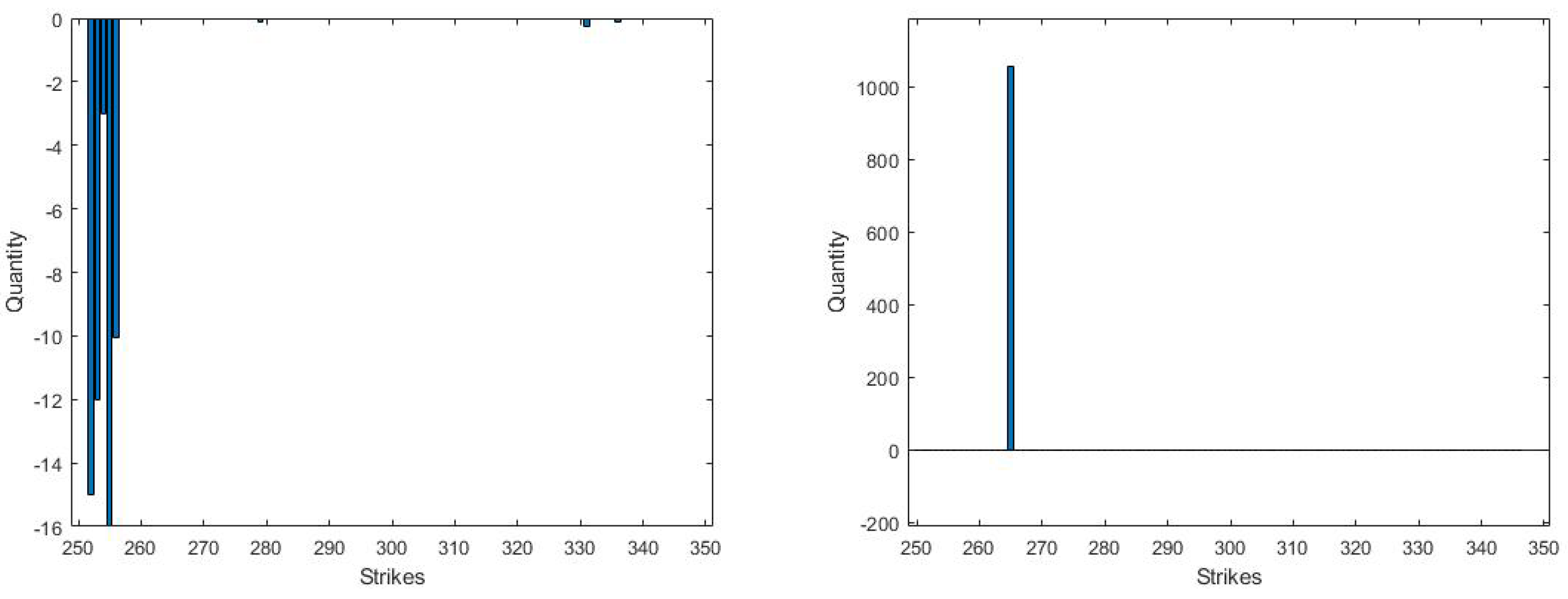
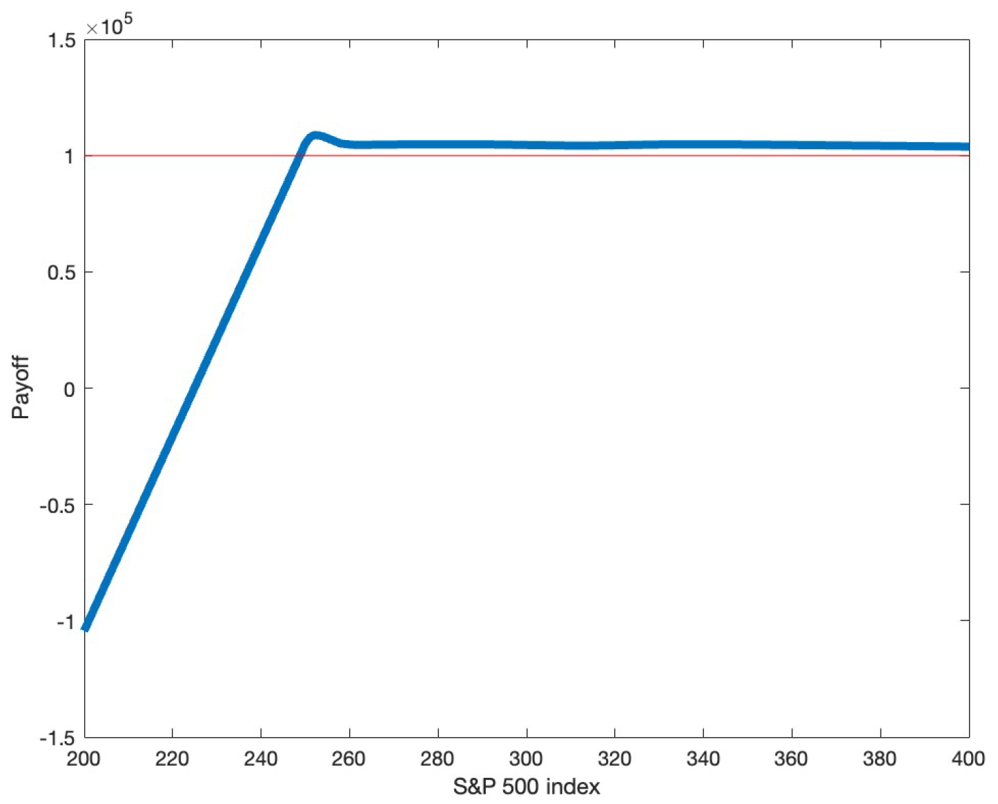
Figure 1 and Figure 2 show the optimized portfolio as well as its payoff as a function of the index value at the expiry date, respectively. The minimum standard derivation (risk) as well as the mean of the payoff obtained with 10,000 out-of-sample simulations of the optimal portfolio are given in

Table 3. The mean and the standard deviation of the optimized portfolio obtained with 10,000 out-of-sample simulations.

Mean	Standard Deviation
105,000.00	1756.98

. The optimization result was obtained using MATLAB version R2022a which took on average 3.7511 seconds on a MacBook Air 13″ with macOS 13.1 Apple M1 8-Core(TM) and 8.00 GB memory.

The left and the right panels of Figure 1 show the optimal quantities taken in put and call options, respectively. It can be seen that the optimization suggests buying a large amount of a call option with strike 265 and selling a relatively smaller amount of the options with multiple strikes from 250–260. This portfolio is guaranteed to have a minimum required return of 5% but has minimal variance given the view of the future value of the index. It is interesting to see, in Figure 2, that the optimal portfolio payoff is above USD 100,000, which is the initial wealth if the index value at the maturity is higher than 250. Note that the current index value is 295.42. This portfolio is considered to be very good as in reality, it is unlikely that the index will fall from 295.42 to below 250 within 30 days. However, if the index at the expiry date falls below 250, the loss increases sharply. This payoff profile is very unlikely to be found for portfolio optimization in spot markets such as those, for example, in [31,33,35].

As shown in Table 3, the mean of the optimized portfolio obtained with 10,000 out-of-sample simulations is USD 105,000. This is not surprising as our required average return is 5%. The standard deviation is USD 1756.98, which is the smallest any portfolio can attain given the required return.

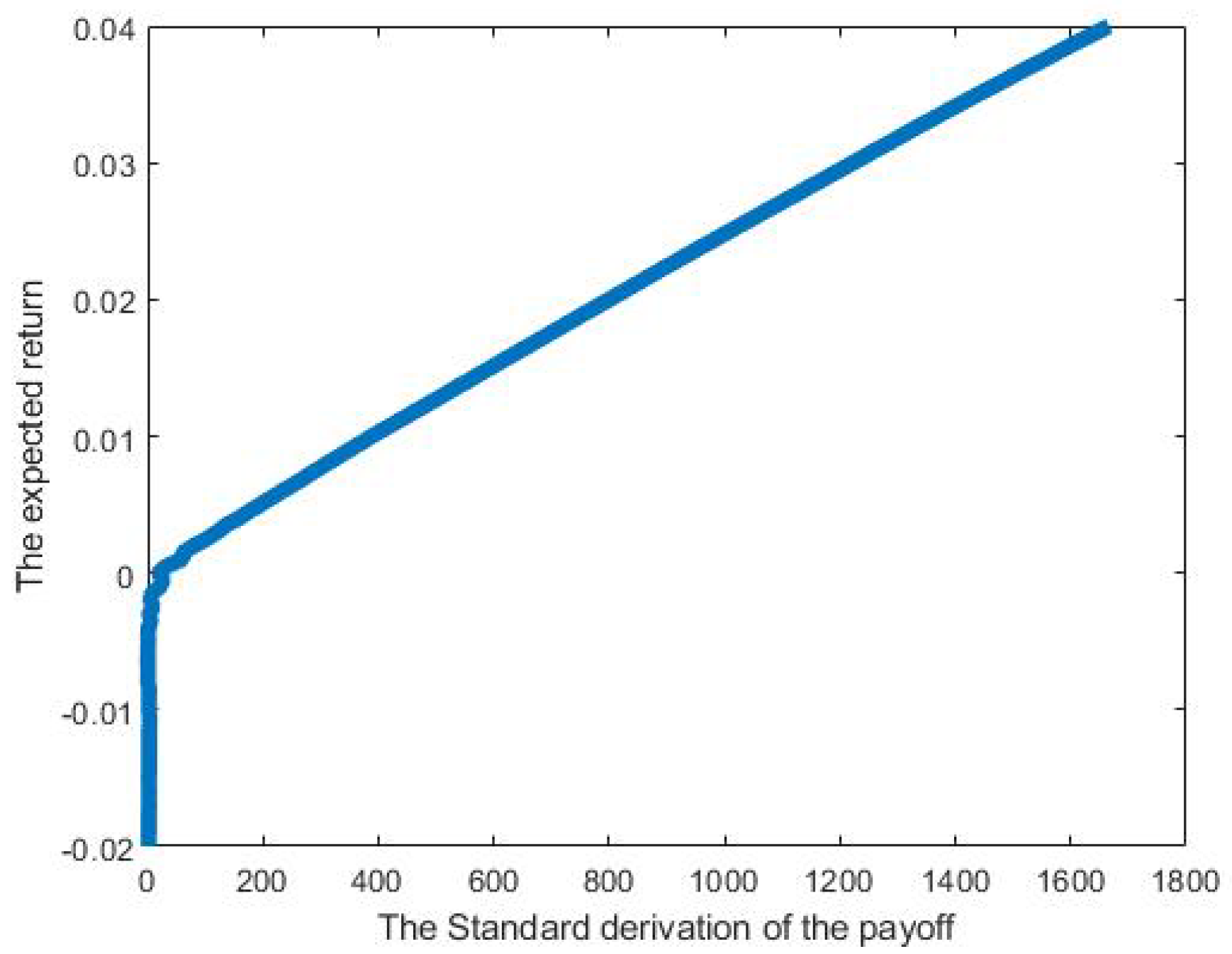
Figure 3 shows the efficient frontier of the standard deviation minimization given bid and ask spreads. The x-axis indicates the standard derivation, whereas the y-axis indicates the level of the expected return. The plot indicates the minimum standard derivation which can be attained given the required average return. We can see that as the required average return increases, the minimum standard deviation (risk) which can be attained also increases. This implies the classic statement in investment, the higher the risk, the higher the return. The shape of the efficient frontier plotted here is standard and similar to those plotted in [36,37,38].

3.1.2. Portfolio Sensitivity

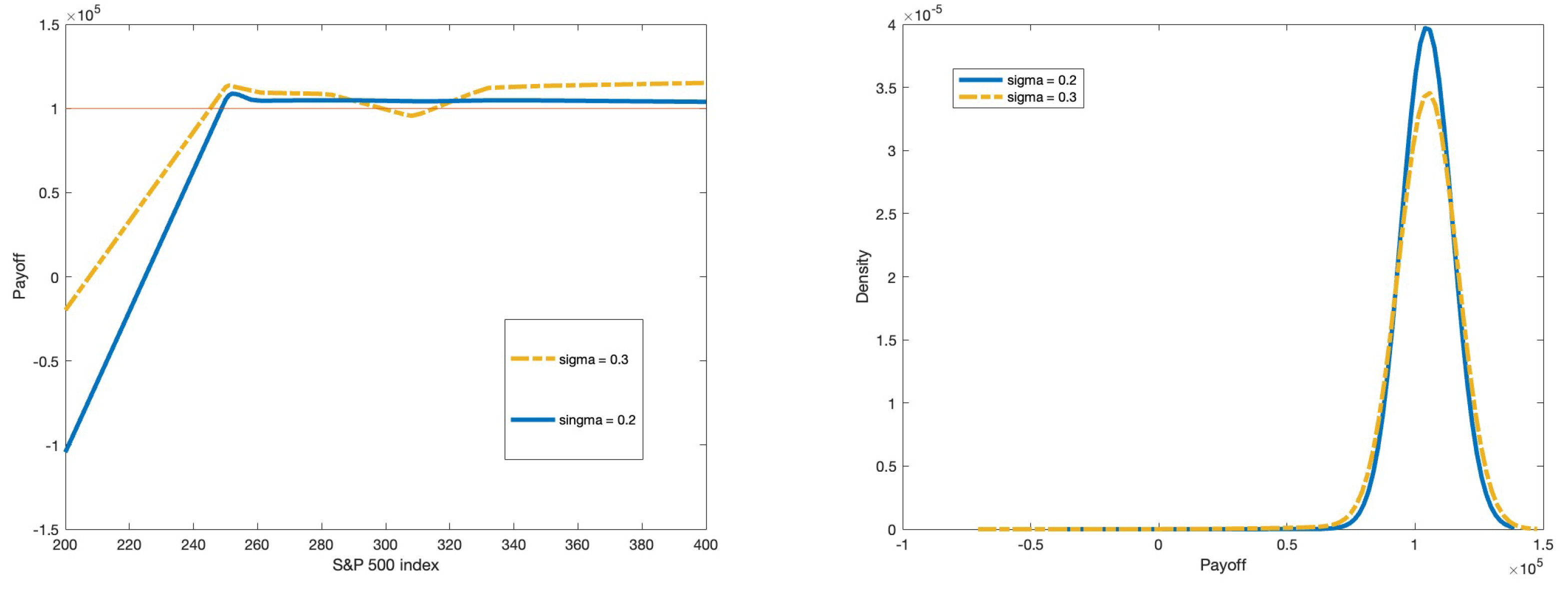
Figure 4 (left) shows the payoffs of the optimized portfolios obtained with different modeling parameters $\sigma$. The blue (solid) line is for $\sigma =0.2$, and the yellow (dashed) line is for $\sigma =0.3$. The required average return is 5%. It can be seen that the optimized portfolio changes according to the probabilistic view. The higher value of the modeling parameter $\sigma$ is, the more volatile the agent believes the value of the index at maturity will be. The payoff for higher volatility (yellow) has a higher payoff at both tails compared with the blue one. It suffers some loss if the index value at maturity is close to the current index value which is more unlikely for higher volatility. It is worth noting that with the higher value of the modeling parameter model $\sigma$, the variance of the payoff of the optimized portfolio becomes bigger (see Figure 4 (right)).

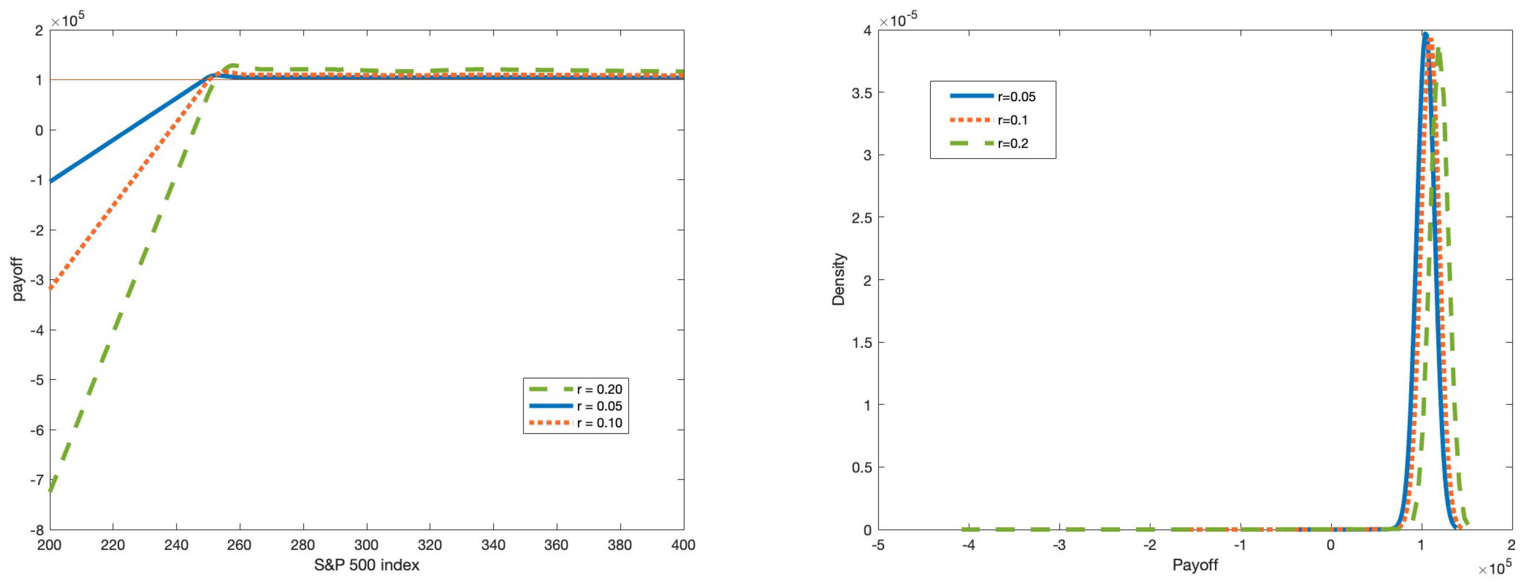
Figure 5 (left) shows the payoffs of the optimized portfolios obtained different required average returns $r=20\%$ (green line, dashed), $r=10\%$ (orange line, dotted), and $r=5\%$ (blue line, solid). We can see that with the higher required average return, the optimized portfolio suffers bigger losses at the left tail. Although the probability that the index value at the expiry date drops significantly below 250 is low, it increases the risk associated with the optimized portfolio. None of the portfolios is better than the other. It after all depends on the required average return the agent needs and the risk he or she can accept. It can be seen on the right panel of Figure 5 that the distribution of the payoff of the optimized portfolio with the higher required return is shifted to the right. This is not surprising as the mean of this payoff must be equal to the required return. However, as you can see, requiring a higher average return results in higher variance (risk) of the optimized portfolio.

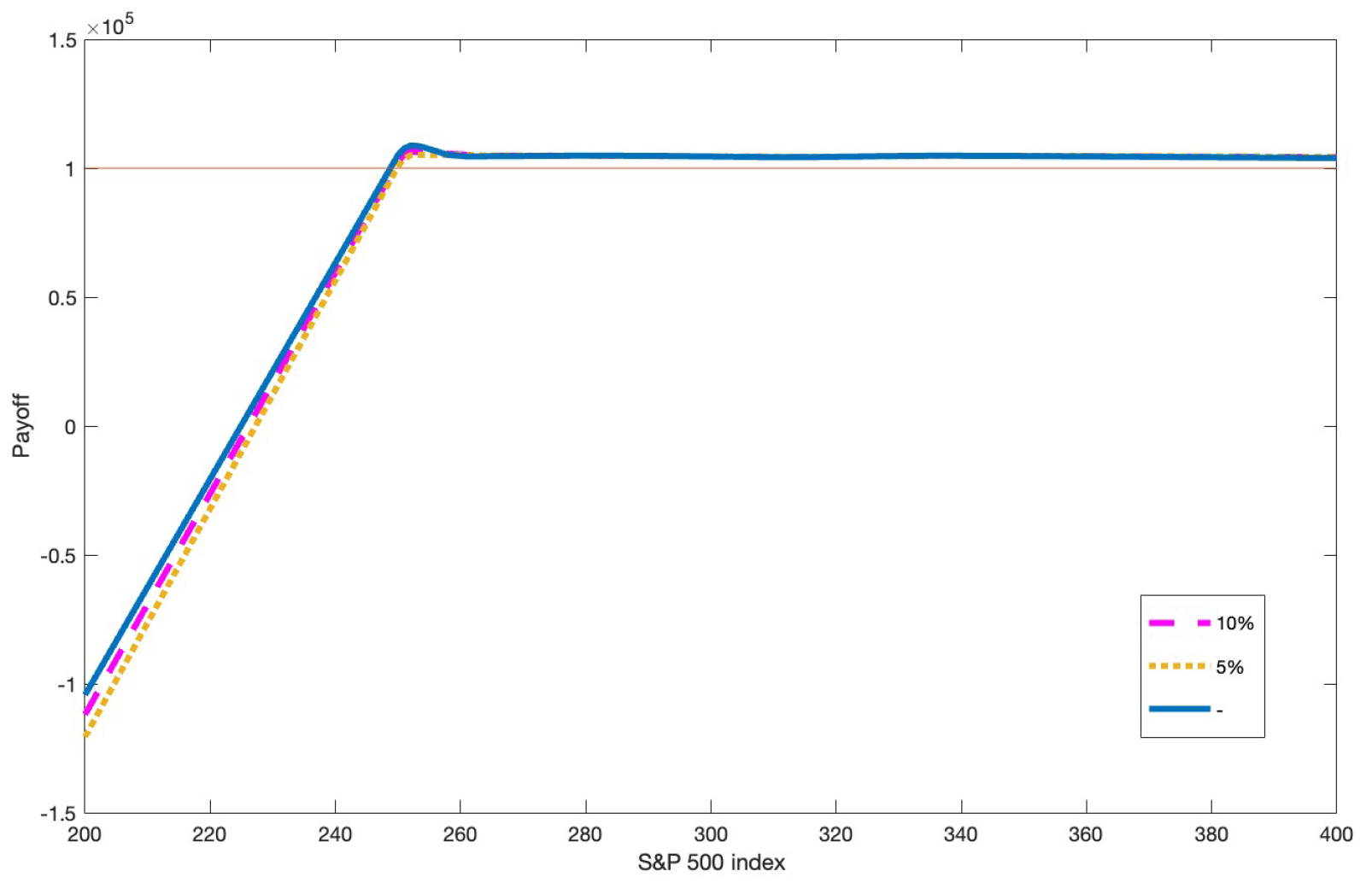
Figure 6 shows the transaction cost of the portfolio payout. We increase the bid–ask spread by adding 5% and 10% transaction costs for all trades. We can see that the graph with transaction cost added has a more negative payoff than non-added transaction cost (where $r=0.05$ and $\sigma =0.2$).

Table 4. The standard deviations of the optimized portfolios obtained with the different values of $\nu$.

$\mathit{\nu }$	Standard Deviation
0.1	5214.13
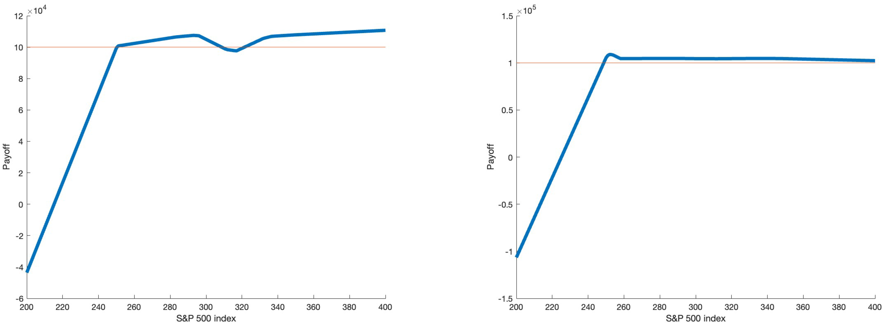
0.00001	1018.50

and Figure 7 show the standard deviation and the payoffs of the optimized portfolios obtained with different values of $\nu$ (the parameter in variance gamma models which has control over kurtosis). The higher the kurtosis, $\nu =0.1$, the greater the value of the risk, and when we lower the kurtosis, $\nu =0.00001$, the value of the risk also decreases. In other words, the fatter the tails are, the harder the investment with low risk is.

3.2. Results: Static Hedging

In this section, we price six difference “exotic” options, namely, an “European call option” with $c\left(S_T\right)=S_T-\kappa$, a “quadratic option” with $c\left(S_T\right)={|S_T-\kappa |}^2$, a “log-option” with $c\left(S_T\right)=1000ln(\kappa /S_T)$, a “digital option” with $c\left(S_T\right)=1000(S_T\ge \kappa )$, a “butterfly spread option” with $c\left(S_T\right)=100((S_T-295)-2(S_T-\kappa )+(S_T-305))$, and “sine option” with $c\left(S_T\right)=1000sin(S_T\times 2\pi /10)$, all with strike $\kappa =300$. Note that the butterfly spread option in the experiment has three strikes at $295,300,305$.

We compute the indifference prices assuming that $\overline{w}$ = 100,000 and $\overline{c}=0$, that is, assuming the agent has an initial position consisting only of 100,000 units of cash. The indifference prices for buying and selling are given in

Table 5. Indifference prices.

Claim	Selling Price	Buying Price
European call option	5.6	5.6
quadratic option	544.5	541.0
log-option	38.8	38.5
digital option	513.4	462.5
butterfly spread option	68.7	54.8
sine option	351.9	0.1

.

Figure 8, Figure 9, Figure 10, Figure 11, Figure 12 and Figure 13 illustrates the hedging portfolios for the sale of all exotic options mentioned above and compare the payouts of the hedging portfolios as functions of the index value at the maturity with the payouts of the exotic options. One can see that the hedging portfolio replicates the payout of the sold option reasonably well under the incompleteness of the market. We can see that the hedging portfolios try to replicate the payoffs of the sold options, especially at the values of the index with a higher probability of occurring. This is because we are minimizing the variance of the difference between the hedging portfolio payoff and the sold option payoff. The difference between the two where the probability of occurring is low does not significantly affect the overall variance. Note that if the payout of the hedging portfolio is above that of the sold option, the seller will end up with some profit. Because the seller enters this hedging portfolio after receiving the selling price from the buyer. If the payout of the hedging portfolio is higher than that of the sold option, the seller will have some money left after paying the buyer. In practice, the seller may charge an additional amount which makes the hedging portfolio payoff higher. This will reduce the risk where the hedging portfolio payout is less than that of the sold option.

It is noticeable that there are residuals in the hedgings. This is not the case in the Black and Scholes framework in which standard put and call options can be hedged with just it’s underlying and a bank account, see [4]. In such a framework, the completeness of the market is assumed. Comparing the results with the Breeden–Litzenberger formula carried out in [25] which provides an approximation formula for pricing and hedging exotic options incomplete markets which normally includes holding many standard put and call options for hedging, our hedging portfolio consists of just a few options. This is very important in practice as it is much more inconvenient and more expensive to take a position in many options. In addition, our scheme looks for the best combination of assets subject to the agent’s view, initial position, and required return. Compared with the work by Armstrong et al. [27,28] where the risk is measured by the exponential loss function, the hedging portfolio under mean-variance criteria focuses more on reducing the deviation of the hedging portfolio payout from that of the exotic option than to make a profit. Unlike the exponential loss utility, which is more sensitive to the loss, for mean-variance criteria, the discrepancy on both profit and loss sides is equally minimized. Whether or not this hedging scheme is better is subjective. Some users may focus more on perfect hedging where the hedging payoff is as close as possible to that of the exotic option. However, some may be willing to sacrifice the low discrepancy for the opportunity to make more profit.

4. Conclusions

In this paper, we propose a scheme to compute indifference prices and the hedging portfolios for financial derivatives in incomplete markets where the quotes come with finite liquidity and bid–ask spreads. The scheme is built upon the modified mean-variance portfolio optimization model as computing the indifference prices is the same as iteratively solving the optimal investment problems. We illustrate the application of the scheme in the S&P 500 mini options market where the tradable assets are cash, and 199 mini put and call options written on the S&P 500 index. The index return is modeled by the variance gamma process which gives the user control over the skewness and kurtosis.

We first solve the portfolio optimization problem and demonstrate the effects of various parameters such as modeling parameters and the required average return on the optimal portfolio and its payoff. After that, we compute the indifference prices for six exotic options which are a “European call option”, a “quadratic option”, a “log-option”, a “digital option”, a “butterfly spread option”, and a “sine option”. We show that the hedging portfolios obtained under this scheme provide decent approximations of the payoffs of exotic options. This method can be an alternative to the classical derivatives pricing under the Black and Scholes framework where all assets are assumed to be perfectly liquid, ignoring bid and ask spreads as well as the limited available quantities for buying and selling, which is not true in general. The six options priced here are just examples. In addition, as opposed to the risk-neutral pricing and hedging scheme where it is very unlikely to have solutions for complex derivatives, the method illustrated herein can also be applied to price any exotic derivatives with explicit payoff functions. It can also be easily applied in any other financial market apart from the S&P 500 market by just changing the input data and the appropriate stochastic model used in the simulation.

The scheme herein can be improved in many aspects. First, the optimization is too slow. By the time we finish the computation, the bid and ask prices and available sizes of some assets might already have changed which renders the hedging portfolio not optimal or not attainable. This can be improved by using an integral quadrature instead of Monte Carlo simulations to estimate the objective function. As the density of the process is known, the variance of the terminal loss can be expressed in terms of an integration that can be approximated more efficiently with an integral quadrature reducing the simulation time as well as the optimization problem size resulting in the reduction in overall computational time. Another improvement is to include more than one random factor in the problem. As seen in the Data section, we only have options written on a single index. The problem can become more interesting if the data includes options in multiple markets such as options written on S&P 500 index and options written on VIX. The challenge is to come up with a sensible stochastic process to jointly model the two random factors.

References

1. Liu, C.; Chang, C.; Chang, Z. Maximum Varma entropy distribution with conditional value at risk constraints. Entropy 2020, 22, 663. [Google Scholar] [CrossRef] [PubMed]
2. Maheshwari, A.; Pirvu, T.A. Portfolio optimization under correlation constraint. Risks 2020, 8, 15. [Google Scholar] [CrossRef]
3. Wang, D.; Chen, Y.; Wang, H.; Huang, M. Formulation of the non-parametric value at risk portfolio selection problem considering symmetry. Symmetry 2020, 12, 1639. [Google Scholar] [CrossRef]
4. Black, F.; Scholes, M. The pricing of options and corporate liabilities. J. Political Econ. 1973, 81, 637–654. [Google Scholar] [CrossRef]
5. Pennanen, T. Introduction to convex optimization in financial markets. Math. Program. 2012, 134, 157–186. [Google Scholar] [CrossRef]
6. Pennanen, T. Optimal investment and contingent claim valuation in illiquid markets. Financ. Stochastics 2014, 18, 733–754. [Google Scholar] [CrossRef]
7. Nonsoong, P.; Mekchay, K.; Rujivan, S. An analytical option pricing formula for mean-reverting asset with time-dependent parameter. ANZIAM J. 2021, 63, 178–202. [Google Scholar]
8. Chumpong, K.; Tanadkithirun, R.; Tantiwattanapaibul, C. Simple closed-form formulas for conditional moments of inhomogeneous nonlinear drift constant elasticity of variance process. Symmetry 2022, 14, 1345. [Google Scholar] [CrossRef]
9. Chumpong, K.; Sumritnorrapong, P. Closed-form formula for the conditional moments of log prices under the inhomogeneous Heston model. Computation 2022, 10, 46. [Google Scholar] [CrossRef]
10. Rujivan, S.; Rakwongwan, U. Analytically pricing volatility swaps and volatility options with discrete sampling: Nonlinear payoff volatility derivatives. Commun. Nonlinear Sci. Numer. Simul. 2021, 100, 105849. [Google Scholar] [CrossRef]
11. Sutthimat, P.; Mekchay, K. Closed-form formulas for conditional moments of inhomogeneous Pearson diffusion processes. Commun. Nonlinear Sci. Numer. Simul. 2022, 106, 106095. [Google Scholar] [CrossRef]
12. Chumpong, K.; Mekchay, K.; Thamrongrat, N. Analytical formulas for pricing discretely-sampled skewness and kurtosis swaps based on Schwartz’s one-factor model. Songklanakarin J. Sci. Technol. 2021, 43, 1–6. [Google Scholar]
13. Chumpong, K.; Mekchay, K.; Rujivan, S. A simple closed-form formula for the conditional moments of the Ornstein–Uhlenbeck process. Songklanakarin J. Sci. Technol. 2020, 42, 836–845. [Google Scholar]
14. Duangpan, A.; Boonklurb, R.; Chumpong, K.; Sutthimat, P. Analytical formulas for conditional mixed moments of generalized stochastic correlation process. Symmetry 2022, 14, 897. [Google Scholar] [CrossRef]
15. Chumpong, K.; Mekchay, K.; Rujivan, S.; Thamrongrat, N. Simple analytical formulas for pricing and hedging moment swaps. Thai J. Math. 2022, 20, 693–713. [Google Scholar]
16. Sepp, A. Pricing options on realized variance in the Heston model with jumps in returns and volatility. J. Comput. Financ. 2008, 11, 33–70. [Google Scholar] [CrossRef]
17. Boonklurb, R.; Duangpan, A.; Rakwongwan, U.; Sutthimat, P. A novel analytical formula for the discounted moments of the ECIR process and interest rate swaps pricing. Fractal Fract. 2022, 6, 58. [Google Scholar] [CrossRef]
18. Nualsri, F.; Mekchay, K. Analytically pricing formula for contingent claim with polynomial payoff under ECIR process. Symmetry 2022, 14, 933. [Google Scholar] [CrossRef]
19. Sutthimat, P.; Rujivan, S.; Mekchay, K.; Rakwongwan, U. Analytical formula for conditional expectations of path-dependent product of polynomial and exponential functions of extended Cox–Ingersoll–Ross process. Res. Math. Sci. 2022, 9, 1–17. [Google Scholar] [CrossRef]
20. Sutthimat, P.; Mekchay, K.; Rujivan, S. Closed-form formula for conditional moments of generalized nonlinear drift CEV process. Appl. Math. Comput. 2022, 428, 127213. [Google Scholar] [CrossRef]
21. Sutthimat, P.; Mekchay, K.; Rujivan, S. Explicit formula for conditional expectations of product of polynomial and exponential function of affine transform of extended Cox–Ingersoll–Ross process. J. Physics: Conf. Ser. 2018, 1132, 012083. [Google Scholar] [CrossRef]
22. Monoyios, M. Utility indifference pricing with market incompleteness. In Nonlinear Models in Mathematical Finance: New Research Trends in Option Pricing; Ehrhardt, M., Ed.; Nova Science Publishers: Hauppauge, NY, USA, 2008; pp. 67–100. [Google Scholar]
23. Musiela, M.; Zariphopoulou, T. An example of indifference prices under exponential preferences. Financ. Stochastics 2004, 8, 229–239. [Google Scholar] [CrossRef]
24. Pennanen, T.; Perkkiö, A.P. Convex duality in optimal investment and contingent claim valuation in illiquid markets. Financ. Stochastics 2018, 22, 733–771. [Google Scholar] [CrossRef]
25. Breeden, D.T.; Litzenberger, R.H. Prices of state-contingent claims implicit in option prices. J. Bus. 1978, 51, 621–651. [Google Scholar] [CrossRef] [Green Version]
26. Madan, D.; Seneta, E. The variance gamma (VG) model for share market. J. Bus. 1990, 63, 511–524. [Google Scholar] [CrossRef]
27. Armstrong, J.; Pennanen, T.; Rakwongwan, U. Pricing index options by static hedging under finite liquidity. Int. J. Theor. Appl. Financ. 2018, 21, 1850044. [Google Scholar] [CrossRef]
28. Pennanen, T.; Bonatto, L.S. A stochastic oil price model for optimal hedging and risk management. Int. J. Theor. Appl. Financ. 2022, 25, 2250009. [Google Scholar] [CrossRef]
29. v Puelz, A. Value-at-risk based portfolio optimization. In Stochastic Optimization: Algorithms and Applications; Springer: Berlin/Heidelberg, Germany, 2001; pp. 279–302. [Google Scholar]
30. Gaivoronski, A.A.; Pflug, G. Value-at-risk in portfolio optimization: Properties and computational approach. J. Risk 2005, 7, 1–31. [Google Scholar] [CrossRef]
31. Rockafellar, R.T.; Uryasev, S. Optimization of conditional value-at-risk. J. Risk 2000, 2, 21–42. [Google Scholar] [CrossRef]
32. Maasar, M.A.; Roman, D.; Date, P. Portfolio optimisation using risky assets with options as derivative insurance. In 5th Student Conference on Operational Research (SCOR 2016); Schloss Dagstuhl-Leibniz-Zentrum fuer Informatik: Wadern, Germany, 2016. [Google Scholar]
33. Markowitz, H. Portfolio Selection. J. Financ. 1952, 7, 77–91. [Google Scholar]
34. Madan, D.B.; Carr, P.P.; Chang, E.C. The variance gamma process and option pricing. Rev. Financ. 1998, 2, 79–105. [Google Scholar] [CrossRef]
35. Marakbi, Z. Mean-Variance Portfolio Optimization: Challenging the Role of Traditional Covariance Estimation. 2016. Available online: http://urn.kb.se/resolve?urn=urn:nbn:se:kth:diva-199185 (accessed on 23 March 2017).
36. Michaud, R.O. The Markowitz optimization enigma: Is ‘optimized’optimal? Financ. Anal. J. 1989, 45, 31–42. [Google Scholar] [CrossRef]
37. Das, S.; Markowitz, H.; Scheid, J.; Statman, M. Portfolios for investors who want to reach theirgoals while staying on the mean–variance efficient frontier. J. Wealth Manag. 2011, 14, 25–31. [Google Scholar] [CrossRef] [Green Version]
38. Kosapong, B.; Boonserm, P.; Rakwongwan, U. Options portfolio optimization of exotic options written on Mini S&P500 Index in an illiquid market with Conditional Value-at-Risk (CVaR). Thai J. Math. 2022, 169–183. Available online: http://thaijmath.in.cmu.ac.th/index.php/thaijmath/article/view/6118 (accessed on 31 March 2022).
Figure 1. Optimized portfolio in the put options (left) and the call options (right).
Computation 11 00030 g001
Figure 2. The payoffs of the optimal portfolios as functions of the S&P 500 index.
Computation 11 00030 g002
Figure 3. The coefficient frontier of the variance minimization.
Computation 11 00030 g003
Figure 4. The payoffs of the optimized portfolios as functions of the index value at the expiry date obtained with σ = 0.2 and σ = 0.3 (left), and the kernel density of the payoff of at the optimized portfolios obtained with 10,000 out-of-sample simulations (right).
Computation 11 00030 g004
Figure 5. The minimum standard deviation of the portfolio payout distribution with r = 0.2 , 0.1 , 0.05 (left), the kernel density estimation of the portfolio payout with r = 0.2 , 0.1 , 0.05 (right).
Computation 11 00030 g005
Figure 6. The transaction cost of the portfolio payout.
Computation 11 00030 g006
Figure 7. The payoffs of the optimized portfolios obtained with ν = 0.1 (left) and ν = 0.00001 (right).
Computation 11 00030 g007
Figure 8. The payoff of the hedging portfolio together with the payoff of the claim being priced of a call option (left), the hedging portfolios for the put option (center) and call option (right).
Computation 11 00030 g008
Figure 9. The payoff of the hedging portfolio together with the payoff of the claim being priced of a quadratic option (left), the hedging portfolios for the put option (center) and call option (right).
Computation 11 00030 g009
Figure 10. The payoff of the hedging portfolio together with the payoff of the claim being priced of a log-option (left), the hedging portfolios for the put option (center) and call option (right).
Computation 11 00030 g010
Figure 11. The payoff of the hedging portfolio together with the payoff of the claim being priced of a price digital (left), the hedging portfolios for the put option (center) and call option (right).
Computation 11 00030 g011
Figure 12. The payoff of the hedging portfolio with the payoff of the claim being priced of a butterfly spread option (left), the hedging portfolios for the put option (center) and call option (right).
Computation 11 00030 g012
Figure 13. The payoff of the hedging portfolio together with the payoff of the claim being priced of a sine option (left), the hedging portfolios for the put option (center) and call option (right).
Computation 11 00030 g013