Measuring the Recovery Performance of a Portfolio of NPLs

Abstract

The objective of the present paper is to propose a new method to measure the recovery performance of a portfolio of non-performing loans (NPLs) in terms of recovery rate and time to liquidate. The fundamental idea is to draw a curve representing the recovery rates over time, here assumed discretized, for example, in years. In this way, the user can get simultaneously information about recovery rate and time to liquidate of the portfolio. In particular, it is discussed how to estimate such a curve in the presence of right-censored data, e.g., when the NPLs composing the portfolio have been observed in different time periods, with a method based on an algorithm that is usually used in the construction of survival curves. The curves obtained are smoothed with nonparametric statistical learning techniques. The effectiveness of the proposal is shown by applying the method to simulated and real financial data. The latter are about some portfolios of Italian unsecured NPLs taken over by a specialized operator.

1. Introduction

Non-performing loans (hereafter, NPLs) are, in the main category of loans whose collection by banks is uncertain, exposures in a state of insolvency.

As Resti and Sironi [1] underline, an effective recovery depends on a series of factors, peculiar to the credit (presence of guarantees, etc.), peculiar to the counterparty (sector, country, etc.), peculiar to the creditor (such as the efficiency in recovering money), as well as macroeconomic factors such as the state of the economy.

There is an NPL market that offers banks the opportunity to get rid of non-performing loans by selling them to specialized operators who deal with recovery.

The main method for determining the value of non-performing loans is that of discounted financial flows, according to which the value of the loans is equal to the sum of the expected income flows, discounted at a rate consistent with the expected unlevered return of the investor and net of the related recovery costs.

In the case of a performing loan, the borrower is expected to pay principal and interest at the agreed deadlines with a high level of probability (one minus the probability of default, generally low). In this case, the uncertainty in the valuation is limited to the determination of the discount rate, which takes into account the general market circumstances of the rates and the specific risk of the debtor.

In the case of non-performing loans, the uncertainty concerns not only the discount rate but also the amount that will be returned and the time of return. In fact, the probability of default is now equal to one, in the case in which the transition to non-performing loans has already occurred, or is in any case very high, if the credit is in the other categories of impaired loans (unlikely to pay).

The valuation methodologies currently used on the market are therefore based primarily on forecast models of the amount of net repayments expected from receivables and related collection times. The operation is not trivial and is carried out with different models. The choice of how to model the expected net flows essentially depends on the type of credit and on the information available to the evaluator. It is first necessary to consider whether a real guarantee (typically a mortgage or pledge) on an existing asset with a market value covers the credit. In this case, the flow forecast model is based on the lesser of the value of the asset covered by the guarantee, the amount of the guarantee, and the value of the credit, and on the timing for its judicial sale. The valuation methods to be applied are those based mainly on the compulsory recovery of the credit, while also providing for the possibility of recovering the credit through an out-of-court agreement in some cases.

Forecast models are generally based on: the information available to the creditor, public information, and information acquired and processed as part of the analysis.

The availability of one type of information over another radically changes the articulation and degree of detail that the evaluator can give to the flow forecasting models and consequently to the evaluation methods.

The forecast models with the aforementioned limits use all the relevant information available to determine the estimated flows and related timing. They can be traced back to three types, which can be partially combined with each other: models based on judicial recovery, models based on the debtor’s restitution capacity, and statistical forecasting models.

The estimation methodology for recovery rate, which we are interested in for NPLs, was addressed in the more general context of Basel II. The Basel Committee proposed an internal ratings-based (IRB) approach to determining capital requirements for credit risk [2,3]. This IRB approach allows banks to use their own risk models to calculate regulatory capital. According to the IRB approach, banks are required to estimate the following risk components: probability of default (PD), loss given default (LGD), exposure to default (EAD), and maturity (M). Given that LGD has a large impact on the calculation of the capital requirement, financial institutions have placed greater emphasis on modeling this quantity. In any case, LGD modeling for banks is important because it is useful for internal risk monitoring and pricing credit risk contracts, although internal modeling of LGD and EAD for regulatory purposes will soon be limited [4,5].

Given that the borrower has already defaulted, LGD is defined as the proportion of money financial institutions fail to gather during the collection period, and conversely, recovery rate (RR) is defined as the proportion of money financial institutions successfully collect. That means LGD = 1 − RR. Despite the importance of LGD, little work has been done on it in comparison to PD, as summarized below.

The recovery rate (or LGD) can be estimated using both parametric and non-parametric statistical learning methods. Mainly, the recovery rate is estimated using parametric methods and considering a one-year time horizon.

Methods used in literature, among others, are: classical linear regression, regularized regression such as Lasso, Ridge, Elastic-net, etc. [6], support vector regression [7], beta regression, inflated beta regression, two-stage model combining beta mixture model with a logistic regression model [8], and other machine learning methods [9,10,11,12].

Recently, in order to compare different methods to model the recovery rate, in [13] authors give an overview of the existing literature with focus on regression models, decision trees, neural networks and mixture models and reach the conclusion that the latter approach is the one giving the better results.

Reference papers for a comprehensive overview of regression models, neural networks, regression trees, and similar approaches are the comparative studies of [14], who conclude that non-linear techniques, and in particular support vector machines and neural networks, perform significantly better than more traditional linear techniques, and [15], who state that non-parametric methods (regression tree and neural network) perform better than parametric methods.

Among parametric models, linear regression is the most common and simplest technique used to predict the mean, whereas to model the overall LGD distribution, or at least certain quantiles of it, linear quantile regression [16,17] and mixture distributions [8,18,19,20,21,22] are proposed.

Due to interest payments, high collateral recoveries, or administrative and legal costs, the LGD value can exceed one or be below zero. A way to solve these cases can be multistage modeling, as for instance in [23]. Other evidence of multistage models is in [7,24,25,26].

In the case of NPLs, in our opinion, in investigating the recovery process of defaulted exposures the focus must be not only on the recovered amounts but also on the duration of the recovery process, the so-called time to liquidate (TTL), and we believe that this type of approach needs to be explored further.

Devjak [27] refers to both size and time of future repayments in a simple model only considering NPLs for which the recovery process was finished. Cheng and Cirillo [10] propose a model that can learn, using a Bayesian update in a machine learning context, how to predict the possible recovery curve of a counterpart. They introduce a special type of combinatory stochastic process based on a complex system of assumptions, referring to a discretization of recovery rates in m levels. Betz, Kellner, and Rosch [28] develop a joint modeling framework for default resolution time (duration of loans) and LGD, also considering the censoring effects of unresolved loan contracts. They develop a hierarchical Bayesian model for joint estimation of default resolution time and LGD, including survival modeling techniques applicable to duration processes. Previous examples of the usage of survival techniques to study the impact of the duration of loans on LGD are in [29,30,31].

Our purpose is to study a particular nonparametric method to measure the performance of an NPL portfolio in terms of recovery rate (RR) and time to liquidate (TTL) jointly, without assuming any particular model and/or discretization of the RR. The idea is to represent the recovery process as a curve showing how the RR is distributed over time without assuming a particular parametric model. We will also consider a method to estimate such a curve when some data are censored, i.e., when the repayment history for some NPLs is known only until a particular data. The algorithm we propose corresponds to applying the actuarial mortality tables method [32] by considering each currency unit as an individual, and it can be considered a different motivation from the approach exploited in [30]. The actuarial mortality tables method has been applied in [33] in the context of corporate bonds and in [29] for an NPL portfolio owned by a Portuguese bank. In this paper, we go beyond these works in several directions. Firstly, by smoothing the curve by using non-parametric statistical learning techniques. Secondly, by testing the performance of the proposal through a simulation study that is compared with other methods. Finally, by applying our method to real financial data consisting of two large NPL portfolios dismissed by banks and taken over by a specialized operator. To our best knowledge, there are no published studies analyzing the recovery rate timing of this kind of NPLs. This analysis will reveal important differences with the results obtained in [29] for an NPL portfolio owned by a bank.

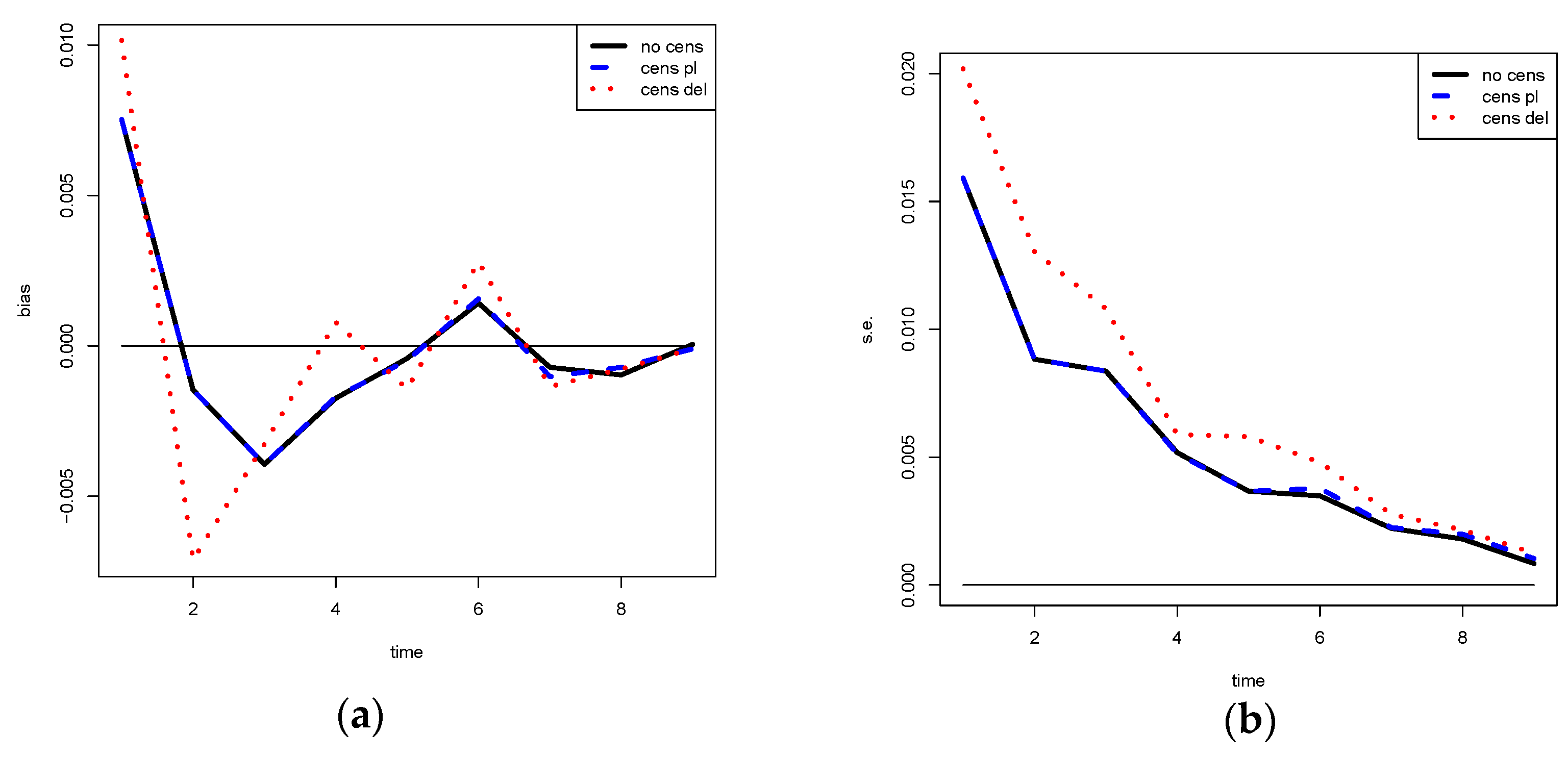
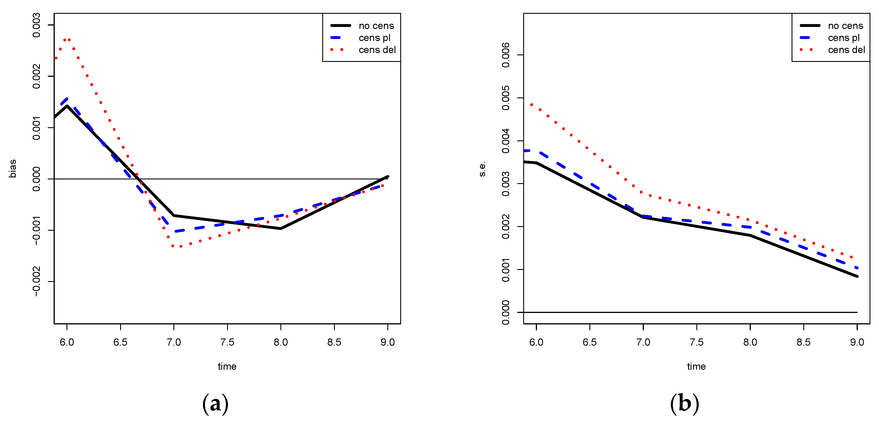
The plan of the paper is the following: In Section 2.1, we show how the recovery curve is defined. The method of estimation in the case of censored data is discussed in Section 2.2 and improved in Section 2.3 by smoothing the curves by using regression splines. In Section 3.1, the effectiveness of the proposal is shown through a simulation study. In Section 3.2, we apply our method to real data, while some conclusions and final remarks are discussed in Section 4.

This is the full paper version of [34] and a completion of the working paper [35].

2. Materials and Methods

2.1. Recovery Rate and Time to Liquidate of a Portfolio

The definition and computation of RR and TTL of an NPL portfolio are not trivial because the two quantities are strictly related. To make clear what we mean by “recovery rate” and “time to liquidate” and how they are related in the case of a portfolio, we have to answer several questions about the RR. For example: when do we measure the RR? When the last NPL in the portfolio has been liquidated or after a given period? Moreover, in the latter case, how do we choose the length of the period? Similarly, for the TTL: when do we measure the TTL? When the last NPL has been liquidated or when a significant part of the portfolio has been recovered? Finally, in the latter case, how much is the significant part?

The above questions make clear that the measurement of the RR cannot disregard the measurement of the TTL and vice versa. How do we deal with this problem?

Since it is crucial to decide when to measure the RR and TTL—that is, when each NPL in the portfolio has been entirely liquidated or after a given period to be defined—the measurement of the RR cannot disregard the measurement of the TTL and vice versa.

First, we note that measuring the TTL when the last NPL has been liquidated could lead to measures that are highly affected and biased by anomalous NPLs with long TTLs and small EAD. It follows that the TTL should be measured when the RR becomes significant. It remains to understand what is “significant”. Second, in many cases, the user needs more complete information rather than only two numbers: RR and TTL. It would be better to know how the RR increases over time. This would also help in choosing at what RR point to measure the TTL. For the aforementioned reasons, we decided to measure the behavior of the RR over time through what we called the “recovery curve”. Such a curve is built in the following way.

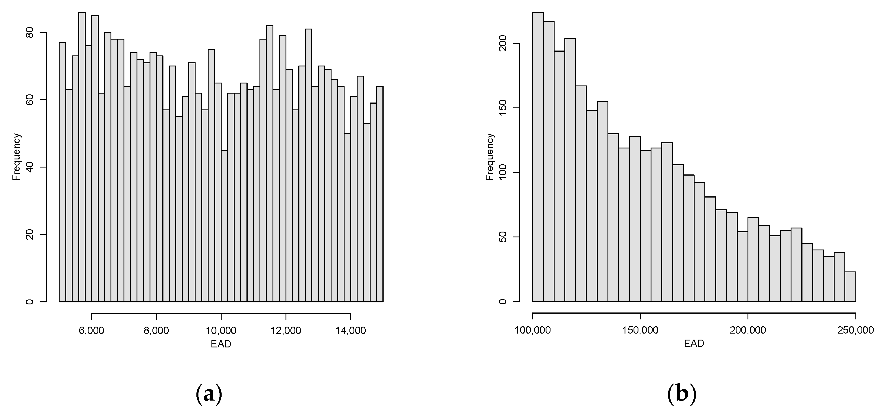
Let us consider a portfolio of $K$ NPLs. For each of the $K$ NPLs, the debt exposure at default is $EA{D}_k$ (exposure at default of the $k-th$ NPL) and the total exposure for the portfolio is $EAD={{\displaystyle \sum }}_{k=1}^{K}EA{D}_k$. Assume $T$ discrete-time intervals of equal length (of the delay of payment) from the default, in time $t=0$, to time $t=T$, i.e., the valuation date. Let $p_{k,t}$ be the recovery of the $k-th$ NPL, in the $t-th$ interval (of delay), i.e., $\left(t-1,t\right]$, with $k \in \left\{1, 2, \dots , K\right\}$ and $t \in \left\{1, 2, \dots , T\right\}$. The portfolio recovery in time interval $t$ equals $p_t={{\displaystyle \sum }}_{k=1}^K{p}_{k,t}$, that is the total recovery, for all the $K$ debt positions, in the $t-th$ time interval of delay. Consequently, after $t$ time intervals of delay, i.e., by the end of the interval $\left(0,t\right]$, we define

$$P_t={\displaystyle \sum }_{i=1}^t{p}_i$$

(1)

as the total portfolio “recovery value until time t”, i.e., the total recovery, for all the $K$ debt positions, in the first $t$ periods from the default date.

We could also define the total recovery $P_t^{*}={{\displaystyle \sum }}_{i=1}^t{\mathrm{V}(p}_i)$, being $\mathrm{V}\left(p_t\right)$ the value of $p_t$ evaluated at an appropriate interest rate, since in measuring the recovery rate the net cash flows must be finally discounted with a discount rate appropriately reflecting the risk [36]. Anyway, in this initial study, we (like many others, i.e., [8,27]) do not consider any discounting because we consider recovery time and recovery rate jointly, because the recovery curve, even if lower, would have the same trend, and—above all—because we can consider the discounted values in a future version of the work.

We define

$$R_t=\frac{P_t}{EAD}$$

(2)

as the portfolio “recovery rate until time $t$”, while

$$r_t=\frac{p_t}{EAD}$$

(3)

equals the portfolio recovery rate in the $t-th$ time interval of delay $\left(t-1,t\right]$.

Since $R_t={{\displaystyle \sum }}_{i=1}^t{r}_i$ we can refer in an equivalent way to $R_t$ or to $r_t$, being $r_t=R_t-R_{t-1}$ (for $t=2, \dots , T$) and $r_1=R_1$.

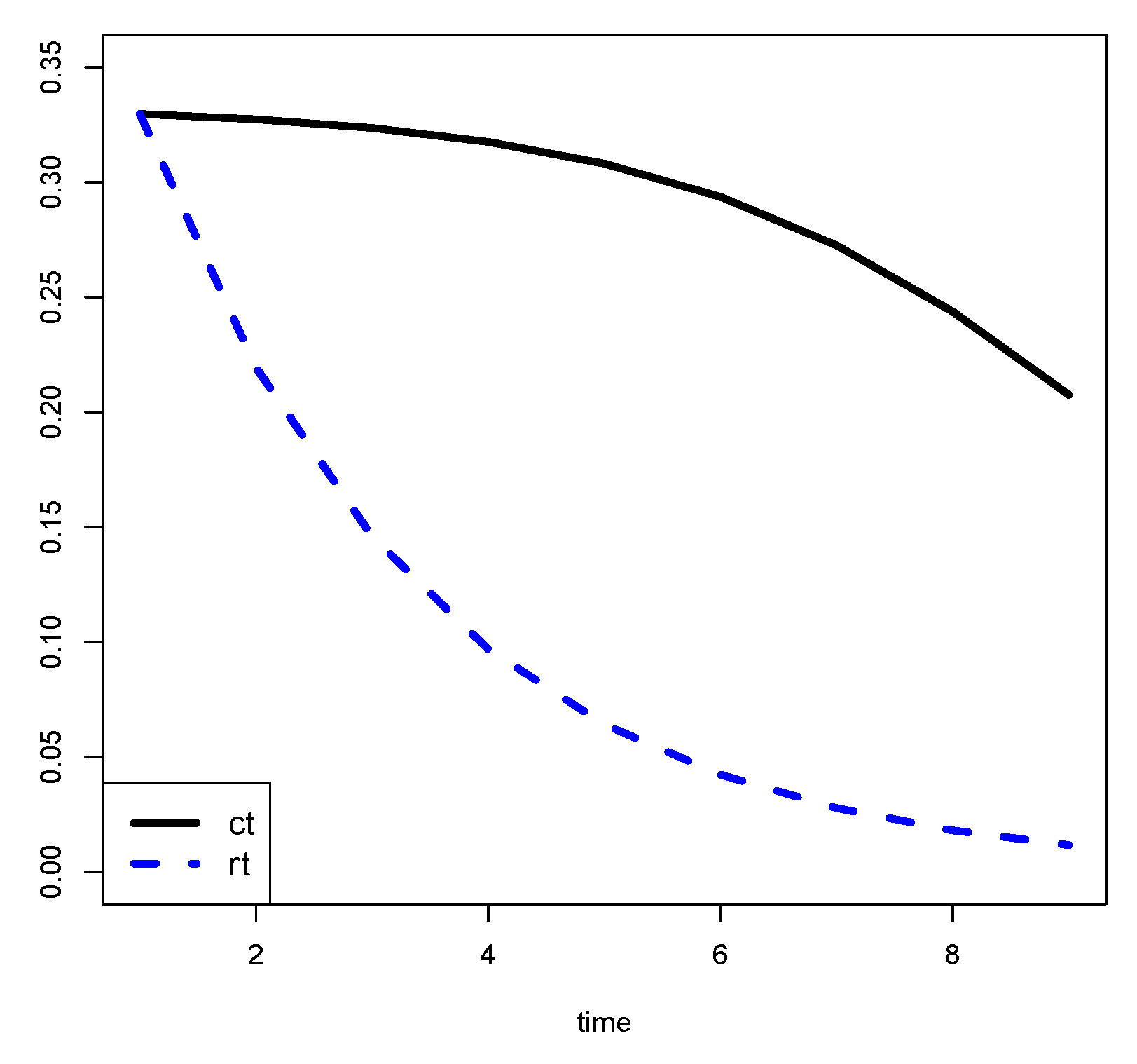
Let us consider the following example.

Consider a portfolio with $K=4$ debt positions. We are interested in measuring its performances in $3$ years after default, i.e., $T=3$ periods of delay.

The data are in the following

Table 1. Portfolio with $K=4$ debt positions and $3$ periods of delay.

$\mathit{k}$	$\mathit{E}\mathit{A}{\mathit{D}}_{\mathit{k}}$	${\mathit{p}}_{\mathit{k},1}$	${\mathit{p}}_{\mathit{k},2}$	${\mathit{p}}_{\mathit{k},3}$
1	100	10	0	0
2	200	20	15	0
3	300	20	25	10
4	400	30	35	10

.

The portfolio performance can be measured in terms of recovery rates until year t (R_t) as shown in

Table 2. Portfolio ($EAD=1000$ ) performance in 3 years ($T=3$ ).

$\mathit{t}$	1	2	3
$p_t$	80	75	20
$P_t$	80	155	175
$r_t$	8.00%	7.50%	2.00%
$R_t$	8.00%	15.50%	17.50%

.

We see that, for example, in the first 2 years, the portfolio recovers 15.5% of the total initial exposure: 8% in the first year and 7.5% in the second.

Sometimes the available data are incomplete, in particular right censored, because the $p_{k,t}$ is not available from a particular date on for some $k$. In this case, it is not possible to compute the recovery curve for the complete portfolio. However, in the next section, we will see how to estimate the recovery curve from incomplete data.

2.2. Estimating the Recovery Rate Curve from Censored Data

The estimation of the recovery curve in the presence of censored data is carried out in a way similar to the estimation of a survival curve (for example, [32]). First, we note that sometimes it is interesting to consider the “conditional recovery rate” $c_t$ in each delay period $t$. Let $E_t$ be the effective portfolio exposure at the beginning of period $t$

$$E_t=\{\begin{array}{cc}EAD& t=1\\ {\displaystyle {\displaystyle \sum }_{k=1}^K}\left(EA{D}_k-{\displaystyle {\displaystyle \sum }_{i=1}^{t-1}}{p}_{k,i}\right)& t>1\end{array}$$

(4)

that means $E_t=EAD-P_{t-1}$ with $P_0=0$ by convention.

The conditional recovery rate of the portfolio at time t is defined as

$$c_t=\frac{p_t}{E_t}$$

(5)

In words, it is the recovery rate with respect to the effective portfolio exposure at the beginning of the period ($E_t$) rather than to the initial one ($EAD$).

We observe that it is possible to obtain $r_t$ from $c_t$ and $R_{t-1}$:

$$r_t=\frac{p_t}{EAD}·\frac{E_t}{E_t}=\frac{p_t}{EAD}·\frac{EAD-P_{t-1}}{E_t}=\frac{p_t}{E_t}·\frac{EAD-P_{t-1}}{EAD}=c_t\left(1-\frac{P_{t-1}}{EAD}\right)=c_t\left(1-R_{t-1}\right)$$

(6)

It means that the recovery rate is the conditional recovery of the percentage of how much still has to be recovered.

In our example we have the results in

Table 3. Portfolio ($EAD=1000$ ) performance in 3 years ($T=3$ ).

$\mathit{t}$	1	2	3
$p_t$	80	75	20
$P_t$	80	155	175
$r_t$	8.00%	7.50%	2.00%
$c_t$	8.00%	8.15%	2.37%
$R_t$	8.00%	15.50%	17.50%

.

From the previous table, we see that the performances of our portfolio are better in the second year than in the first one if they are evaluated with respect to effective exposure.

It is interesting to note that it is possible to compute $R_t$ also in this way

$$R_t=1-{\displaystyle \prod }_{\mathrm{i}=1}^t\left(1-c_i\right)$$

(7)

because

$$\begin{array}{c}1-{\displaystyle {\displaystyle {\displaystyle \prod }_{i=1}^t}}\left(1-c_i\right)=1-{\displaystyle {\displaystyle \prod }_{i=1}^t}\left(1-\frac{p_i}{E_i}\right)=\\ =1-{\displaystyle {\displaystyle \prod }_{i=1}^t}\left(1-\frac{p_i}{EAD-P_{i-1}}\right)=\\ =1-{\displaystyle {\displaystyle \prod }_{i=1}^t}\left(\frac{EAD-P_{i-1}-p_i}{EAD-P_{i-1}}\right)=\\ =1-{\displaystyle {\displaystyle \prod }_{i=1}^t}\left(\frac{EAD-\left(P_{i-1}+p_i\right)}{EAD-P_{i-1}}\right)=\\ =1-{\displaystyle {\displaystyle \prod }_{i=1}^t}\left(\frac{EAD-P_i}{EAD-P_{i-1}}\right)=\\ =1-\frac{EAD-P_1}{EAD-P_0}·\frac{EAD-P_2}{EAD-P_1}·\cdots ·\frac{EAD-P_t}{EAD-P_{t-1}}=\\ =1-\frac{EAD-P_t}{EAD-P_0}=1-\frac{EAD-P_t}{EAD}=\\ =\frac{EAD-EAD+P_t}{EAD}=\\ =\frac{P_t}{EAD}=R_t\end{array}$$

being $P_0=0$. In the example

$$\begin{gathered} R_1=1-\left(1-\frac{80}{1000}\right)=8.00\% \\ {R}_2=1-\left(1-\frac{80}{1000}\right)\left(1-\frac{75}{920}\right)=15.50\% \\ {R}_3=1-\left(1-\frac{80}{1000}\right)\left(1-\frac{75}{920}\right)\left(1-\frac{20}{845}\right)=17.50\% \end{gathered}$$

This way of computing $R_t$ is convenient when there are censored data in the database, i.e., for some NPLs, the recoveries $p_{k,t}$s are observed only until a particular time. In this case, the idea is to apply Formula (7) by computing the conditional recovery rate $c_t$ using only the available data. In detail, let us suppose that:

$$K_t=\left\{k=1,\dots ,K |\exists p_{k,t}\right\}$$

(8)

is the subset of indexes $k$ corresponding to the NPLs for which at delay time $t$ the value $p_{k,t}$ is not censored. In this case, the effective portfolio exposure, for $t>1$, is a generalization of (4):

$$E_t={\displaystyle \sum }_{k\in K_t}\left({\mathrm{EAD}}_k-{\displaystyle \sum }_{i=1}^{t-1}{p}_{k,i}\right)$$

(9)

and the conditional recovery rate is

$$c_t=\frac{p_t}{E_t}=\frac{{{\displaystyle \sum }}_{k\in K_t}{p}_{k,t}}{E_t}$$

(10)

The recovery rate in the $t-th$ time interval of delay is computed as $r_t=R_t-R_{t-1}$ or $r_t=c_t\left(1-R_{t-1}\right)$ (for $t=2, \dots , T$) with $r_1=R_1$, since Formula (3) cannot be used.

Let us consider the previous example where another year of delay has been added to the available data, being $p_{4,4}$ censored as in

Table 4. Portfolio with $K=4$ debt positions and $4$ periods of delay.

$\mathit{k}$	$\mathit{E}\mathit{A}{\mathit{D}}_{\mathit{k}}$	${\mathit{p}}_{\mathit{k},1}$	${\mathit{p}}_{\mathit{k},2}$	${\mathit{p}}_{\mathit{k},3}$	${\mathit{p}}_{\mathit{k},4}$
1	100	10	0	0	0
2	200	20	15	0	0
3	300	20	25	10	15
4	400	30	35	10	#N/A

.

If we want to consider more than 3 intervals of delay, assuming we are interested in measuring the performances in 4 years, i.e., $T=4$ periods of delay, then the performances of our portfolio are in

Table 5. Portfolio ($EAD=1000$ ) performance in 4 years ($T=4$ ).

$\mathit{t}$	1	2	3	4
$p_t$	80	75	20	15
$P_t$	80	155	175	190
$E_t$	1000	920	845	500
$r_t$	8.00%	7.50%	2.00%	2.48%
$c_t$	8.00%	8.15%	2.37%	3.00%
$R_t$	8.00%	15.50%	17.50%	19.98%

.

In the example,

$$\begin{gathered} K_1=\left\{ k=1, 2, 3, 4\right\} \\ {K}_2=\left\{k=1, 2, 3, 4\right\} \\ {K}_3=\left\{k=1, 2, 3, 4\right\} \\ {K}_4=\left\{ k=1, 2, 3 \right\} \end{gathered}$$

so that

$$\begin{gathered} E_1=\left(100+200+300+400\right)=1000=\mathrm{EAD} \\ {E}_2=\left(100+200+300+400\right)-\left(10+20+20+30\right)=920 \\ {E}_3=\left(100+200+300+400\right)-\left(10+20+20+30+15+25+35\right)=845 \\ {E}_4=\left(100+200+300\right)-\left(10+20+20+15+25+10\right)=500 \end{gathered}$$

and

$$\begin{gathered} R_1=1-\left(1-\frac{80}{1000}\right)=8.00\% \\ {R}_2=1-\left(1-\frac{80}{1000}\right)\left(1-\frac{75}{920}\right)=15.50\% \\ {R}_3=1-\left(1-\frac{80}{1000}\right)\left(1-\frac{75}{920}\right)\left(1-\frac{20}{845}\right)=17.50\% \\ {R}_4=1-\left(1-\frac{80}{1000}\right)\left(1-\frac{75}{920}\right)\left(1-\frac{20}{845}\right)\left(1-\frac{15}{500}\right)=19.98\% \end{gathered}$$

This method of measuring performances allows not only to measure jointly the recovery rate and the time to liquidate but also to deal with censored data. It corresponds to the product limit estimate used in the actuarial lifetime tables computation [29,30,32].

The results would have been different if we simply did not consider in the portfolio the NPLs for which the data are censored.

In the previous example, with $T=3$ periods of delay, we would have the same results as before, whereas considering $T=4$ periods of delay excluding ${\mathrm{NPL}}_4$ (as, for example, proposed in [8]) would lead to different results for all the durations, as shown in

Table 6. Portfolio with $K=4$ debt positions and $4$ periods of delay, excluding the loan with missing data.

$\mathit{k}$	$\mathit{E}\mathit{A}{\mathit{D}}_{\mathit{k}}$	${\mathit{p}}_{\mathit{k},1}$	${\mathit{p}}_{\mathit{k},2}$	${\mathit{p}}_{\mathit{k},3}$	${\mathit{p}}_{\mathit{k},4}$
1	100	10	0	0	0
2	200	20	15	0	0
3	300	20	25	10	15
4	400	30	35	10	#N/A

. Such estimates are of lower quality than the proposed ones because they were obtained using fewer data, i.e., information.

If we exclude the NPL with censored data, we obtain different results for all the years of observations, as reported in

Table 7. Portfolio ($EAD=600$ ) performance in 4 years ($T=4$ ).

$\mathit{t}$	1	2	3	4
$p_t$	50	40	10	15
$P_t$	50	90	100	115
$E_t$	600	550	510	500
$r_t$	8.33%	6.67%	1.67%	2.50%
$c_t$	8.33%	7.27%	1.96%	3.00%
$R_t$	8.33%	15.00%	16.67%	19.17%

, since we consider a different portfolio (with a lower number of loans).

Obviously, it is wrong to imagine the censored data equal to 0, meaning no inflows instead of no information about that inflow.

With the same example, substituting $p_{4,4}=0$, we would obtain the data in

Table 8. Portfolio with $K=4$ debt positions substituting missing data with $0$.

$\mathit{k}$	$\mathit{E}\mathit{A}{\mathit{D}}_{\mathit{k}}$	${\mathit{p}}_{\mathit{k},1}$	${\mathit{p}}_{\mathit{k},2}$	${\mathit{p}}_{\mathit{k},3}$	${\mathit{p}}_{\mathit{k},4}$
1	100	10	0	0	0
2	200	20	15	0	0
3	300	20	25	10	15
4	400	30	35	10	0

and the results in

Table 9. Portfolio ($EAD=1000$) performance in $4$ years ($T=4$) substituting missing data with 0.

$\mathit{t}$	1	2	3	4
$p_t$	80	75	20	15
$P_t$	80	155	175	190
$E_t$	1000	920	845	825
$r_t$	8.00%	7.50%	2.00%	1.50%
$c_t$	8.00%	8.15%	2.37%	1.82%
$R_t$	8.00%	15.50%	17.50%	19.00%

.

The results in Table 9 are the same results of Table 5 for the first 3 years, whereas for $t=4$ we get different results.

Considering no inflow instead of no information about the inflow could lead to an underestimation of the true curve.

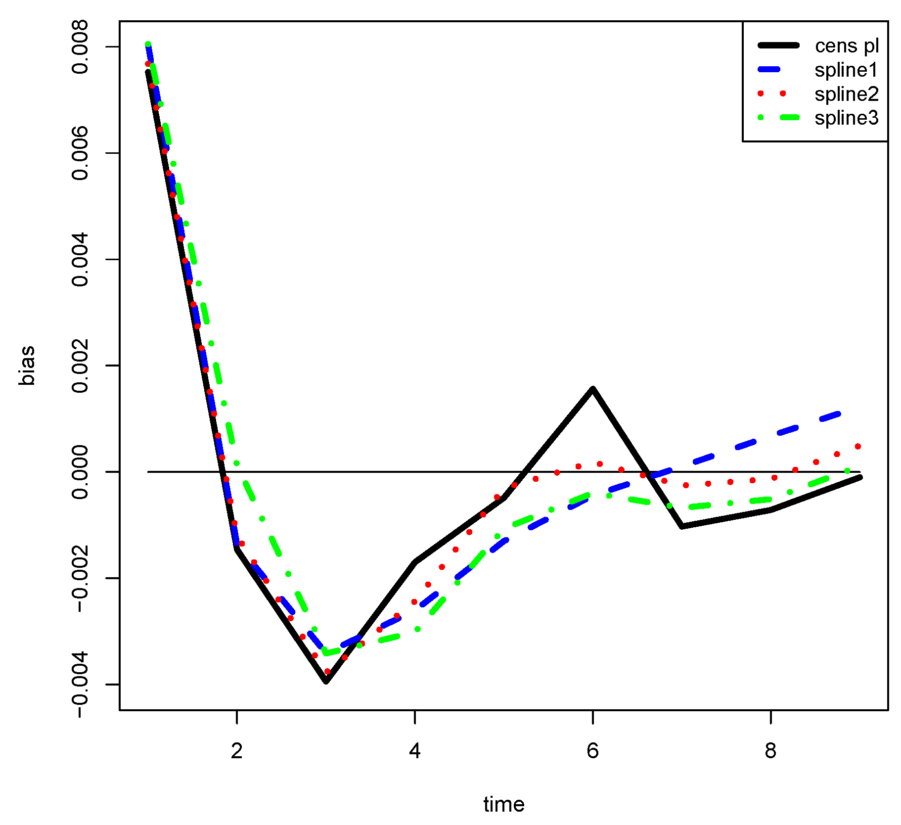
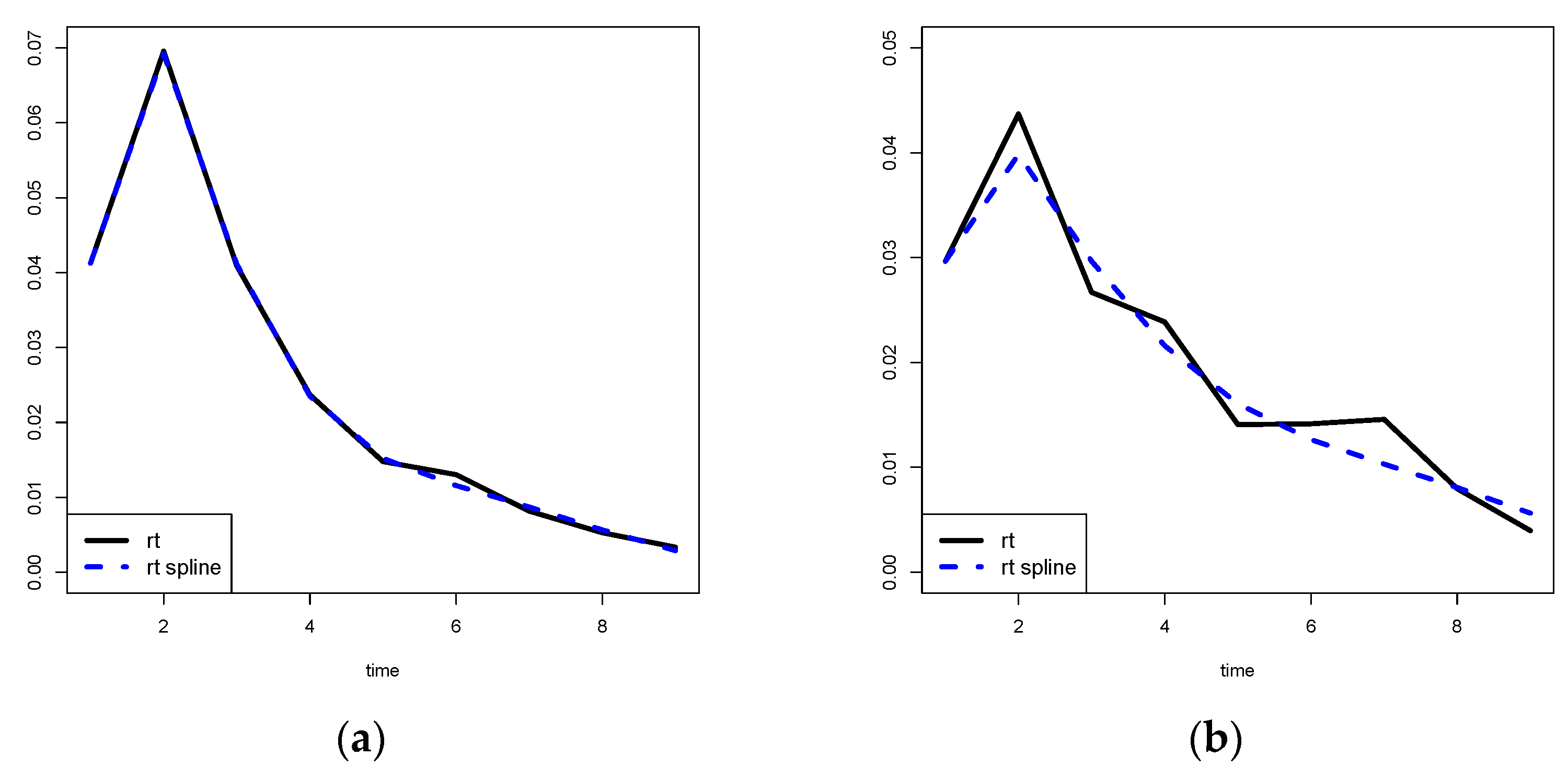
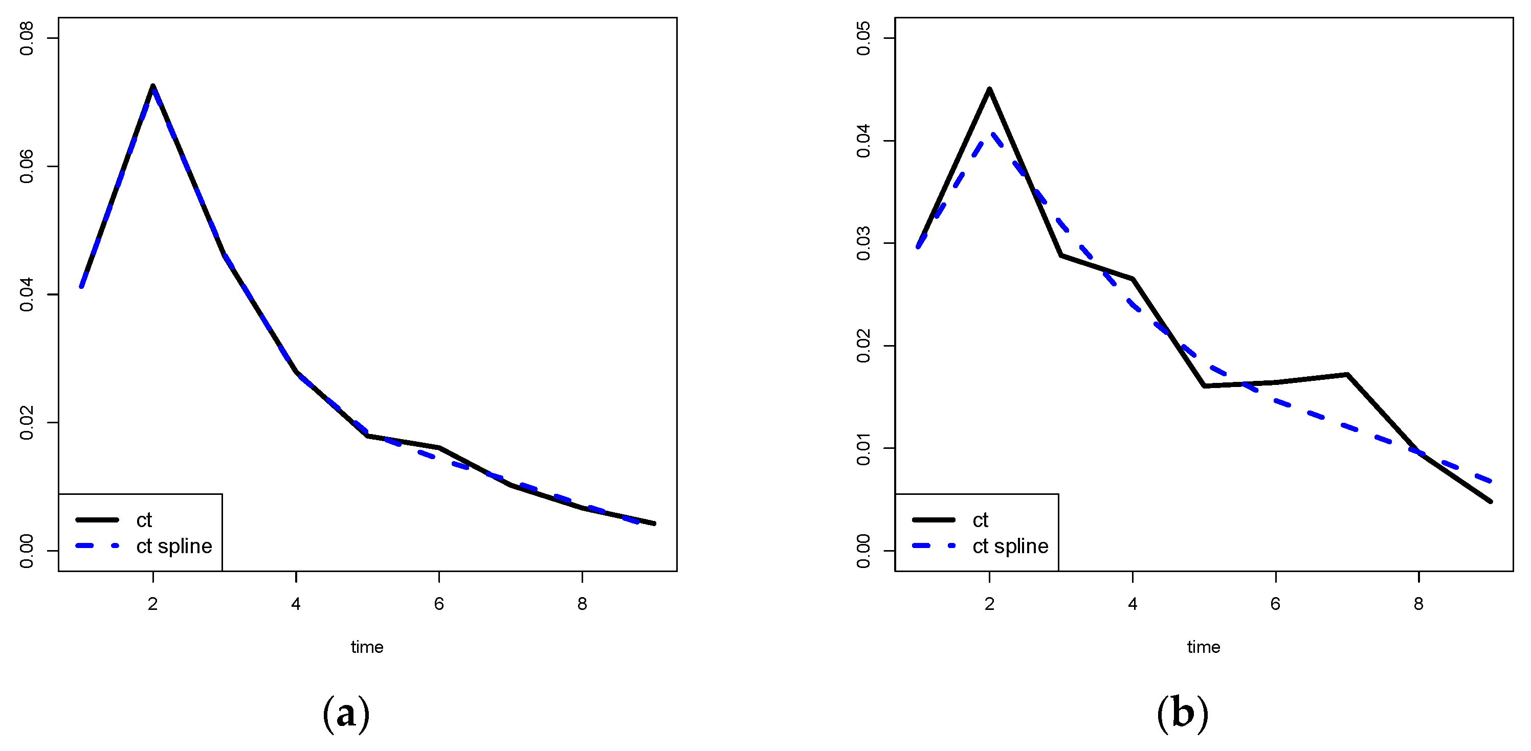
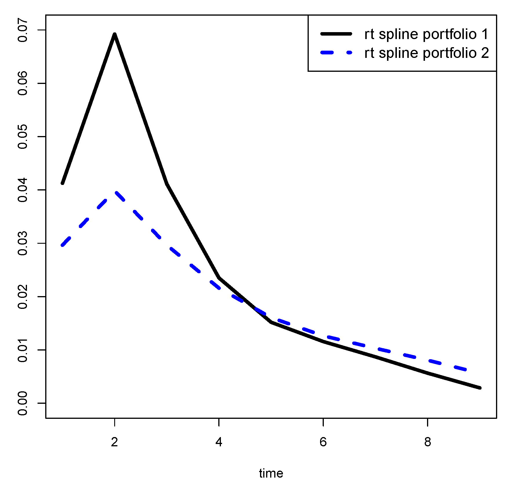
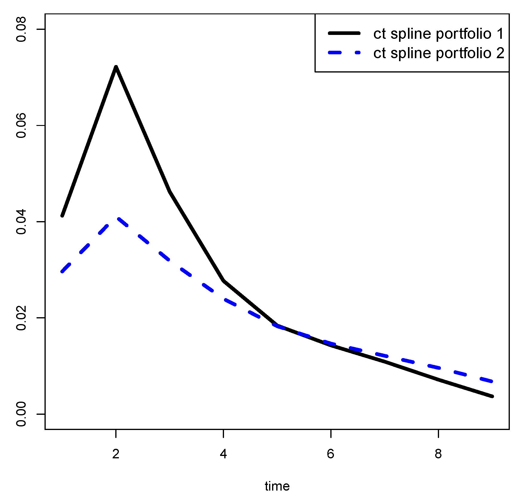
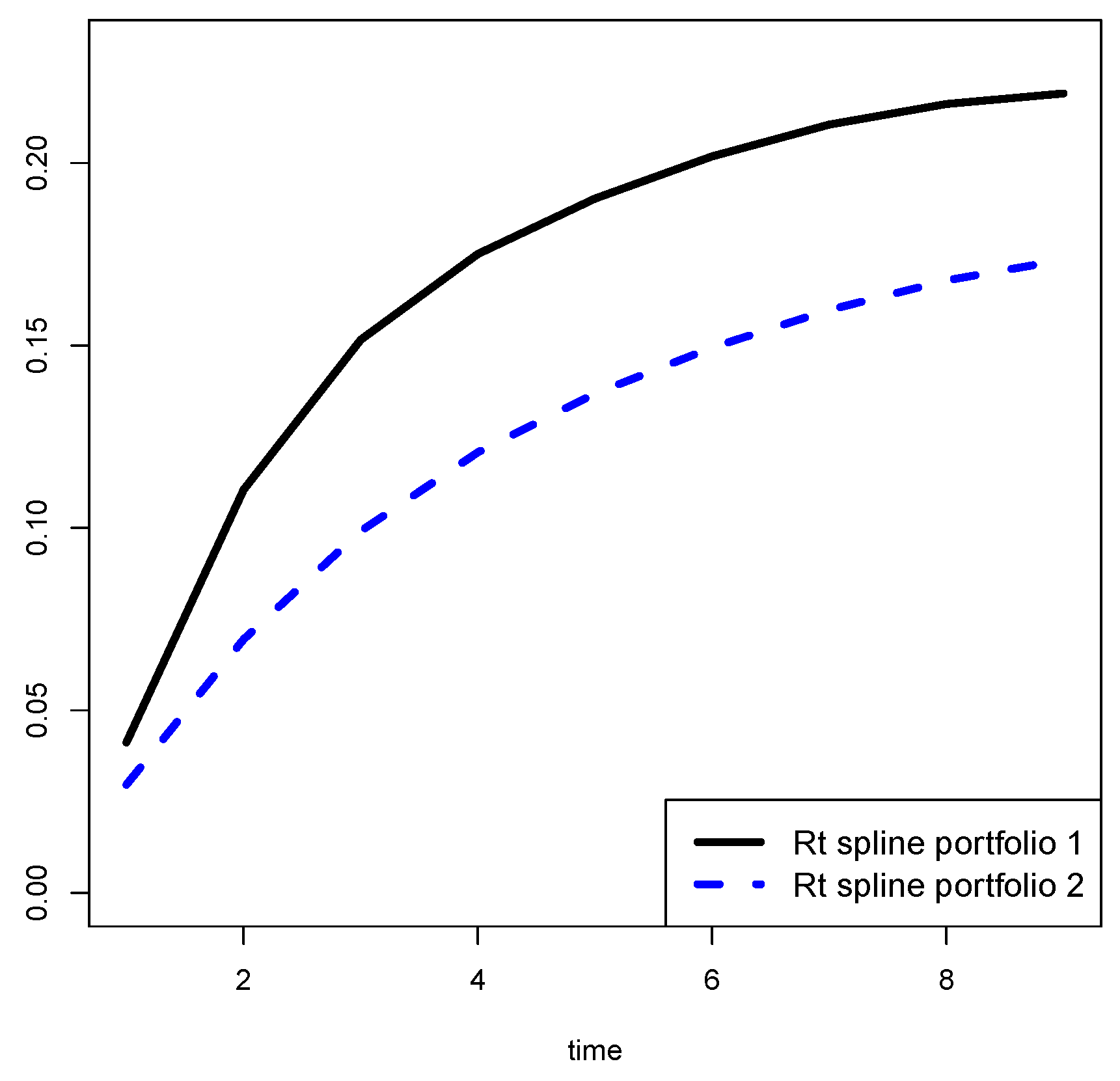
2.3. Spline Smoothing on the $c_t$s

In general, when we plot the $c_{k,t}$ (and the $r_{k,t}$), for $t=1,2,\dots ,T$, we expect to see a smooth curve. Then, it would be opportune to produce smoothed estimates of the $c_t$s.

To this end, first we note that the portfolio conditional recovery rate $c_t$ is a weighted average of the NPLs conditional recovery rates $c_{k,t}=\frac{p_{k,t}}{E_{k,t}}$

$$c_t=\frac{{{\displaystyle \sum }}_{k\in K_t}{p}_{k,t}}{{{\displaystyle \sum }}_{h\in K_t}{E}_{h,t}}=\frac{1}{{{\displaystyle \sum }}_{h\in K_t}{E}_{h,t}}{\displaystyle \sum }_{k\in K_t}\frac{p_{k,t}}{E_{k,t}}{E}_{k,t}=\frac{1}{{{\displaystyle \sum }}_{h\in K_t}{E}_{h,t}}{\displaystyle \sum }_{k\in K_t}{c}_{k,t}{E}_{k,t}$$

(11)

It follows that the $c_t$s minimizes the least squares loss.

$${\displaystyle \sum }_{t=1}^T{\displaystyle \sum }_{k\in K_t}{E}_{k,t}{\left(c_{k,t}-c_t\right)}^2$$

(12)

Our idea is to estimate the $c_t$s by using a non-parametric regression technique.

In particular, we propose to use penalized regression splines by minimizing the loss (spline 1)

$${\displaystyle \sum }_{t=1}^T{\displaystyle \sum }_{k\in K_t}{E}_{k,t}{\left(c_{k,t}-f\left(t\right)\right)}^2+\mathsf{\lambda }{\displaystyle \int }{\left[f^{″}\left(x\right)\right]}^{2}dx$$

(13)

where $f\left(t\right)$ is the “smoothed” version of $c_t$.

In practical applications, the choice of $\lambda$ is crucial, as large values reduce the variability of the estimator but increase its bias while small values reduce the bias but increase the variance. In our implementation, we use the R [37] package MGCV (mixed GAM computation vehicle with automatic smoothness estimation) [38]. The smoothing parameter is selected using the GCV (generalized cross-validation) criterion.

It is interesting to note that the loss (13) is equal to

$${\displaystyle \sum }_{t=1}^T{\displaystyle \sum }_{k\in K_t}{E}_{k,t}{\left(c_{k,t}-c_t\right)}^2+{\displaystyle \sum }_{t=1}^T{E}_t{\left(c_t-f\left(t\right)\right)}^2+\mathsf{\lambda }{\displaystyle \int }{\left[f^{″}\left(x\right)\right]}^{2}dx$$

(14)

It follows that the second addendum of (14) gives a loss equivalent to (13). We name this loss spline 2. Although the two losses are equivalent with respect to minimization, in our implementation they give different results because they are not equivalent with respect to the choice of $\lambda$.

Another possibility is given by the minimization of the loss (spline 3)

$${\displaystyle \sum }_{t=1}^T\frac{E_t^3}{s_t^2{\mathsf{\Sigma }}_{k\in K_t}{E}_{k,t}^2}{\left(c_t-f\left(t\right)\right)}^2+\mathsf{\lambda }{\displaystyle \int }{\left[f^{″}\left(x\right)\right]}^{2}dx$$

(15)

where $s_t^2$ is an estimate of the variance of the $c_t$s. It corresponds to weight the “observations” by the inverse of their variances.

3. Results

In this section, we apply our methodology to several datasets, some simulated (Section 3.1) and others real (Section 3.2).

3.1. Simulation Study

In Figure 1, we draw the recovery curve of an NPL portfolio, considering $T=9$ years of delay in payment from the default. The recovery curve is expressed both in terms of recovery rate $r_t$ (dashed blue line) and conditional recovery rate $c_t$ (solid black line) over the years.

Starting from the recovery curve in Figure 1, we generated 1000 portfolios each composed of 100 NPLs.

In each portfolio, the trajectory of the $k-th$ NPL has been generated as

$EA{D}_k$ ~ Gamma $\left(\mathrm{mean} =1000, \mathrm{s}.\mathrm{d}.=100\right)$;

$c_{k,t}$~ Beta $\left(\mathrm{mean} =c_t, \mathrm{s}.\mathrm{d}.=\sqrt{\frac{c_t\left(1-c_t\right)}{11}}\right)$.

An NPL has been censored at random with probability $0.4$.

The censoring started from the time interval $t$ ($>1$) with probability $\left(\begin{array}{c}7\\ t-2\end{array}\right){0.8}^{t-2}{\left(1-0.8\right)}^{9-t}$) [mean = 7.6]

Each random variable has been generated independently from the others.

We considered the following three estimators:

• “no cens”: the plain estimator applied to the data without censoring. This is our benchmark, i.e., the best estimator because it works on the complete data;
• “cens pl”: the product limit estimator applied to the censored data, i.e., our proposal;
• “cens del”: the plain estimator applied on the censored data deleting the NPLs having an incomplete trajectory, i.e., what practitioners frequently use.

The goodness in recovering the true $r_t$ curve has been measured in terms of:

• bias at time t: $\mathrm{mean}\left({\widehat{r}}_t-r_t\right)$;
• standard error at time t: $\sqrt{\mathrm{mean}\left({\left({\widehat{r}}_t-r_t\right)}^2\right)}$

All computations have been conducted in R [37].

In Figure 2, we show the bias in Figure 2a and the standard error in Figure 2b for each of the three estimators.

Examining the plot of the results in Figure 2b, we note that the standard errors decrease with time. This is due to the fact that the variance of the recovery rate of the simulated single loan decreases with time. Comparing the curves in Figure 2, we see that the lines corresponding to the “no cens” estimator (black solid line) and the “cens pl” estimator (blue dashed line) are overlapping at any time $t<7$ and with slight differences in the last years, for the effect of censoring. The line corresponding to the “cens del” estimator (red dotted line) is very different displaying a higher bias and standard error. This is due to the lack of information caused by the smaller number of loans considered, which is significant in the first years and less influential in the last years when the data are censored and the three estimators tend to collapse, as we can see in Figure 3 from the zoom of the tails of the previous plots.

On the same data, we also evaluated the performance of the three spline estimators proposed in Section 2.3 (colored dashed lines) in comparison with the “cens pl” estimator (black solid line). The results are depicted in Figure 4 and Figure 5. Figure 4 depicts the results in terms of bias and Figure 5 depicts the results in terms of standard error.

From the results of the experiment, we deduce that smoothing does not help in reducing the bias (see Figure 4), while it helps in reducing the standard error (see Figure 5).

In particular, splines 1 and 3 are better than spline 2. However, it is difficult to choose between the two because spline 3 performs better than spline 2 around $t=6$ but loses efficiency after $t=8$.

3.2. Application

We analyze a data set of Italian NPLs supplied by a specialized operator, doValue, active in Southern Europe in credit and real estate asset management services, mainly deriving from non-performing loans, on behalf of banks and investors.

We examine two portfolios of unsecured loans with different initial debt sizes: one portfolio of unsecured loans with an initial debt size between EUR $5000$ and $\mathrm{15,000} (5000<EA{D}_k<\mathrm{15,000})$ and one portfolio of unsecured loans with an initial debt size between EUR 100,000 and 250,000 $(\mathrm{100,000}<EA{D}_k<\mathrm{250,000})$. The years of acceptance by the operator are 2006, 2007, 2008, 2009, and 2010, and data are available until 2015.

In particular, the description of the two portfolios is summarized in

Table 10. Descriptive stats of the two portfolios.

	Portfolio 1	Portfolio 2
K	3386.00	3084.00
Min	5004.62	100,027.45
1st Qu.	7262.03	118,246.80
Median	9796.60	144,541.51
Mean	9848.48	152,075.82
3rd Qu.	12,376.21	178,418.88
Max	15,000.00	249,205.54
sd	2902.53	39,188.61

.

Figure 6 describes the distribution of the exposure at default (EAD) in Portfolio 1 and Portfolio 2 in Figure 6a,b, respectively.

From Table 10 and the histograms in Figure 6, we see that the two portfolios are quite large, with an EAD distribution that is substantially uniform for portfolio 1. The EAD distribution is highly skewed for portfolio 2. This is not strange because the loans in portfolio 1 are on average more than 15 times larger.

We consider as starting time ($t=0$) the year of acceptance, rather than the exact time of default, because this is the moment in which the operator starts the recovery procedure. We followed the recovery history for 9 years. Only about 14% of the records are complete, i.e., the ones accepted in 2006.

The plot of the results in terms of recovery rate at time $t$($r_t$) is in Figure 7. In particular, the black solid line represents the non-smoothed recovery curve, and the blue dashed line represents the smoothed recovery curve, both in terms of recovery rate at time t ($r_t$), for portfolio 1 in Figure 7a and for portfolio 2 in Figure 7b. In the same way, Figure 8 represents the results in terms of conditional recovery rate at time t ($c_t$).

From Figure 7 and Figure 8, we see that, as expected, the highest values of the recovery are at the beginning of the observation period, meaning that the procedures put in place by specialized operators obtain a significant effect as soon as the debt is processed, while as time passes, the recovery tends to decrease. It is interesting to note that the highest recovery is obtained in $t=2$ rather than $t=1$. This is probably because the recovery procedures that the operator implements require a certain amount of time to reach their maximum efficiency. It is important to say that in order to “learn” from the data the peak in $t=2$, we applied the regression splines only in the range $t=2:9$.

To compare the results, it is useful to draw the curves of both portfolios on a single plot. In Figure 9, Figure 10 and Figure 11, we represent the smoothed recovery curves for portfolio 1 with a black solid line and for portfolio 2 with a blue dashed line in terms, respectively, of recovery rate at time t ($r_t$), conditional recovery rate at time t ($c_t$), and recovery rate until time t ($R_t$).

It appears, in Figure 9 and Figure 10, that in the first years, the recovery is greater for the portfolio with smaller credits and vice versa. Probably, this is because taking charge with specialized operators has at the beginning greater effect on those who have to return lower amounts, and after a certain number of years, the operator puts more effort into recovering larger amounts. Anyway, Figure 11 shows that the overall recovery is higher for the portfolio with lower credits in the entire period.

Finally, it is interesting to compare our results with those obtained in [29], where the authors analyzed a portfolio with a smaller number of defaulted loans, 374, belonging to a Portuguese bank. They compute for each loan the conditional recovery rates and then aggregate them as an unweighted or weighted average, taking into account the size of the loans. In the paper, they first report the non-smoothed, unweighted average conditional recovery curve. It shows a shape similar to our curves but without the peak at the beginning. They also report the non-smoothed curves of the recovery rate until time t is computed using the weighted and unweighted approach. The main difference is in the height; their weighted curve is dominated by the unweighted curve, and it is always more than 30–40% greater than ours. This is due to several reasons: different countries, different time frames, etc. Among them is the fact that our sample consists only of unsecured loans that have been sold.

4. Discussion

According to the objective of this paper, we propose a kind of measurement that takes into consideration both the recovery rate and the time to liquidate. In our opinion, an efficient way to do that is to measure a recovery curve in terms of recovery rate until time $t$, so as to observe the behavior of the recovery rate during that time.

In doing that, we have to face the problem of censored data, and we suggest using a method of measuring performances that allows not only to measure jointly the recovery rate and the time to liquidate but also to deal with censored data. This method is based on an algorithm that is usually used in the construction of actuarial mortality tables and survival curves. The estimation method has been improved by smoothing the curve by using regression splines. The method has been tested on simulated and real data.

In our opinion, the present study is promising and can be extended in several directions.

Firstly, by eliminating some of the current limits. Our technique assumes that the recovery rate is always between 0 and 1 while we know that in real cases this is not necessarily true. Another assumption is that the data can be incomplete only through a censoring process, while other kinds of data loss may occur. Those are limits to the methodology; however, there are also limits to the availability of the data. As reported in [29], as bank loans are private instruments, few data on loan losses are publicly available.

Secondly, by extending the current approach to different objectives. As an example, it would be interesting to classify a set of NPLs on the basis of their recovery curves. Another example arises from the application reported in the study. We have seen how the recovery curve depends on the size of the loan; it would also be interesting to study how it depends on other characteristics of the loan.

References

1. Resti, A.; Sironi, A. Risk Management and Shareholders’ Value in Banking; John Wiley & Sons: Hoboken, NJ, USA, 2007. [Google Scholar]
2. Basel Committee on Banking Supervision. The Internal Ratings-Based Approach; Bank for International Settlements: Basel, Switzerland, 2001; Available online: https://www.bis.org/publ/bcbsca05.pdf (accessed on 30 January 2023).
3. Basel Committee on Banking Supervision. Principles for Sound Liquidity Risk Management and Supervision; Bank for International Settlements: Basel, Switzerland, 2008; Available online: http://www.bis.org/publ/bcbs144.pdf (accessed on 30 January 2023).
4. Basel Committee on Banking Supervision. Basel III: Finalising Post-Crisis Reforms; Bank for International Settlements: Basel, Switzerland, 2017; Available online: https://www.bis.org/bcbs/publ/d524.pdf (accessed on 30 January 2023).
5. European Banking Authority. Guidelines on PD Estimation, LGD Estimation and the Treatment of Defaulted Exposure. 2017. Available online: https://www.eba.europa.eu/sites/default/documents/files/documents/10180/2033363/6b062012-45d6-4655-af04-801d26493ed0/Guidelines%20on%20PD%20and%20LGD%20estimation%20%28EBA-GL-2017-16%29.pdf?retry=1 (accessed on 30 January 2023).
6. Hastie, T.; Tibshirani, R.; Friedman, J. The Elements of Statistical Learning, 2nd ed.; Springer Series in Statistics; Springer: New York, NY, USA, 2009. [Google Scholar]
7. Yao, X.; Crook, J.; Andreeva, G. Support Vector Regression for Loss Given Default Modelling. Eur. J. Oper. Res. 2015, 240, 528–538. [Google Scholar] [CrossRef]
8. Ye, H.; Bellotti, A. Modelling Recovery Rates for Non-performing Loans. Risks 2019, 7, 19. [Google Scholar] [CrossRef]
9. Bellotti, A.; Brigo, D.; Gambetti, P.; Vrins, F. Forecasting recovery rates on non-performing loans with machine learning. Int. J. Forecast. 2021, 37, 428–444. [Google Scholar] [CrossRef]
10. Cheng, D.; Cirillo, P. A reinforced urn process modeling of recovery rates and recovery times. J. Bank. Financ. 2018, 96, 1–17. [Google Scholar] [CrossRef]
11. Gambetti, P.; Roccazzella, F.; Vrins, F. Meta-Learning Approaches for Recovery Rate Prediction. Risks 2022, 10, 124. [Google Scholar] [CrossRef]
12. Kaposty, F.; Kriebel, J.; Löderbusch, M. Predicting loss given default in leasing: A closer look at models and variable selection. Int. J. Forecast. 2020, 36, 248–266. [Google Scholar] [CrossRef]
13. Min, A.; Scherer, M.; Schischke, A.; Zagst, R. Modeling Recovery Rates of Small and Medium-Sized Entities in the US. Mathematics 2020, 8, 1856. [Google Scholar] [CrossRef]
14. Loterman, G.; Brown, I.; Martens, D.; Mues, C.; Baesens, B. Benchmarking regression algorithms for loss given default modeling. Int. J. Forecast. 2012, 28, 161–170. [Google Scholar] [CrossRef]
15. Qi, M.; Zhao, X. Comparison of modeling methods for loss given default. J. Bank. Financ. 2011, 35, 2842–2855. [Google Scholar] [CrossRef]
16. Krüger, S.; Rösch, D. Downturn LGD Modeling using Quantile Regression. J. Bank. Financ. 2017, 79, 42–56. [Google Scholar] [CrossRef]
17. Gostkowski, M.; Gajowniczek, K. Weighted Quantile Regression Forests for Bimodal Distribution Modeling: A Loss Given Default Case. Entropy 2020, 22, 545. [Google Scholar] [CrossRef] [PubMed]
18. Altman, I.E.; Kalotay, A.E. Ultimate Recovery Mixtures. J. Bank. Financ. 2014, 40, 116–129. [Google Scholar] [CrossRef]
19. Betz, J.; Kellner, R.; Rösch, D. Systematic Effects among Loss Given Defaults and their Implications on Downturn Estimation. Eur. J. Oper. Res. 2018, 271, 1113–1144. [Google Scholar] [CrossRef]
20. Calabrese, R. Downturn loss given default: Mixture distribution estimation. Eur. J. Oper. Res. 2014, 237, 271–277. [Google Scholar] [CrossRef]
21. Kalotay, A.E.; Altman, I.E. Intertemporal Forecasts of Defaulted Bond Recoveries and Portfolio Losses. Rev. Financ. 2017, 21, 433–463. [Google Scholar] [CrossRef]
22. Tomarchio, S.D.; Punzo, A. Modelling the Loss Given Default Distribution via a Family of Zero-and-one Inflated Mixture Models. J. R. Stat. Soc. Ser. A 2019, 182, 1247–1266. [Google Scholar] [CrossRef]
23. Bellotti, T.; Crook, J. Loss given default models incorporating macroeconomic variables for credit cards. Int. J. Forecast. 2012, 28, 171–182. [Google Scholar] [CrossRef]
24. Bijak, K.; Thomas, L. Modelling LGD for unsecured retail loans using Bayesian methods. J. Oper. Res. Soc. 2015, 66, 342–352. [Google Scholar] [CrossRef]
25. Sun, H.S.; Jin, Z. Estimating credit risk parameters using ensemble learning methods: An empirical study on loss given default. J. Credit Risk 2016, 12, 43–69. [Google Scholar] [CrossRef]
26. Tobback, E.; Martens, D.; Van Gestel, T.; Baesens, B. Forecasting Loss Given Default models: Impact of account characteristics and the macroeconomic state. J. Oper. Res. Soc. 2014, 65, 376–392. [Google Scholar] [CrossRef] [Green Version]
27. Devjak, S. Modeling of Cash Flows from Nonperforming Loans in a Commercial Bank. Naše Gospod. Our Econ. 2018, 64, 3–9. [Google Scholar] [CrossRef]
28. Betz, J.; Kellner, R.; Rösch, D. Time matters: How default resolution times impact final loss rates. J. R. Stat. Soc. Ser. C 2021, 70, 619–644. [Google Scholar] [CrossRef]
29. Dermine, J.; Neto de Carvalho, C. Bank loan losses-given-default: A case study. J. Bank. Financ. 2006, 30, 1219–1243. [Google Scholar] [CrossRef]
30. Witzany, J.; Rychnovsky, M.; Charamza, P. Survival Analysis in LGD Modeling. Eur. Financ. Account. J. 2012, 7, 6–27. [Google Scholar] [CrossRef]
31. Zhang, J.; Thomas, L.C. Comparisons of linear regression and survival analysis using single and mixture distributions approaches in modelling LGD. Int. J. Forecast. 2012, 28, 204–215. [Google Scholar] [CrossRef]
32. Kalbfleisch, J.D.; Prentice, R.L. The Statistical Analysis Failure Time Data, 2nd ed.; John Wiley & Sons: Hoboken, NJ, USA, 2002. [Google Scholar]
33. Altman, E.I. Measuring Corporate Bond Mortality and Performance. J. Financ. 1989, 44, 909–922. [Google Scholar] [CrossRef]
34. Rocci, R.; Carleo, A.; Staffa, M.S. Estimating Recovery Curve for NPLs. In Mathematical and Statistical Methods for Actuarial Sciences and Finance. MAF 2022; Corazza, M., Perna, C., Pizzi, C., Sibillo, M., Eds.; Springer: Cham, Switzerland, 2022; pp. 397–403. [Google Scholar] [CrossRef]
35. Rocci, R.; Carleo, A.; Staffa, M.S. Estimating recovery rate and time to liquidate for NPLs. In Working Paper n. 16, Università degli Studi Roma Tre, Collana del Dipartimento di Economia Aziendale; Università degli Studi Roma Tre: Rome, Italy, 2021; Available online: https://economiaziendale.uniroma3.it/wp-content/uploads/sites/9/file_locked/2021/12/WP16-Carleo.pdf (accessed on 30 January 2023).
36. Basel Committee on Banking Supervision. Guidance on Paragraph 468 of the Framework Document; Bank for International Settlements: Basel, Switzerland, 2005; Available online: http://www.bis.org/publ/bcbs115.pdf (accessed on 30 January 2023).
37. R Core Team. R: A Language and Environment for Statistical Computing; R Foundation for Statistical Computing: Vienna, Austria, 2022; Available online: https://www.R-project.org/ (accessed on 30 January 2023).
38. Wood, S. Generalized Additive Models: An Introduction with R, 2nd ed.; Chapman and Hall/CRC: Boca Raton, FL, USA, 2017. [Google Scholar] [CrossRef] [Green Version]
Figure 1. Recovery curve with T = 9 , expressed both in terms of recovery rate ( r t ) and conditional recovery rate ( c t ).
Computation 11 00029 g001
Figure 2. Bias (a) and standard (b) error for each of the three estimators.
Computation 11 00029 g002
Figure 3. Zoom of the tail of the plot in Figure 2. (a) Bias and (b) standard.
Computation 11 00029 g003
Figure 4. Bias for each of the three splines of “cens pl” estimator.
Computation 11 00029 g004
Figure 5. Standard errors for each of the three splines of “cens pl” estimators.
Computation 11 00029 g005
Figure 6. EAD distribution in (a) portfolio 1 and (b) portfolio 2.
Computation 11 00029 g006
Figure 7. Recovery rate at time t   ( r t ) smoothed and non-smoothed for (a) portfolio 1; and (b) portfolio 2.
Computation 11 00029 g007
Figure 8. Conditional recovery rate at time t   ( c t ) smoothed and non-smoothed for (a) portfolio 1; and (b) portfolio 2.
Computation 11 00029 g008
Figure 9. Comparison of recovery curve in term of r t for portfolio 1 and portfolio 2.
Computation 11 00029 g009
Figure 10. Comparison of recovery curve in term of c t for portfolio 1 and portfolio 2.
Computation 11 00029 g010
Figure 11. Comparison of recovery curve in term of R t for portfolio 1 and portfolio 2.
Computation 11 00029 g011