An Approach to Implementing High-Performance Computing for Problem Solving in Workflow-Based Energy Infrastructure Resilience Studies

Abstract

Implementing high-performance computing (HPC) to solve problems in energy infrastructure resilience research in a heterogeneous environment based on an in-memory data grid (IMDG) presents a challenge to workflow management systems. Large-scale energy infrastructure research needs multi-variant planning and tools to allocate and dispatch distributed computing resources that pool together to let applications share data, taking into account the subject domain specificity, resource characteristics, and quotas for resource use. To that end, we propose an approach to implement HPC-based resilience analysis using our Orlando Tools (OT) framework. To dynamically scale computing resources, we provide their integration with the relevant software, identifying key application parameters that can have a significant impact on the amount of data processed and the amount of resources required. We automate the startup of the IMDG cluster to execute workflows. To demonstrate the advantage of our solution, we apply it to evaluate the resilience of the existing energy infrastructure model. Compared to similar approaches, our solution allows us to investigate large infrastructures by modeling multiple simultaneous failures of different types of elements down to the number of network elements. In terms of task and resource utilization efficiency, we achieve almost linear speedup as the number of nodes of each resource increases.

1. Introduction

The economy and society’s welfare are now highly dependent on the resilience of critical infrastructures to various disturbances [1]. Energy infrastructure is among the vital infrastructures because it supports the functioning of other dependent infrastructures. Therefore, given the large scale of this complex and multi-layered infrastructure, researching its resilience is undoubtedly challenging. Many experts in the field pay special attention to it [2,3]. In particular, the following key characteristics of energy infrastructure resilience are identified qualitatively: anticipation, resistance, adaptation, and recovery. The essence of anticipation is predicting disturbance events and taking preventive actions. Resistance is defined as the ability of an energy infrastructure to absorb the impact of disturbance and mitigate its consequences with minimal effort. The adaptation reflects how an energy infrastructure can self-organize to prevent system performance degradation and overcome disturbances without restoration activities. Finally, the recovery shows the ability to restore the system functioning to its original operating level.

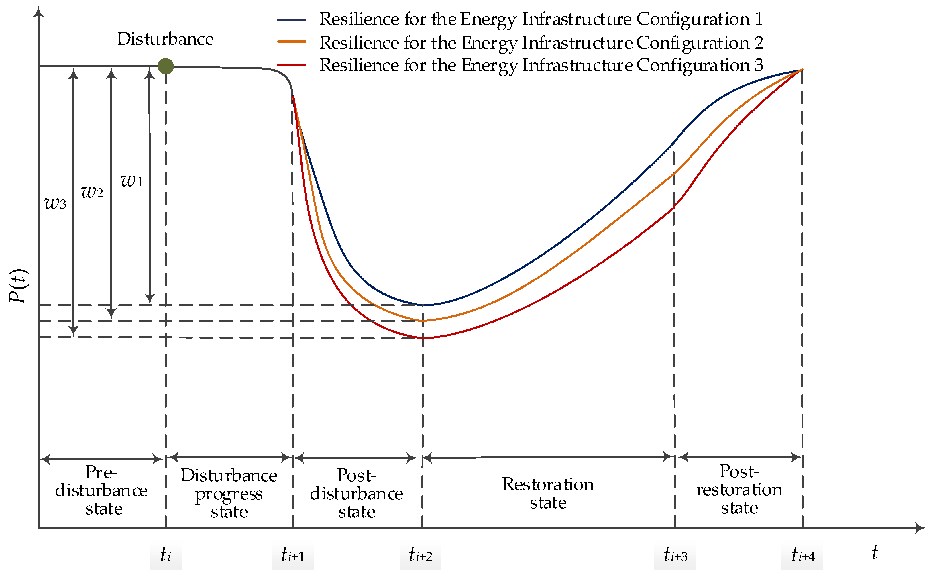
To assess the resilience of energy infrastructures, it is necessary to investigate the changes between the states of the energy infrastructure before, during, and after the disturbance.

In general, such changes are represented by resilience curves [4]. These curves show the performance evolutions over time under a disturbance scenario for different energy infrastructure configurations (Figure 1). Each curve reflects the following states:

Figure 1. Resilience curves.

• Pre-disturbance state ($t<t_j$) that shows the stable performance $P\left(t\right)$;
• Disturbance progress state ($t\in \left[t_j,t_{j+1}\right]$) showing the occurrence of a disturbance and the eventual performance degradation $P\left(t\right)$;
• Post-disturbance degraded state ($t\in \left[t_{j+1},t_{j+2}\right]$) characterized by a rapid performance degradation $P\left(t\right)$ from $t_{j+1}$;
• Restoration state ($t\in \left[t_{j+2},t_{j+3}\right]$) when the performance $P\left(t\right)$ gradually increases from $t_{j+2}$ to $t_{j+3}$, and the energy infrastructure reaches a stable condition;
• Post-restoration state ($t\in \left[t_{j+3},t_{j+4}\right]$), in which the performance $P\left(t\right)$ reaches a level comparable to that before the disturbance.

Puline et al. [4] introduce metrics to quantify resilience based on the shape and size of curve segments. Let a disturbance scenario contain $n_p$ periods and the vector $s^{\tau }=\left(s_1^{\tau },s_2^{\tau },\dots ,s_m^{\tau }\right)$ describe the state of the energy infrastructure at the period $\tau \in \overline{1,n_p}$.

The performance measure $y\left(S,\tau \right):s^{\tau }\to \mathrm{R}$ maps the energy infrastructure state $s^{\tau }$ from the set $S=\left\{s^1,s^2,\dots ,s^{n_p}\right\}$ to a scalar value. The summary metric $w\left(S,\left[a,b\right]\right):\left(y\left({S,i}_1\right),y\left(S,i_2\right),\dots ,y\left({S,i}_k\right)\right)\to \mathrm{R}$, where $a=i_1$, $b=i_k$, $i_1<i_2<\dots <i_k$, $i_1,i_2,\dots ,i_k\in \overline{1,n_p}$, maps a curve segment to a scalar value. The following data sources can be used to plot resilience curves: retrospective information, natural experiment results, simulation and analytical modeling, artificial neural networks, network flow methods, etc.

Within our study, we consider one of the fundamental metrics of energy infrastructure resilience called vulnerability. A vulnerability is studied within a global vulnerability analysis (GVA) [5]. Such an analysis aims to evaluate the extent to which the performance degradation of the energy infrastructure configuration depends on the disturbance parameters [6]. GVA is based on modeling a series of disturbance scenarios with a large number of failed elements.

An energy infrastructure configuration includes the following entities: energy facility descriptions and data about the natural, climatic, technological, social, and economic conditions for the operation of these facilities. We can compare different energy infrastructure configurations in terms of vulnerability based on analyzing the performance degradation that is due to a disturbance. The steeper and deeper the slope of the resilience curve segment in the resistance and absorption states for a specific configuration, the more vulnerable this configuration is to disturbance parameters. For example, the curve segment from $t_i$ to $t_{i+2}$ in Figure 1 reflects the resistance state in the form of a sharp degradation in the energy infrastructure performance $P\left(t\right)$. The metrics $w_1\left(S,\left[t_i,t_{i+2}\right]\right)$, $w_2\left(S,\left[t_i,t_{i+2}\right]\right)$, and $w_3\left(S,\left[t_i,t_{i+2}\right]\right)$ equal to $P\left(t_i\right)-P\left(t_{i+2}\right)$ show the vulnerability of the energy infrastructure due to the performance degradation in the two states above for Configurations 1, 2, and 3, respectively. In this example, $w_1<w_2<w_3$. Therefore, Energy Infrastructure Configuration 1 is the least vulnerable.

Researchers involved in implementing GVA are faced with its high computational complexity. It is necessary to create sets of possible disturbance scenarios by varying their parameters for each energy infrastructure configuration. However, the problem-solving process is well parallelized into many independent subtasks. Each subtask investigates the vulnerability of a particular energy infrastructure configuration to a set of disturbance scenarios. In this context, we implement GVA based on the integrated use of HPC, a modular approach to application software development, parameter sweep computations, and IMDG technology.

The rest of the paper is structured as follows. Section 2 briefly reviews approaches for implementing high-performance computing and scientific applications in power system research. Section 3 discusses the main aspects of performing GVA. Section 4 presents the workflow-based distributed scientific application that implements the proposed approach. Section 5 discusses the results of computational experiments. Finally, Section 6 concludes the paper.

2. Related Work

This section introduces the most appropriate approaches to implementing the following three aspects of computing organization that drive our problem solving:

• HPC for solving similar problems in general;
• IMDG technology to increase the efficiency of storing and processing the computation results in comparison with traditional data storage systems;
• Capabilities of software systems to create and execute the required problem-solving workflows.

2.1. High-Performance Computing Implementations

According to an analysis of the available literature describing the software and hardware to study power systems, the solutions developed in this research field generally focuses on solving specific problems with predefined dimensions [7]. The applied software adapts to the capabilities of the available software and hardware of computing systems [8]. This approach dramatically simplifies software development. However, the problem specification capabilities and increasing its dimension are usually limited. Moreover, it is impossible to distinguish a unified way to implement parallel or distributed computing for a wide range of problems. At the same time, solving many tasks requires capabilities in computing environments that are dynamically determined and changed for the problem dimensions and algorithms used.

We distinguish the following three general approaches:

• Developing multi-threaded programs for systems with shared memory based on the OpenMP or other standards [8,9,10]. This approach uses high-level tools for developing and debugging parallel programs. However, the structure of the programs can have a high complexity. As a rule, this approach allows us to solve problems of relatively low dimensionality. Otherwise, it is necessary to use special supercomputers with shared memory [8] or implement computations using the capabilities of other approaches.
• Implementing MPI programs [9,10]. This approach focuses on homogeneous computing resources and allows us to solve problems of any complexity, depending on the number of resources. It is characterized by more complex program structures and low-level tools for software development and debugging.
• Creating distributed applications for grid and cloud computing [11]. There is a large spectrum of tools for implementing distributed computing that provide different levels of software for development, debugging, and usage by both developers and end-users [12]. Undoubtedly, this approach can solve problems of high dimensions and ensure computational scalability. However, within such an approach, the challenge is allocating and balancing resources with different computational characteristics.

To solve the problems related to GVA, we based our study on the third approach using the capabilities of the first approach to implement parallel computing. In addition, we use the IMDG technology to speed up data processing.

2.2. IMDG Tools

IMDG-based data storage systems have an undeniable advantage in the data processing speed over traditional databases [13]. Moreover, a large spectrum of tools to support the IMDG technology on the HPC resources is available [14,15]. Each tool is a middleware to support the distributed processing of large data sets. Hazelcast 5.3.2 [16], Infinispan 14.0.7 [17], and Apache Ignite 2.15.0 [18] are the most popular freely distributed IMDG middleware for workflow-based and job-flow-based scientific applications with similar functionality and performance. They support client APIs on Java SE 17, C++ (ISO/IEC 14882:2020), and Python 3.12.0. End-users can use them to create IMDG clusters with distributed key/value caches. Each can have a processing advantage for a particular scenario and data set.

The Hazelcast platform is a real-time software for dynamic data operations. It integrates high-performance stream processing with fast data storage [19]. Some Hazelcast components are distributed under the Hazelcast Community License Agreement version 1.0.

Infinispan is the IMDG tool that provides flexible deployment options and reliable means to store, manage, and process data [20]. It supports and distributes key/value data on scalable IMDG clusters with high availability and fault tolerance. Infinispan is available under the Apache License 2.0.

Apache Ignite is a full-featured, decentralized transactional key-value database with a convenient and easy-to-use interface for real-time operation of large-scale data, including asynchronous in-memory computing [21]. It supports a long-term memory architecture with an in-memory and on-disk big data accelerator for data, computation, service, and streaming grids.

Apache Ignite is an open-source product under the Apache License 2.0. Unlike Hazelcast, the full functionality of Apache Ignite and Infinispan is free.

Within the SQL grid, Apache Ignite provides the operation with a horizontally scalable and fault-tolerant distributed SQL database that is highly ANSI-99 standard compliant. Hazelcast and Infinispan support similar SQL queries with exceptions.

In addition, to solve our problem, the IMDG middleware deployment on the computational nodes needs to be provisioned dynamically during the workflow execution. For Hazelcast and Infinispan, this key requirement is a time-consuming process. Typically, the Hazelcast and Infinispan end-users first deploy a cluster and only then run data processing tasks on the nodes of the deployed cluster. It was shown in various IMDG-based power system studies [22,23,24]. From this point of view, Apache Ignite is undoubtedly preferable.

Apache Ignite implements a methodology to determine the number of IMDG cluster nodes based on the projected amount of memory required to process data [25]. A similar technique was developed for Infinispan. However, Apache Ignite additionally considers the memory overheads of data storage and disk utilization. Hazelcast only provides examples that can be extrapolated for specific workloads.

We have successfully tested the above-listed advantages of Apache Ignite in practice in our preliminary studies [26] using the OT framework 2.0 [27]. Other researchers have also reported good results in energy system studies using Apache Ignite [28].

2.3. Workflow Management Systems

Apache Ignite, like Hazelcast, Infinispan, etc., does not support scheduling flows of data processing tasks. Therefore, additional tools are required for data decomposition, aggregation, pre-processing, task scheduling, resource allocation, and load balancing among the IMDG cluster nodes. If the set of data processing operations in a specific logical sequence correlates with the concept of a scientific workflow, the Workflow Management System (WMS) is best suited for scheduling.

A scientific workflow is a specialized form of a graph that describes processes and their dependencies used for data collection, data preparation, analytics, modeling, and simulation. It represents the business logic of a subject domain in applying subject-oriented data and software (a set of applied modules) for solving problems in this domain. WMS is a software tool that partially automates specifying, managing, and executing a scientific workflow according to its information and computation structure. A directed acyclic graph (DAG) is often used to specify a scientific workflow. In general, the DAG vertices and edges correspondingly represent the applied software modules and data flows between them.

The following WMSs are well-known, supported, developed, and widely used in practice: Uniform Interface to Computing Resources (UNICORE) 6 [29], Directed Acyclic Graph Manager (DAGMan) 10.9.0 [30], Pegasus 5.0 [31], HyperFlow 1.6.0 [32], Workflow-as-a-Service Cloud Platform (WaaSCP) [33], Galaxy 23.1 [34], and OT.

UNICORE, DAGMan, Pegasus, and OT are at the forefront of traditional workflow management. They are based on a modular approach to creating and using workflows. In the computing process, the general problem is divided into a set of tasks, generally represented by DAG. UNICORE and OT also provide additional control elements of branches and loops in workflows to support the non-DAG workflow representation.

Complex support of Web services is an actual direction of modern WSCs. The use of Web services greatly expands the computational capabilities of workflow-based applications. Web service-enabled WMSs allow us to flexibly and dynamically integrate various workflows created by different developers through the data and computation control in workflow execution. HyperFlow, WaaS Cloud Platform, Galaxy, and OT are successfully developing in this direction.

For scientific applications focused on solving various classes of problems in the field of environmental monitoring, integration with geographic information systems through specialized Web processing services (WPSs) is of particular importance. Representative examples of projects aimed at creating and using such applications are the GeoJModel-Builder (GJMB) 2.0 [35] and Business Process Execution Language (BPEL) Designer Project (DP) 1.1.3 [36]. GJMB and BPEL DP belong to the class of WMSs. GJMB is a framework for managing and coordinating geospatial sensors, data, and applied software in a workflow-based environment. BPEL DP implements the integration of the geoscience services and WPSs through the use of BPEL-based workflows.

The key capabilities of WMS, which are particularly important from the point of view of our study, are summarized in Table 1. The systems under consideration use XML-like or scripting languages for the workflow description. Support for branches, loops, and recursions in a workflow allows us to organize computing more flexibly if necessary. OT provides such support in full. An additional advantage of UNICORE, DAGMan, Pegasus, HyperFlow, Galaxy, GJMB, and OT is the ability to include system operations in the workflow structure. Such operations include pre- and post-processing of data, monitoring the computing environment, interaction with components of local resource managers, etc. HyperFlow, WaaSCP, Galaxy, GJMB, BPEL DP, and OT support Web services. Moreover, GJMB, BPEL DP, and OT support WPSs.

Table 1. WMS capabilities for supporting.

WMS	Workflow Description Language	Support for Branch/Loop/Recursion in Workflow	Support for System Operations in Workflow	Web Service Support	WPS Support
UNICORE	XML-like	+/+/−	+	+	−
DAGMan	Script-like	−/−/−	+	−	−
Pegasus	XML-like	−/−/−	+	−	−
HyperFlow	JavaScript, JSON	−/−/−	+	+	−
WaaSCP	XML-like	−/−/−	−	+	−
Galaxy	XML-like	−/+/−	+	+	−
GJMB	XML-like	−/−/−	+	+	+
BPEL DP	BPEL	+/+/−	−	+	+
OT	XML-like	+/+/+	+	+	+

Table 2 shows the capabilities of the WMSs to support parallel and distributed computing within the execution of workflows. The task level means that the tasks determined by the workflow structure are executed on the independent computing nodes. At the data level, a data set is divided into subsets. Each subset is processed on a separate computing node by all or part of the applied software modules used in a workflow. At the pipeline level, sequential executing applied modules for data processing are performed simultaneously on different subsets of a data set. The Computing Environment column indicates the computing systems for which the considered WMSs are oriented are indicated. Most WMSs do not require additional middleware (see Computing Middleware column).

Table 2. WMS capabilities for supporting parallel and distributed computing and data processing.

WMS	Computing Support Level	Computing Environment	Computing Middleware	IMDG Support	IMDG Middleware
UNICORE	Task, data	Grid	−	−	−
DAGMan	Task, data	Cluster, Grid, Cloud	HTCondor 23.0.1	−	−
Pegasus	Task, data	Cluster, Grid, Cloud	DAGMan	−	−
HyperFlow	Task	Cloud	−	−	−
WaaSCP	Task	Grid, Cloud	JClouds 0.3.0 API	−	−
Galaxy	Task	Cloud	−	−	−
GJMB	Task	Cluster, Grid, Cloud	−	−	−
BPELDP	Task	Cluster, Grid, Cloud	−	−	−
OT	Task, data, pipeline	Cluster, Grid, Cloud	−	+	Apache Ignite

Unlike other WMSs, OT provides all computing support levels for cluster, grid, and cloud. It does not require additional computing middleware. Only OT provides system software to support the IMDG technology based on the Apache Ignite middleware.

The comparative analysis shows that OT has the required functionality compared to other considered WMSs. Moreover, new components of OT include the system modules for evaluating the memory needed for data processing, resource allocating for IMDG, and Apache Ignite deploying. These modules are developed to support the creation and use of scientific applications in the environmental monitoring of natural areas, including the Baikal Natural Territory (BNT). In particular, OT is used to implement HPC in power system research.

3. Models, Algorithms, and Tools

The approach proposed in this paper for the implementation of GVA of the energy infrastructure consists of the following three main stages:

• Testing stage;
• Preliminary computing stage;
• Target computing stage.

In the first stage, the modules and workflows of the distributed scientific application for modeling the energy infrastructure vulnerability to external disturbance are tested. The testing process obtains a set of key application parameters that can significantly affect the size of the processed data.

The purpose of preliminary computing is to determine the minimum required set of disturbance scenarios for the GVA implementation. The minimum size is selected based on the required level of reliability in the GVA results. It is used for all energy infrastructure configurations.

Finally, the stage of target computing is aimed at determining the extent of vulnerability for the energy infrastructure.

In the second and third stages, fast data processing is required to better understand the experimental data. Such understanding allows specialists in GVA to dynamically adapt a problem-solving process through changing conditions and parameters of their experiments. Rapid data processing is implemented using the IMDG technology to minimize data movement and disk usage to increase overall computing efficiency. Determining the required number of nodes in the computing environment for data processing in IMDG is based on analyzing the parameters identified in the first stage.

3.1. Model of Evaluating the Data Processing Makespan and Required Memory Size

In the first stage of the proposed approach, we test modules and workflows of the application on environment resources using the OT software manager within continuous integration. Aspects of continuous integration in OT are considered in detail in [37]. The testing aims to determine the dependency between key parameters of the GVA problem solving with respect to the data processing on the Apache Ignite cluster.

We evaluated the minimum number of nodes required for the Apache Ignite cluster using the general technique presented in [25]. However, in some cases, the evaluations based on this technique were not accurate. The predicted memory size was insufficient for our experiments with real in-memory computing [38]. It was difficult to determine some of the parameters used within this technique. Therefore, we modified the technique to compensate for the memory shortage. In addition, we considered that disk space is not used in our problem solving. Thus, we determine the minimum number of nodes as follows:

$${\eta }_i^{min}=⌈\frac{d_i^r}{d_i^n(1-k_i^{os})}⌉,$$

(1)

$$d_i^r=(1+n_i^c)(1+k_i^{ind}+k_i^{bin})k_i^{use}{d}_i^0-f_i\left(n_i^s\right)+d_i^e,$$

(2)

$$d_i^0=n_i^s{d}_i^s,$$

(3)

where

• $i=\overline{1,n_r}$ is an index of the ith resource;
• $n_r$ is a number of resources;
• ${\eta }_i^{min}$ is a predicted minimum number of nodes required for the Apache Ignite cluster;
• $d_i^n$ is an available memory size per node in GB;
• $d_i^0$ is an initial data size in GB;
• $d_i^r$ is an evaluation of the required memory size in GB for data processing as a whole;
• $d_i^s$ is the memory size required for one scenario in GB;
• $n_i^c$ is a number of data backup copies;
• $n_i^s$ is a number of disturbance scenarios;
• $0<k_i^{os}\le 1$ is a coefficient of the memory utilization by OS;
• $0<k_i^{ind}\le 1$ is a coefficient of the memory utilization for data indexing;
• $0{\le k}_i^{bin}\le 1$ is a coefficient of the memory utilization for the binary data use;
• ${0<k}_i^{use}\le 1$ is a coefficient of the memory utilization for data storing;
• $f_i$ is a function of the argument $n_i^s$ that approximates the memory shortage (the size of which is predicted based on [25]) from below for the ith resource in comparison with the memory size determined based on testing;
• $d_i^e\ge 0$ is a redundant memory size in GB that can be specified to meet other unexpected memory needs.

We use new parameters $f_i$ and $d_i^e$ in the modified technique. The function $f_i$ is evaluated for each ith resource individually. The key parameters determined by the specific subject domain are $n_i^c$, $n_i^s$, $d_i^s$, $d_i^e$, $k_i^{ind}$, $k_i^{bin}$, and $k_i^{use}$. The developer of the scientific application determines these parameters. The parameters $d_i^n$ and $k_i^{os}$ are specified by resource administrators.

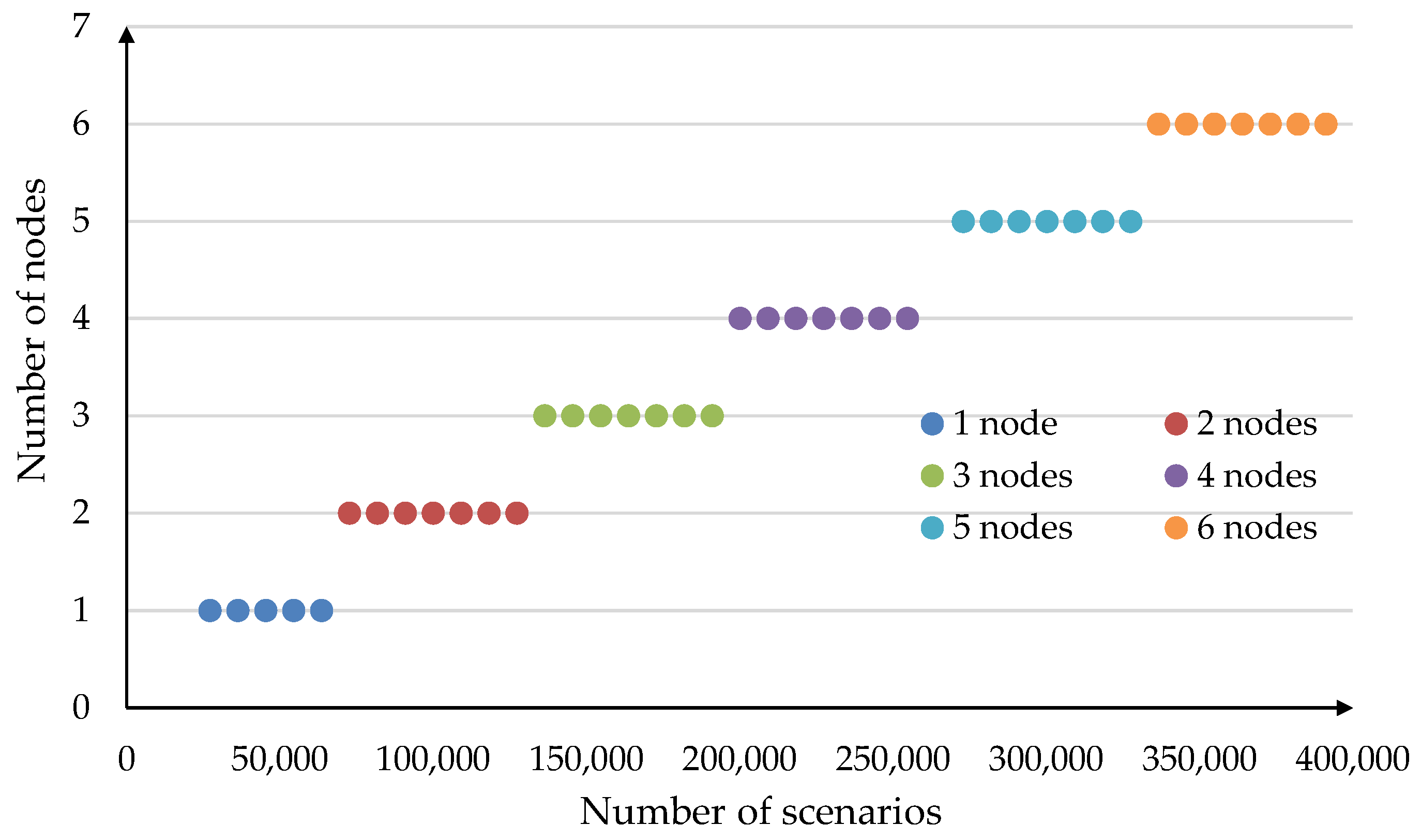
Let us demonstrate an example of the function $f_i$ evaluation. As for the ith resource, we consider the first segment of the HPC cluster at the Irkutsk Supercomputer Center [39]. The cluster node has the following characteristics: 2 × 16 cores CPU AMD Opteron 6276, 2.3 GHz, 64 GB RAM. To evaluate the minimum number of nodes required for the Apache Ignite cluster, we changed the number of scenarios from 27,300 to 391,300 in increments of 9100. 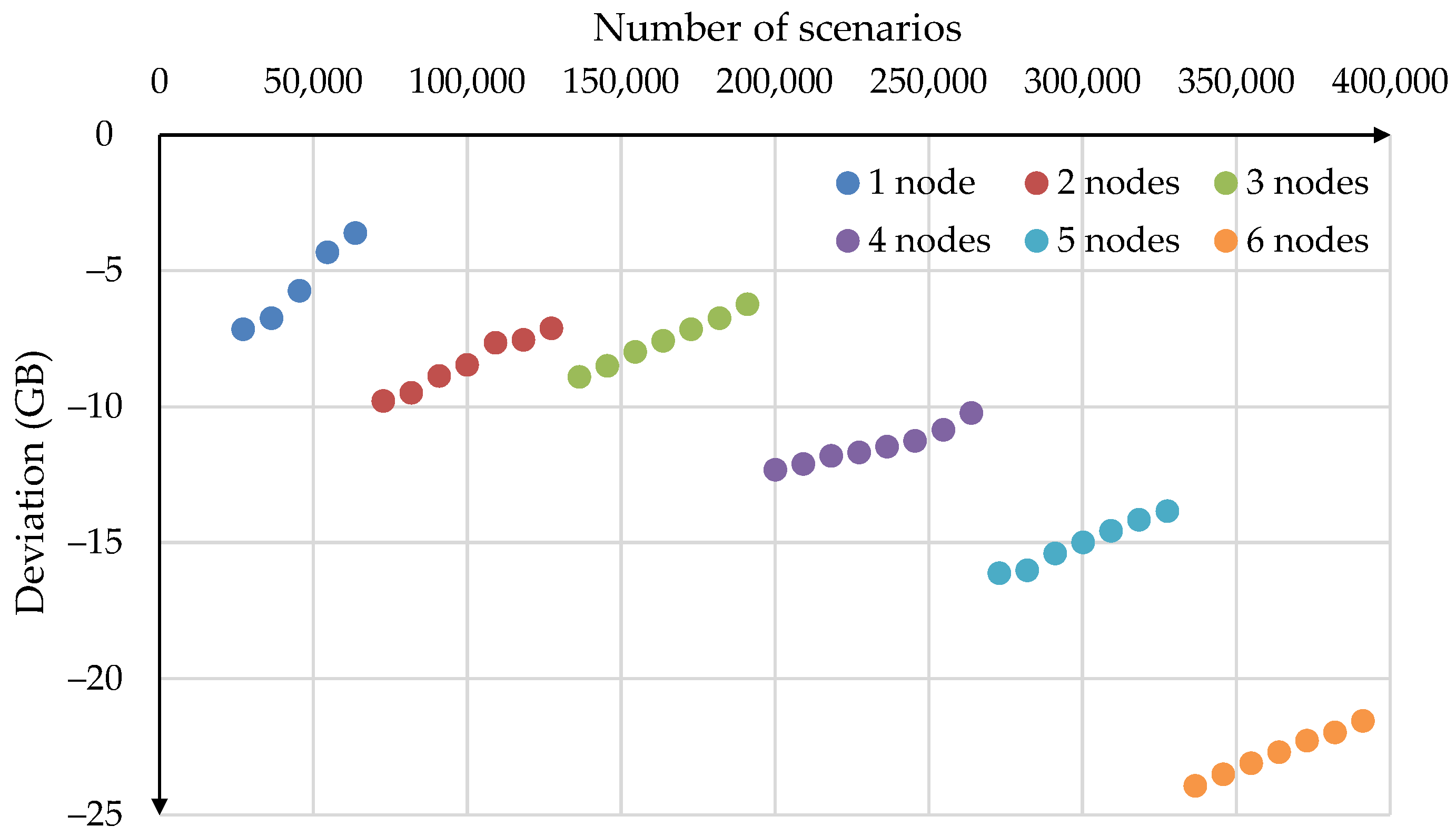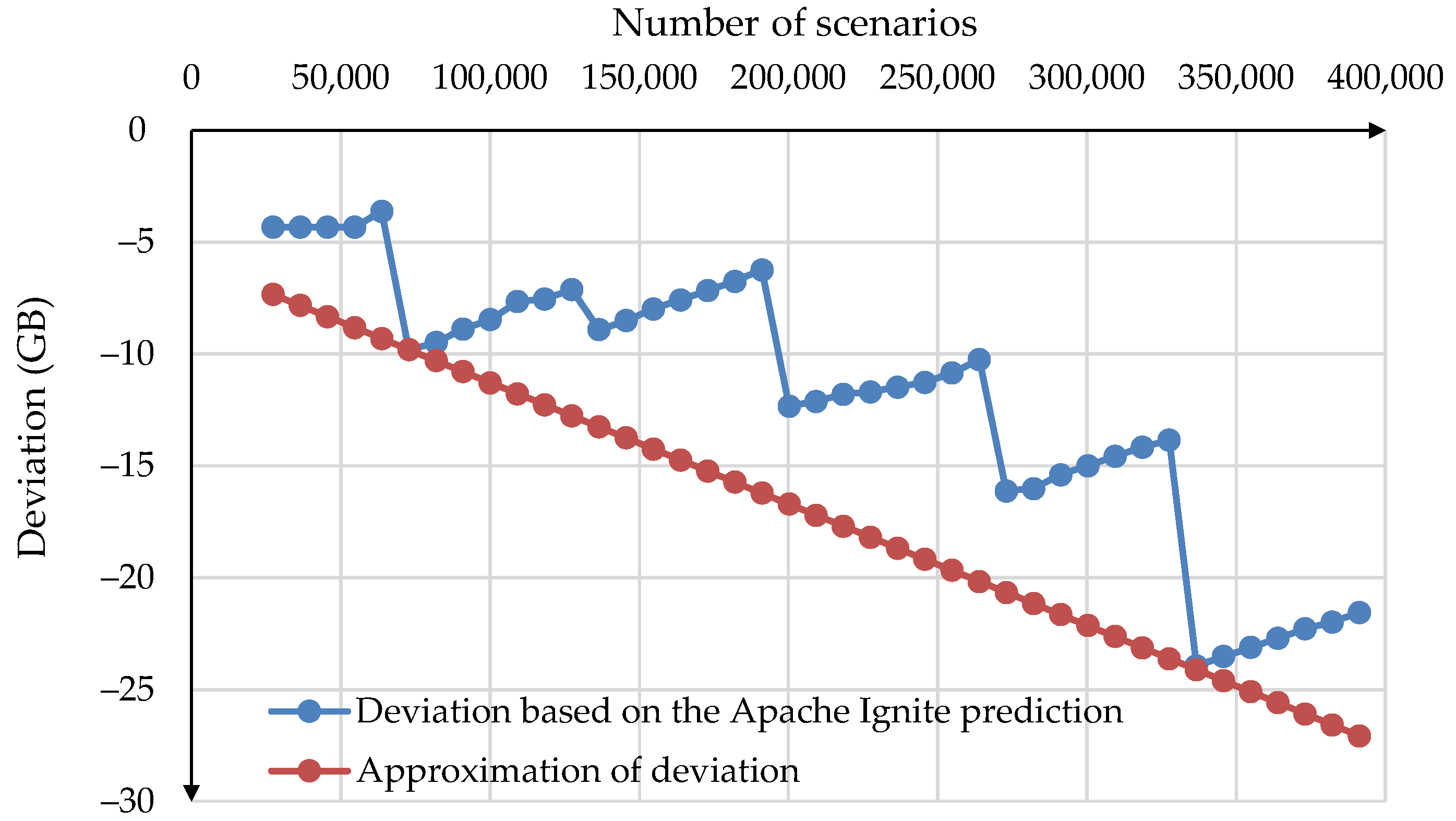Figure 2 shows the predicted number of nodes.

Figure 2. Predicted number of nodes.

Figure 3 shows the deviation of the predicted $d_i^r$ from the actual test required memory size in GB for one, two, three, four, five, and six nodes of this cluster.

Figure 3. Deviation of predicted data from test data for different numbers of nodes.

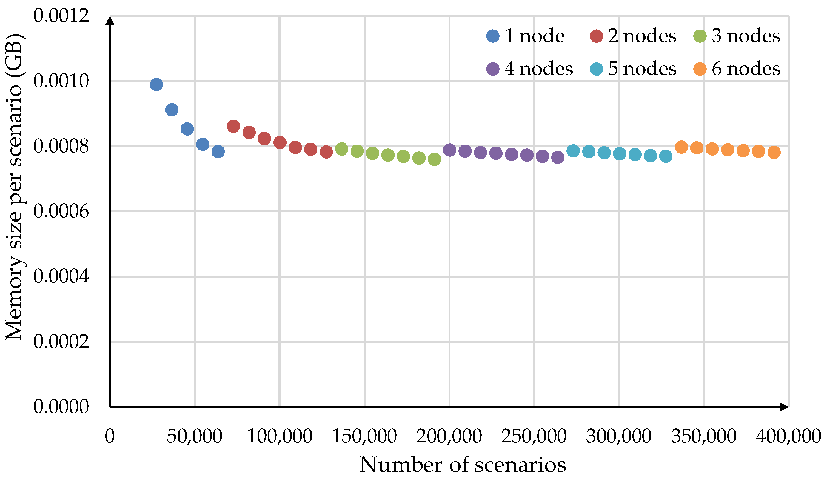
When the Apache Ignite cluster node is launched, Apache Ignite reserves a large number of memory blocks for hash tables. With a small number of disturbance scenarios, the fill density of these blocks is low. Therefore, the memory size per scenario is quite large. As the number of scenarios increases, the fill density of memory blocks grows, and the memory size per scenario decreases (Figure 4). This process is repeated after a new node is added to the Apache Ignite cluster. This explains the non-monotonic, abrupt, and intermittent nature of the deviation changes in Figure 3.

Figure 4. Changing the memory size per scenario.

We search for the linear approximation function $f_i\left(n_i^s\right)=a_i{n}_i^s+b_i$ by solving the following optimization problem using the simplex method:

$${\sum }_{\begin{array}{c}{n}_i^s=\overline{n_{i,0}^s,n_{i,k}^s}\\ with the step j\end{array}}\left(f_i^{*}\left(n_i^s\right)-f_i\left(n_i^s\right)\right)\to min,$$

(4)

$$0\le f_i^{*}\left(n_i^s\right)-f_i\left(n_i^s\right)\le 10,$$

(5)

where $f_i^{*}$ is a function of deviations shown in Figure 4, $n_{i,0}^s=\mathrm{27,300}$,$n_{i,k}^s=\mathrm{391,300}$, and $j=9100$.

Based on (4) and (5), we obtain the linear function

$$f_i\left(n_i^s\right)=-5\times {10}^{-5}{n}_i^s-5.852$$

(6)

that approximates the deviations from below (see Figure 5). In Figure 5, $d_1^e=0$.

Figure 5. Approximation of deviation.

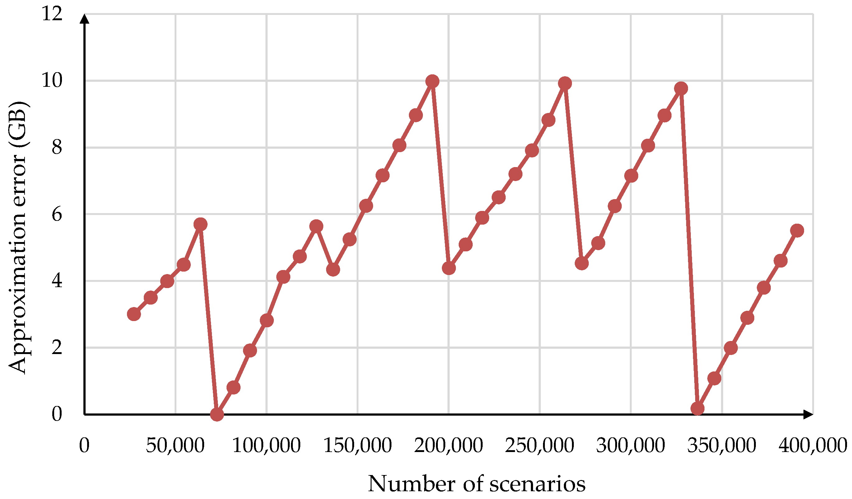
Figure 6 demonstrates the approximation error in absolute values that changed from 0 to 10 GB. Therefore, additional research is needed to reduce the observed approximation error in the future. However, applying function (6) provides the necessary evaluation of the required memory to correctly allocate the number of the Apache Ignite cluster nodes.

Figure 6. Approximation error.

3.2. Vulnerability Model

GVA is based on identifying the strongest disturbance scenarios with the most serious consequences for the energy infrastructure. $w=(w_1,w_2,\dots ,w_{n_w})$ is a vector of vulnerabilities of $n_w$ energy infrastructure configurations. Then, the problem of determining the most severe vulnerability for an energy infrastructure configuration is formulated as follows:

$$w\left(S,\left[a,b\right]\right)\to max,$$

(7)

$$g_i\left(S,Z\right)\le 0,i=1,\dots ,n_i,$$

(8)

$$h_j\left(S,Z\right)=0,j=1,\dots ,n_j,$$

(9)

$$S=⟨G,X,C⟩,$$

(10)

where

• $S$ is a set of the energy infrastructure states on which the disturbance scenarios from $Z$ are imposed;
• $a$ and $b$ are the bounds of a curve segment that reflects the rapid drop of the performance $P\left(t\right)$ on time;
• $Z$ is a generated set of disturbance scenarios;
• $g_i$ and $h_j$ are constraints of the energy infrastructure model imposed on $S$, taking into account the disturbance scenario impact from $Z$;
• $G$ and $X$ are the given structure (network) and performance limits of energy infrastructure objects;
• $C$ is environmental conditions.

The solution of the problem (7)–(10) for the configuration is the strongest disturbance scenario found by the brute-force method on $Z$.

3.3. Algorithms

Let us consider the algorithms used at the preliminary and target computing stages. Algorithms 1 and 2 represent the stage of the preliminary computing. The A1 pseudo code for modeling one series of disturbance scenarios is given below. In the Algorithm 1 description, we use the following notations:

• $G=⟨V,U⟩$ is a directed graph representing the energy infrastructure network, where $V$ is a set of vertices (possible sources, consumers of energy resources, and other objects of energy infrastructure) and $U$ is a set of edges (energy transportation ways);
• $n_e$ is a number of energy infrastructure elements from the set $E=(e_1,e_2,\dots ,e_{n_e})$, selected for random failure simulation;
• $k$ is a number of randomly failed elements;
• $Z_k$ is a set of generated disturbances (a set of combinations of $n_e$ by $k$ element failures from $E$);
• $z_k^i:w\to max$ is the strongest disturbance scenario from $Z_k$ for the ith series;
• $w_k^i$ is a set of the most negative changes in the vulnerability corresponding $z_k$ for the ith series.

Algorithm 1: Modeling Disturbance Scenarios
Inputs: $G$, $n_e$, $E=(e_1,e_2,\dots ,e_{n_e})$ Outputs: $w_1^i,w_2^i,\dots ,w_{n_e}^i$
1	$\mathbf{b}\mathbf{e}\mathbf{g}\mathbf{i}\mathbf{n}$
2	$k=1;$
3	$\mathbf{w}\mathbf{h}\mathbf{i}\mathbf{l}\mathbf{e} k\le n_e \mathbf{d}\mathbf{o}$
4	$generate\left(G,E,k\to Z_k\right)$;
5	$calculate\left(G,E,k,Z_k\to z_k^i,w_k^i\right)$;
6	$k=k+1;$
7	$\mathbf{e}\mathbf{n}\mathbf{d} \mathbf{d}\mathbf{o}$
8	$\mathbf{e}\mathbf{n}\mathbf{d}$

The Algorithm 2 is briefly described below. It determines the minimum number of disturbance scenarios series required to achieve convergence of the GVA results. In the Algorithm 2 description, we use the following notations:

• $r_0\ge 1$ is the initial number of computational experiments;
• $q$ is a number of disturbance scenarios series in each rth computational experiment;
• $\epsilon \ge 0$ is the given computation accuracy;
• $l$ is the minimum required number of disturbance scenarios series to perform GVA;
• ${\tilde{p}}_k^r$ is the average performance value in the computational experiment $r$ on the kth disturbance scenario;
• $∆{\tilde{p}}_k^{r,r-1}$ is the difference between (r − 1)th and rth computational experiments on the kth disturbance scenario;
• $\overline{∆{\tilde{p}}^{r,r-1}}$ is the average (statistical mean) of the set of values $∆{\tilde{p}}_k^{r,r-1}$;
• ${\sigma }^{r,r-1}$ is the standard deviation of the set of differences $∆{\tilde{p}}_k^{r,r-1}$.

Algorithm 2: Determing the Number of Disturbance Scenarios
Inputs: $G$, $n_e$, $E=(e_1,e_2,\dots ,e_{n_e})$, $r_0$, $q$, $\epsilon$ Outputs: $l$
1	$\mathbf{b}\mathbf{e}\mathbf{g}\mathbf{i}\mathbf{n}$
2	$r=r_0$;
3	$\mathbf{f}\mathbf{o}\mathbf{r} i=\overline{1,rq} \mathbf{s}\mathbf{t}\mathbf{e}\mathbf{p} 1 \mathbf{d}\mathbf{o}$
4	$A1\left(G,n_e,E\to w_1^i,w_2^i,\dots ,w_{n_e}^i\right)$;
5	$\mathbf{e}\mathbf{n}\mathbf{d} \mathbf{d}\mathbf{o}$
6	$\mathbf{f}\mathbf{o}\mathbf{r} k=\overline{1,n_e} \mathbf{s}\mathbf{t}\mathbf{e}\mathbf{p} 1 \mathbf{d}\mathbf{o}$
7	${\tilde{p}}_k^r=\frac{1}{q}\sum _{i=1}^q{w}_k^i$;
8	$\mathbf{e}\mathbf{n}\mathbf{d} \mathbf{d}\mathbf{o}$
9	$\mathbf{i}\mathbf{f} r=r_0 \mathbf{t}\mathbf{h}\mathbf{e}\mathbf{n} r=r+1; \mathbf{g}\mathbf{o}\mathbf{t}\mathbf{o}$ 3
10	$\mathbf{f}\mathbf{o}\mathbf{r} k=\overline{1,n_e} \mathbf{s}\mathbf{t}\mathbf{e}\mathbf{p} 1 \mathbf{d}\mathbf{o}$
11	$∆{\tilde{p}}_k^{r,r-1}=\left|{\tilde{p}}_k^r-{\tilde{p}}_k^{r-1}\right|$;
12	$\mathbf{e}\mathbf{n}\mathbf{d} \mathbf{d}\mathbf{o}$
13	${\sigma }^{r,r-1}=\sqrt{\frac{\sum _{k=1}^{n_e}{\left(∆{\tilde{p}}_k^{r,r-1}-\overline{∆{\tilde{p}}^{r,r-1}}\right)}^2}{n_e}}$;
14	$\mathbf{i}\mathbf{f} {\sigma }^{r,r-1}\ge \epsilon \mathbf{t}\mathbf{h}\mathbf{e}\mathbf{n} r=r+1; \mathbf{g}\mathbf{o}\mathbf{t}\mathbf{o}$ 3;
15	$l=rq$;
16	$\mathbf{e}\mathbf{n}\mathbf{d}$

The primary purpose of the target computing stage is to plot the dependence of the average performance value ${\tilde{p}}_k$ on the $k$ failed elements of the considered energy infrastructure. The Algorithm 3 represents the target computing stage. In the Algorithm 3 description, we use the following notations:

• $\widehat{q}\gg l$ is a number of disturbance scenarios series;
• $plot$ is a plot based on ${\tilde{p}}_1,{\tilde{p}}_2,\dots ,{\tilde{p}}_{\widehat{q}}$.

Algorithm 3: Target Computing
Inputs: $G$, $n_e$, $E=(e_1,e_2,\dots ,e_{n_e})$, $\widehat{q}$ Outputs: $plot$
1	$\mathbf{b}\mathbf{e}\mathbf{g}\mathbf{i}\mathbf{n}$
2	$\mathbf{f}\mathbf{o}\mathbf{r} i=\overline{1,\widehat{q}} \mathbf{s}\mathbf{t}\mathbf{e}\mathbf{p} 1 \mathbf{d}\mathbf{o}$
3	$A1\left(G,n_e,E\to w_1^i,w_2^i,\dots ,w_{n_e}^i\right)$;
4	$\mathbf{e}\mathbf{n}\mathbf{d} \mathbf{d}\mathbf{o}$
5	$\mathbf{f}\mathbf{o}\mathbf{r} k=\overline{1,n_e} \mathbf{s}\mathbf{t}\mathbf{e}\mathbf{p} 1 \mathbf{d}\mathbf{o}$
6	${\tilde{p}}_k=\frac{1}{\widehat{q}}\sum _{i=1}^{\widehat{q}}{w}_k^i$;
7	$\mathbf{e}\mathbf{n}\mathbf{d} \mathbf{d}\mathbf{o}$
8	$plotting\left({\tilde{p}}_1,{\tilde{p}}_2,\dots ,{\tilde{p}}_{n_e}\to plot\right)$;
9	$\mathbf{e}\mathbf{n}\mathbf{d}$

4. Application

We use the OT framework to develop and apply a scientific application for studying the resilience of energy infrastructures. The first version of this application includes workflows for studying vulnerability as a key metric of resilience.

OT includes the following main components:

• User interface;
• Designer of a computational model that implements the knowledge specification about the subject domain of solved problems;
• Converter of subject domain descriptions (an auxiliary component of the computational model designer), represented in domain-specific languages, into the computational model;
• Designer of module libraries (auxiliary component of the computational model designer) that support the development and modification of applied and system software;
• Software manager that provides continuous integration of applied and system software;
• Computation manager that implements computation planning and resource allocation in a heterogeneous distributed computing environment;
• Computing environment state manager that observes resources;
• API for access to external information, computing systems, and resources, including digital platform of ecological monitoring of BNT [40];
• Knowledge base about computational model and computation databases with the testing data, initial data, and computing results.

The conceptual model contains information about the scientific application, which has a modular structure. The model specifies sets of parameters, abstract operations on the parameter field, applied and system software modules that implement abstract operations, workflows, and relations between the listed objects. In addition, this model describes the hardware and software infrastructure (characteristics of nodes, communication channels, network devices, network topology, etc.). OT provides the development of system modules that implement computing environment monitoring, interacting with meta-schedulers, local resource managers, and IMDG middleware, transferring, pre- and post-processing of data, etc. System operations and modules can be included in the computational model and executed within workflows.

End-users of the application execute workflows to perform computational experiments. The computation manager controls the workflow executions in the computing environment. It receives information about the state of computing processes and resources from the manager of the computing environment state. In addition, the computation manager can visualize the calculated parameters and publish workflows as WPSs on the digital platform of ecological monitoring using the API mentioned above.

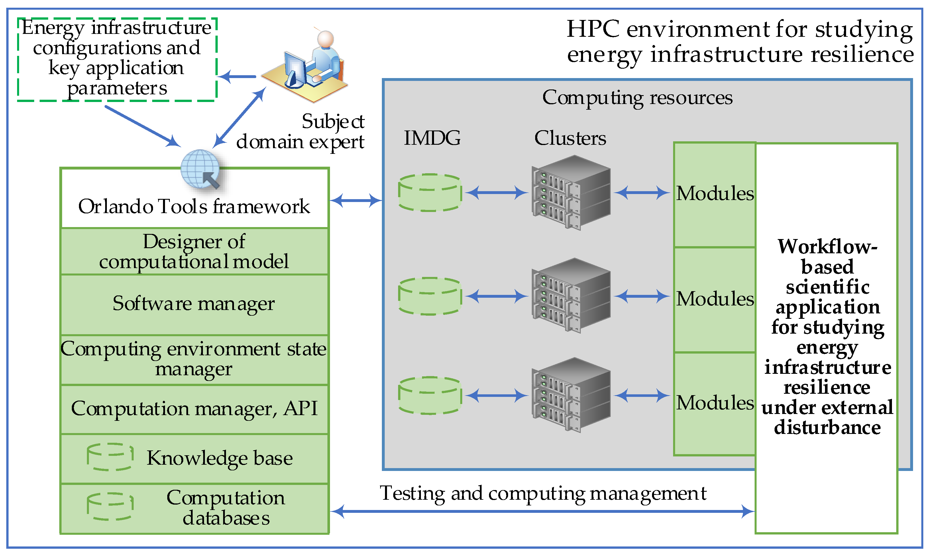
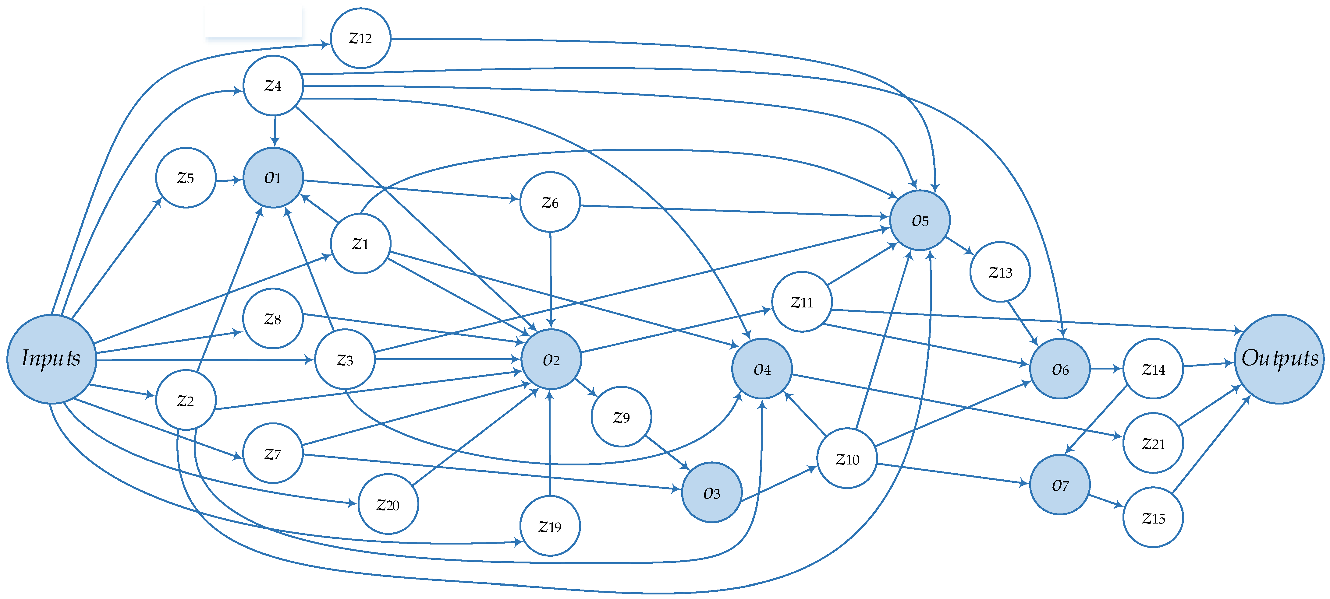
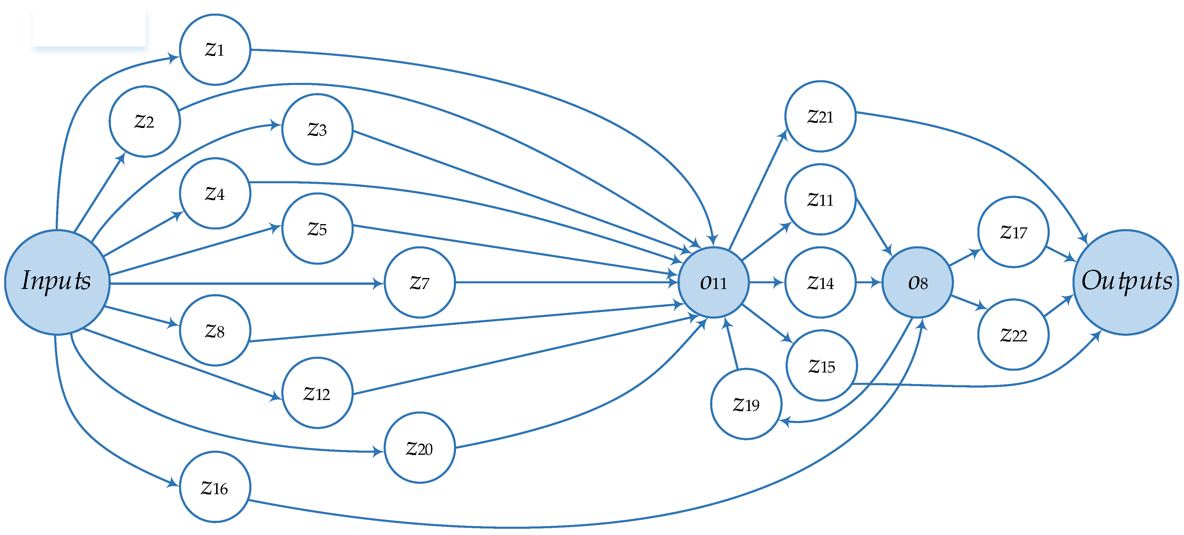
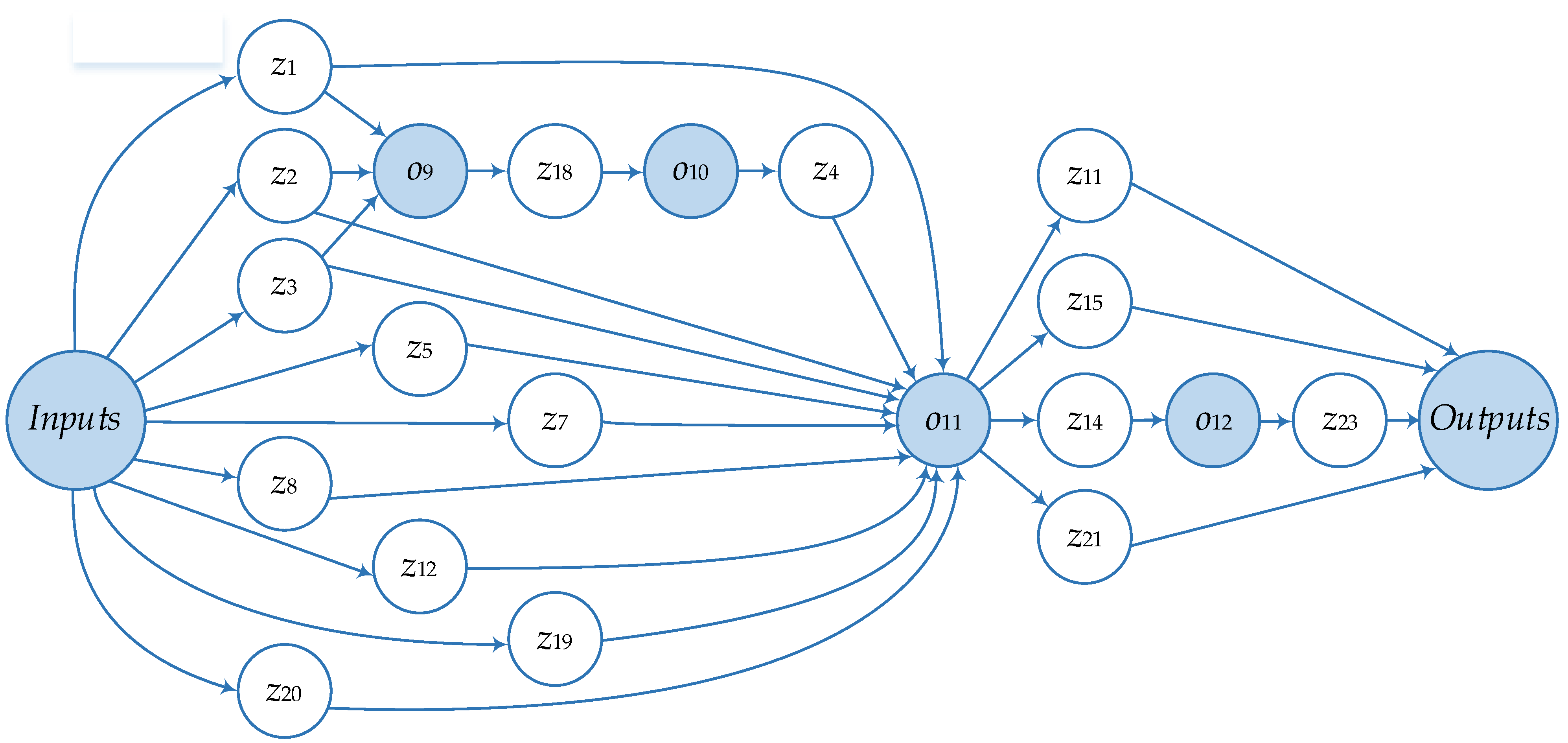
Figure 7 shows the structure of the HPC environment. The debugged and tested applied software within the testing stage is deployed on resources (computational clusters) of the environment. At the preliminary and target stages, the subject domain expert interacts with the OT components, sets initial data (energy infrastructure configurations and key application parameters), executes application workflows, controls their completion, and obtains and evaluates computation results. Workflows for GVA are shown in Figure 8, Figure 9 and Figure 10. The inputs and outputs elements represent the input and output data of workflows, respectively.

Figure 7. HPC environment structure.

Figure 8. Workflow 1.

Figure 9. Workflow 2.

Figure 10. Workflow 3.

Workflow 1 computes the decrease in the energy system performance with the given configuration due to mass failures of its elements. Operation $o_1$ retrieves a list of energy system elements from the computation database. Then, operation $o_2$ determines the required number of nodes to form an Apache Ignite IMDG cluster and configures its nodes. Next, operation $o_3$ launches an instance of the IMDG cluster, to which operation $o_4$ writes the structure of the energy system. Operation $o_5$ models a series of disturbances. The results of its execution are aggregated by the operation $o_6$. IMDG cluster nodes are stopped and released by the operation $o_7$.

Workflow 2 implements an algorithm for searching the minimum number of disturbance scenarios series required to obtain a stable evaluation of the decrease in the energy system performance. It is executed within the preliminary computing stage and applied to one energy infrastructure configuration selected by the subject domain specialist. Operation $o_{11}$ reflects Workflow 1. Operation $o_8$ checks whether the required minimum number of disturbance scenarios has been achieved. If the condition $\left(z_{11}\ne z_{20}\right)\wedge \left(z_{17}<z_{16}\right)$ is true, then Workflow 2 is completed. Otherwise, $r$ is incremented by one and a new experiment is performed.

Workflow 3 realizes the target computing stage. Operation $o_9$ extracts a set of configurations of the energy system under study from the computation database. Operation $o_{10}$ decomposes the general problem into separate subproblems, where one configuration is processed in parallel by an instance of operation $o_{11}$. The input parameter $z_{20}$ has the initial value equal $\widehat{q}$. Finally, operation $o_{12}$ draws the plot.

The parameters $z_1-z_{22}$ are inputs and outputs of operations, where:

• $z_1$, $z_2$, and $z_3$ determine the graph $G$;
• $z_4$ is an energy infrastructure configuration ID;
• $z_5$ is a type of energy infrastructure elements;
• $z_6$ represents the set $E$ and the number $n_e$ of its elements;
• $z_7$ is a set of options for the Apache Ignite cluster;
• $z_8$ is a list of $d_i^n$, $i=\overline{1,n_r}$;
• $z_9$ is a list of $n_i$, $i=\overline{1,n_r}$;
• $z_{10}$ is a list of node network addresses of the Apache Ignite cluster;
• $z_{11}$ and $z_{12}$ represent $r$ and $q$, correspondingly;
• $z_{13}$ is a list of $w_k^i$, $i=\overline{1,rq}$, $k=\overline{1,n_e}$;
• $z_{14}$ is a list of ${\tilde{p}}_k^r$ for rth computational experiment, $k=\overline{1,n_e}$;
• $z_{15}$ is the exit code of the operation $o_7$;
• $z_{16}$ and $z_{17}$ specify $\epsilon$ and $s$, correspondingly;
• $z_{18}$ is a list of energy infrastructure configuration IDs;
• $z_{19}$ and $z_{20}$ determine $r+1$ and $r_0$, correspondingly;
• $z_{21}$ is a log file;
• $z_{22}$ represents $l$;
• $z_{23}$ is a plot.

To distribute a set of scenarios among the resources that are available to run the experiment, the OT computation manager solves the following optimization problem:

$$\tau =\underset{i=\overline{1,n_r}}{\max }\left({\mu }_i\right)\to min,$$

(11)

$${\mu }_i={ϵ}_i+\frac{{\nu }_i}{{\eta }_i{\pi }_i},$$

(12)

$${\sum }_{i=1}^{n_r}{\nu }_i=n_s, 0\le {\mu }_i\le {\delta }_i, {\eta }_i^{min}\le {\eta }_i\le {\lambda }_i,$$

(13)

where

• ${ϵ}_i$ is overheads for the use of the ith resource independent of the number of scenarios;
• ${\nu }_i$ is a number of scenarios under processing on the ith resource;
• ${\eta }_i$ is the number of nodes dedicated to the ith resource;
• ${\pi }_i$ is a performance of the ith resource defined by the ratio of the number of scenarios per unit of time;
• ${\delta }_i$ is a quota on time-of-use of the ith resource for problem solving;
• ${\lambda }_i$ is a quota on a number of nodes of the ith resource for problem solving;
• ${\eta }_i^{min}\ge 1$ is the minimum number of nodes of the ith resource considering the required memory size for IMDG.

In this problem Formulation (11)–(13), minimization ensures a rational use of resources and balancing of their computational load. The resources used may have different computational characteristics of their nodes. Redistribution for part of the computing load from faster to slower nodes can be encouraged if the makespan of the workflow execution is reduced.

5. Computational Experiments

We performed GVA for an energy infrastructure model similar to one of the segments for the gas transportation network in Europe and Russia. This model includes 910 elements, including 332 nodes (28 sources, 64 consumers, 24 underground storage facilities, and 216 compressor stations) and 578 sections of main pipelines and branches of distribution networks. The total amount of natural gas supplied to consumers was chosen as the performance measure $P\left(t\right)$ for this segment of the gas supply network. The measure $P\left(t\right)$ is normalized by converting the resulting supply value into a percentage of the required total energy demand following [4].

Computational experiments were performed in the heterogeneous distributed computing environment on the following resources:

• HPC Cluster 1 with the following node characteristics: 2 × 16 cores CPU AMD Opteron 6276, 2.3 GHz, 64 GB RAM;
• HPC Cluster 2 with the following node characteristics: 2 × 18 cores CPU Intel Xeon X5670, 2.1 GHz, 128 GB RAM;
• HPC Cluster 3 with the following node characteristics: 2 × 64 cores CPU Kunpeng-920, 2.6 GHz, 1 TB RAM.

The HPC clusters used for the experiments are geographically distributed and have different administrative affiliations. Therefore, we consider our experimental computing environment consisting of resources from these clusters as a computational grid [41].

Below are the results of the preliminary and target computing.

The search for the minimum number of series of disturbance scenarios is performed by increasing the initial value of the number of sequences. We increase the number of sequences until the convergence of the results of two GVA iterations, determined by the value of $\epsilon$, is achieved. Due to the high degree of uncertainty in the data characterizing the behavior of the selected gas supply network under conditions of major disturbances, we use $\epsilon$ equal to 0.025%.

We started the preliminary computing with $r_0=1$ and $q=5$. The minimum required number of disturbance scenario series was found at $r=200$. Therefore, $l=1000$. Next, according to the GVA methodology [6], we set $\widehat{q}$ equal to 2000 and $r$ equal to 400 to perform the target computing.

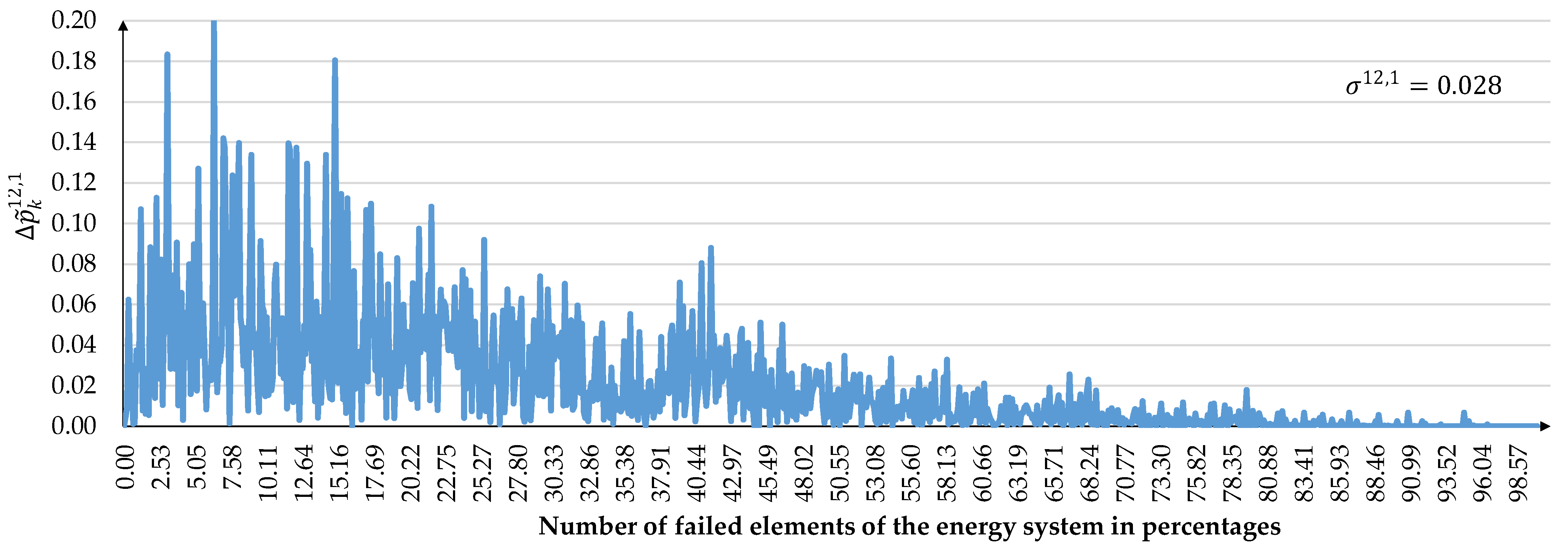
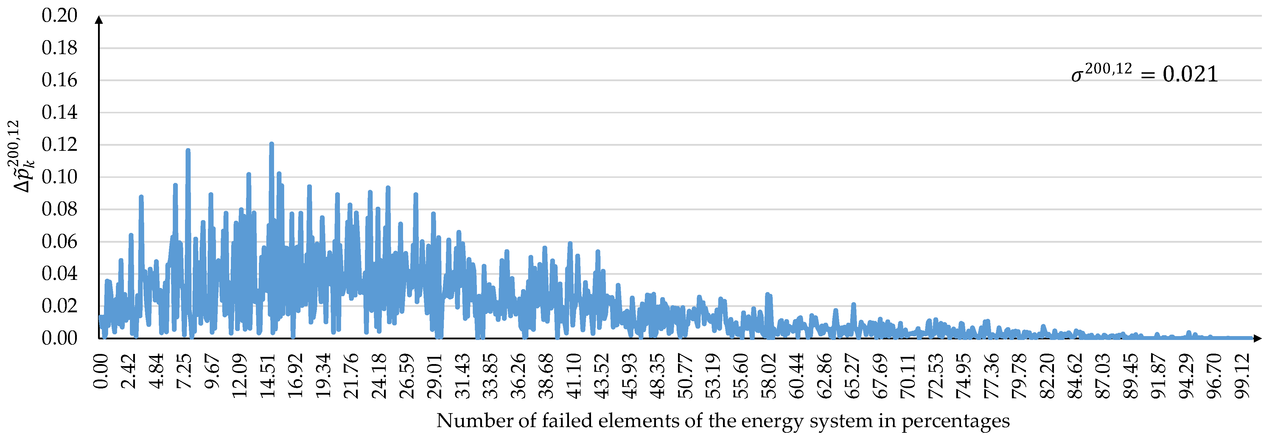
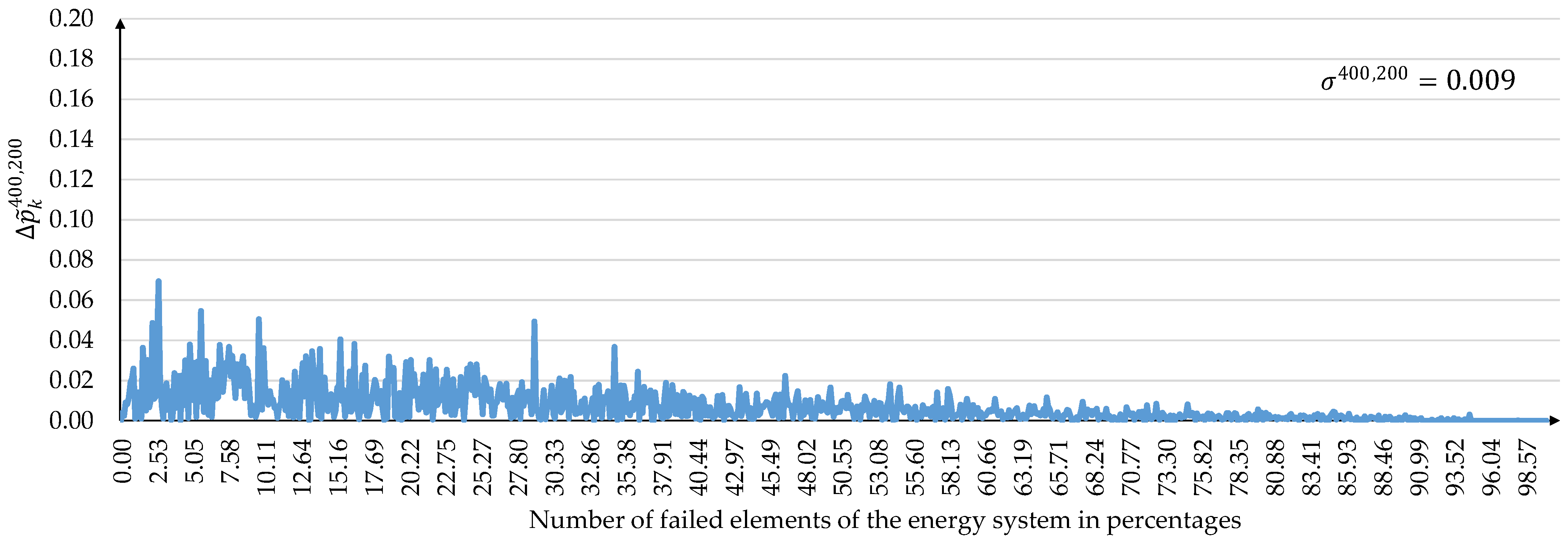
The convergence process for the experimental results is illustrated in Figure 11, Figure 12 and Figure 13. These figures show the graphs of $∆{\tilde{p}}_k^{\mathrm{12,1}}$, $∆{\tilde{p}}_k^{\mathrm{200,12}}$, and $∆{\tilde{p}}_k^{\mathrm{400,200}}$, which reflect the difference in performance degradation between the following pairs of computational experiments: ($r=1, r=12$), ($r=12, r=200$), and ($r=200, r=400$). The difference in the consequences of large disturbances is given on the y-axis. The x-axis represents the amplitude of large disturbances, expressed as a percentage of the number of failed elements. In addition, the standard deviations ${\sigma }^{\mathrm{12,1}}=0.028$, ${\sigma }^{\mathrm{200,12}}=0.021$, and ${\sigma }^{\mathrm{400,200}}=0.009$ are shown in the upper right corners of the corresponding figures.

Figure 11. Graph of $∆{\tilde{p}}_k^{\mathrm{12,1}}$.

Figure 12. Graph of $∆{\tilde{p}}_k^{\mathrm{200,12}}$.

Figure 13. Graph of $∆{\tilde{p}}_k^{\mathrm{400,200}}$.

Figure 11, Figure 12 and Figure 13 show that the largest scatters in the difference between the consequences of large disturbances occur at the initial values of $k$. They then decrease as $k$ increases. The magnitude of the dispersion is determined by the criticality of the network elements, whose failures are modeled in disturbance scenarios. This is especially noticeable for small values of $k$. The consequences of failures of some critical elements for a selected segment of the natural gas transportation network can reach 10% or more. At the same time, failures of most non-critical elements do not significantly affect the supply of natural gas to consumers. As $k$ increases, the dependence on the criticality of failed network elements decreases. This leads to a decrease in the spread of the difference in the consequences of large disturbances. In general, the above results of target computing are consistent with the results in [6].

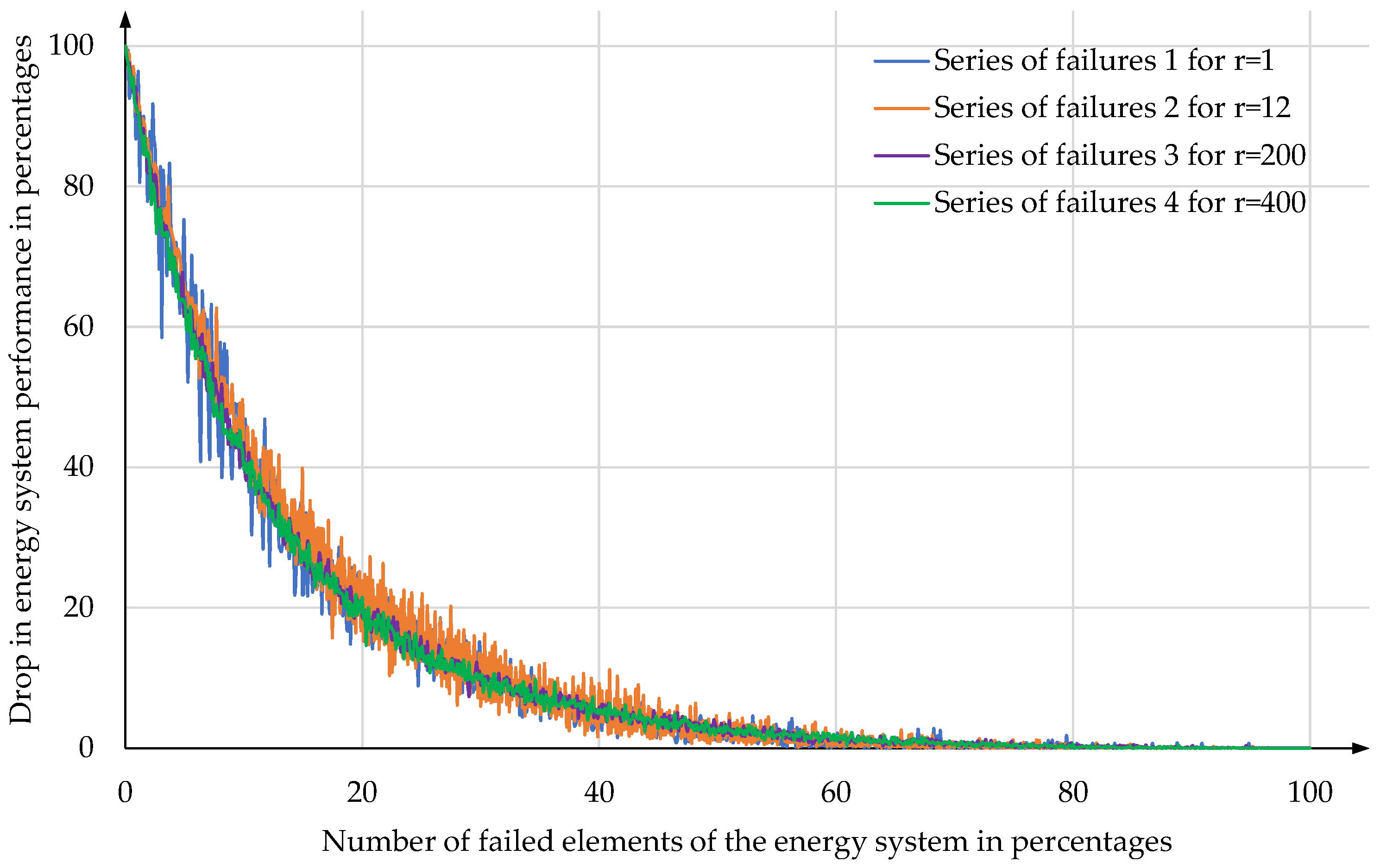
Figure 14 shows the drop in the performance for the energy system segment under consideration. The drop is shown depending on the number of its failed elements for various failures. We can see that serious problems in gas supply to consumers begin already with a small number of failed elements, which is about 3%. Here, a serious problem in gas supply means a drop in the performance by 20% or more.

Figure 14. Decreasing the energy system performance.

Table 3 provides several important quantitative characteristics of GVA for various technical systems [42,43,44,45,46,47,48], including the considered segment of the gas supply system. A more detailed comparison in dependences of system vulnerabilities on disturbance amplitudes is difficult to perform even at a qualitative level. This is due to the following reasons.

Table 3. Characteristics of experiments.

System	Literary Source	Resource	Number of Vertices	Number of Edges	Maximum Number of Simultaneously Failed Elements	Failed Elements
A small town power system	[42]	Power	352	452	804	All vertices and edges
Net3	[43]	Water	97	119	119	All edges
OBCL-1	[43]	Water	263	289	289	All edges
D-town	[43]	Water	407	459	459	All edges
Ky14	[43]	Water	384	553	553	All edges
Ky3	[43]	Water	275	371	371	All edges
80 virtual networks	[43]	Water	102–506	110–554	554	All edges
Our infrastructure	-	Natural gas	332	578	910	All vertices and edges
Soviet rail system circa 1955	[44]	Railway	50	89	7	Edges
Provincial pipeline network	[45]	Natural gas	35	34	10	Edges
A transmission network	[46]	Natural gas	54	70	70	All edges
IEEE 118 bus system	[47]	Power	118	186	10	Edges
IEEE 118 bus system	[48]	Power	118	186	30	Vertices and edges
IEEE 30 bus system	[48]	Power	30	41	10	Vertices and edges

• There are differences in the types of systems under study and the details of representing the distribution of resource flows across systems in their models. For example, for simple linear models of railway transport [44], gas supply [45,46], and electricity supply [42,47,48], it is sufficient to use only information about the capacity of system network edges. At the same time, the nonlinear water supply model requires additional considerations of the pressure in nodes (network vertices) and the hydraulic resistance of edges. In [48], in contrast to [42,47], the additional possibility of a cascading propagation of accidents throughout the system during the impact of a major disturbance is taken into account. In our study, we use a gas supply model similar to [45,46].
• The network structure of a specific system configuration largely determines its vulnerability. Xie et al. [48] clearly showed that the vulnerability dependencies on the amplitude of disturbances are significantly different for two different electrical power systems.
• Various principles of a random selection of elements for GVA are used. In our work as well as in [42], all network elements (vertices and edges) can be selected for failure (see Table 3). At the same time, in [43,44,46,47], only edges are selected. In [45,47], only edges with low centrality values are selected for failure.

Overall, our approach to GVA [49] integrates and develops the advantages of the approaches presented in [6,42]. In particular, we combine models of different energy systems to study their joint operation under extreme conditions. Such a combination is based on the unified principles of interaction with models of energy infrastructures at different levels of the territorial-sectoral hierarchy.

Our methodological result is that we have ensured that all elements (vertices and edges) of the gas transportation network can be included in the set of failed elements. This allowed us to perform a complete analysis of the production and transportation subsystems of the gas supply system in contrast to [45,46], where only edge failures were modeled. The possible synergistic effect of simultaneous failures of several network elements is important. It lies in the fact that the consequences of a group failure can be higher than the sum of the consequences of individual failures. The synergetic effect affects the curves presented in Figure 14, increasing their slope. As the search for critical elements showed in [26], the synergetic effect appears only when considering joint failures at the vertices and edges of the energy network. The steepness of the curves in Figure 14, which is greater than that of similar curves in [39], is due precisely to the synergetic effect. The system vulnerability analysis performed in [44,45,46,47] also does not consider the synergistic effect of simultaneous failures at the vertices and edges of the energy network.

Moreover, the size of the studied segment of the gas supply system significantly exceeds similar characteristics of the experiments represented in [43,44,45,46,47,48]. The network size determines the maximum number of simultaneous random failures, which is necessary to construct the dependencies in Figure 14. Xie et al. showed that 10 random attacks in [47] are not enough to conclude about the stability of an electric power system of similar size to the IEEE 118 bus system. In our experiment, the maximum number of simultaneously failed elements is equal to the number of network elements. This allows us to draw conclusions about the boundary beyond which the system collapses, i.e., breaks down into independent parts. A model with a high quality and quantity of input data delivers more founded outputs.

In Table 4, we show the experimental results for HPC Cluster 1 ($i=1$), HPC Cluster 2 ($i=2$), and HPC Cluster 3 ($i=3$). In GVA problem solving, we have processed 1,820,000 disturbance scenarios. The values of ${\eta }_i$, ${\nu }_i$, and ${\mu }_i$ are calculated based on solving the problem (11)–(13) taking into account ${\delta }_i$, ${\lambda }_i$, and ${ϵ}_i$. ${\mu }_i$ reflects the predicted data processing time (DPT) on ${\eta }_i$ nodes of the ith HPC cluster. The parameter ${\eta }_i^{min}$ is determined using (1)–(3). It sets the minimum number of nodes required for the ith Apache Ignite cluster to provide computation reliability, ${\eta }_i^{min}\le {\eta }_i$. We add ${\eta }_i-{\eta }_i^{min}$ nodes on the ith HPC cluster, $i=\overline{1,n_r}$. This balances the computing load in proportion to the node performance and decreases the real DPT on ${\eta }_i$ nodes in comparison with the predicted DPT on ${\eta }_i^{min}$ nodes. The addition of the nodes is made within the existing quotas ${\lambda }_i$. The error of ${\mu }_i$ (the DPT prediction error) does not exceed 8.15% compared to the DPT obtained in computational experiments on ${\eta }_i$ nodes.

Table 4. Data processing time and computation speedup.

i	${\mathit{\delta }}_{\mathit{i}}$ (s)	${\mathit{ϵ}}_{\mathit{i}}$ (s)	${\mathit{\lambda }}_{\mathit{i}}$	${\mathit{\eta }}_{\mathit{i}}$	${\mathit{\nu }}_{\mathit{i}}$	${\mathit{\mu }}_{\mathit{i}}$	${\mathit{\eta }}_{\mathit{i}}^{\mathit{m}\mathit{i}\mathit{n}}$	$\mathbf{DPT} \mathbf{on}$ ${\mathit{\eta }}_{\mathit{i}}^{\mathit{m}\mathit{i}\mathit{n}}$ Nodes (s)	$\mathbf{DPT} \mathbf{on}$ ${\mathit{\eta }}_{\mathit{i}}$ Nodes (s)	Error	Computation Speedup
1	1,728,000.00	120	15	15	216,230	736.61	6	1561.53	711.61	3.39	2.24
2	864,000.00	100	20	20	1,312,587	736.63	15	895.51	694.83	5.67	1.29
3	1,296,000.00	90	3	3	291,183	736.63	1	1909.89	676.63	8.15	2.82

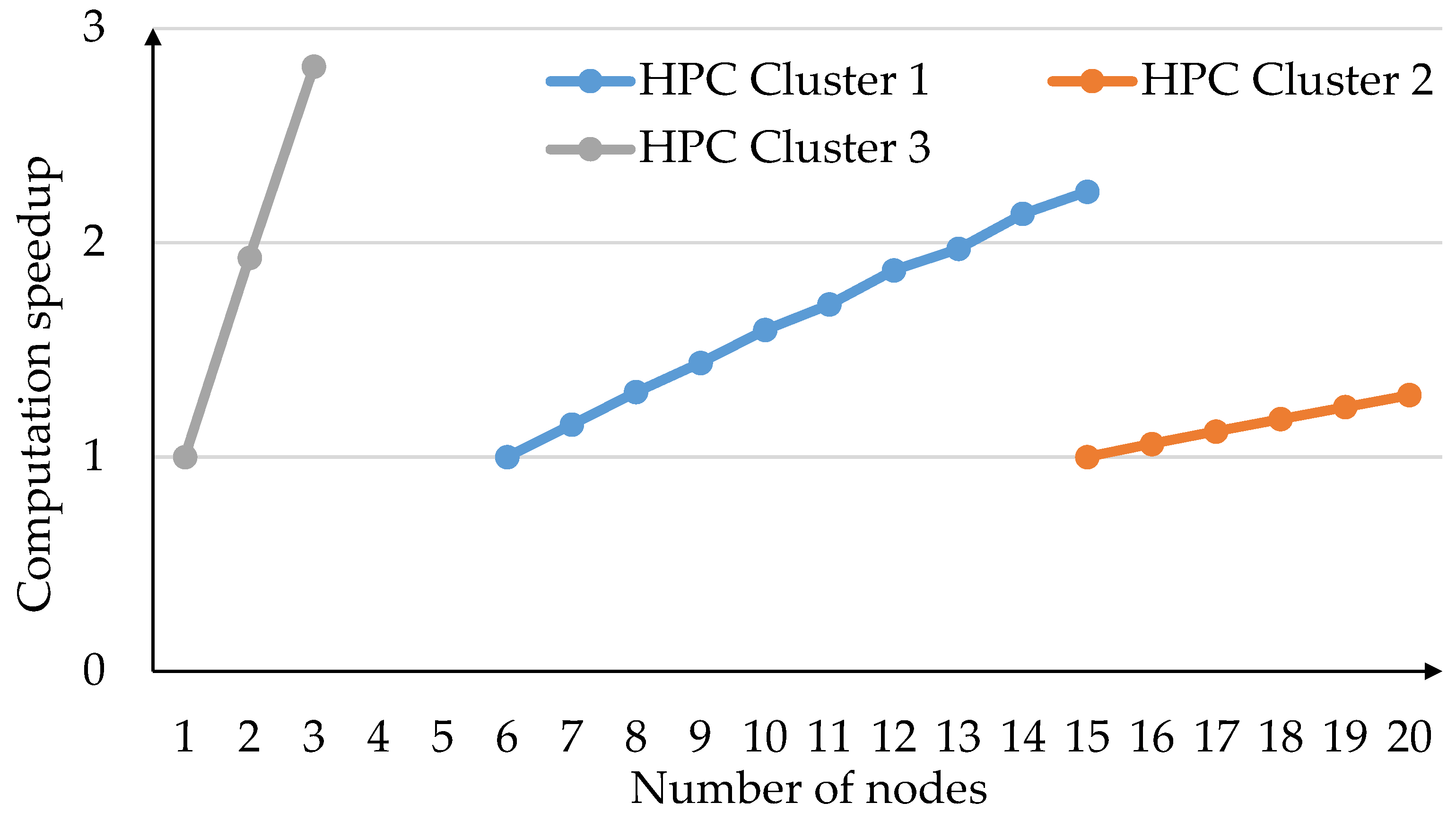
Figure 15 shows the computation speedup achieved by adding new Apache Ignite nodes on the HPC clusters. The speedup increases with the following increases in the number of nodes:

• From 6 to 15 nodes for HPC Cluster 1;
• From 15 to 20 nodes for HPC Cluster 2;
• From 1 to 3 nodes for HPC Cluster 3.

We see that the makespan $T$ is reduced by more than two times (from 1909.89 to 711.61) compared to the makespan obtained with the number of nodes required by Apache Ignite for a given problem where

$$T=\left\{\begin{array}{cc}\underset{i=\overline{1,n_r}}{\max }{\eta }_i^{min}& for DPT on {\eta }_i^{min} nodes,\\ \underset{i=\overline{1,n_r}}{\max }{\eta }_i& for DPT on {\eta }_i nodes.\end{array}\right.$$

In all three cases, the speedup is close to linear.

Figure 15. Computation speedup for the HPS clusters.

Figure 15. Computation speedup for the HPS clusters.

6. Discussion

Nowadays, studying the development and use of energy systems in terms of environmental monitoring and conservation is undoubtedly a challenge. Resilience of energy systems is one of the applications within such a study. In terms of maintaining a friendly environmental situation, conserving natural resources, and ensuring balanced energy consumption, increasing the resilience of energy systems can prevent the negative consequences of significant external disturbances.

Top-down, bottom-up, and hybrid approaches to energy modeling can be implemented at macro and micro levels with low, medium, and high data requirements. In addition, energy system models can include one sector, such as the electricity sector, or multiple sectors and assume optimization, agent-based, stochastic, indicator-based, or hybrid modeling. In all cases, large-scale experiments are considered to be repeated.

Preparing large-scale experiments for this study is quite a long and rigorous work. Within such a work, it is necessary to consider as much as possible the subject domain specificity and the end-user requirements concerning the computing environment used.

This requires the development and application of specialized tools to support different aspects of studying the resilience of energy systems. These aspects include large data sets, need to speed up their processing, demand for HPC use, convergence of applied and system software, provision of flexible and convenient service-oriented end-user access to the developed models and algorithms, etc. Therefore, it is evident that system models, algorithms, and software are required to the same extent as applied developments to provide efficient problem solving and rational resource utilization within large-scale experiments.

Unfortunately, there are no ready-made solutions in the field of resilience research for its different metrics. To this end, we focus on designing a new approach to integrate workflow-based applications with IMDG technology and WPSs to implement the resilience study for energy systems in the HPC environment.

7. Conclusions

We studied a model of a gas transportation network, represented in the form of a directed graph, taking into account external disturbances. Unlike known approaches to solving a similar problem, our approach allows the simulation of changes in the energy infrastructure performance by generating simultaneous failures of network elements (vertices and arcs of the graph) up to the failure of all infrastructure objects. The solution is characterized by high computational complexity. Therefore, we have developed a workflow-based application for modeling the vulnerability of energy infrastructure, oriented to execution on a cluster grid. The efficient data processing is implemented based on the IMDG technology. In contrast to known approaches to organizing such data processing, we automatically select, deploy, configure, and launch IMDG cluster nodes for executing workflows.

We achieve near-linear speedup in each resource due to the parallel processing of disturbance scenarios and rational distribution of the computational load for processing a series of scenarios on the different resources. We also show that the problem-solving makespan is reduced more than twice.

In addition, we develop and provide:

• WPS-oriented access to problem solving in the geosciences;
• Automatic transformation of subject domain descriptions, expressed in domain-specific languages, into a specialized computational model;
• System parameters and operations support the workflows to interact with both the computing environment and the IMDG middleware;
• Reliable computation based on testing the applied software and allocation of available nodes.

Future work will focus on the following research directions: expanding the library of scientific applications by creating new workflows to study other resiliency metrics; optimizing the prediction of the required memory for data processing on an Apache Ignite cluster; conducting large-scale experiments to study resilience concerning a complete set of metrics on existing infrastructures of fuel and energy complexes and their components using additional cloud resources.