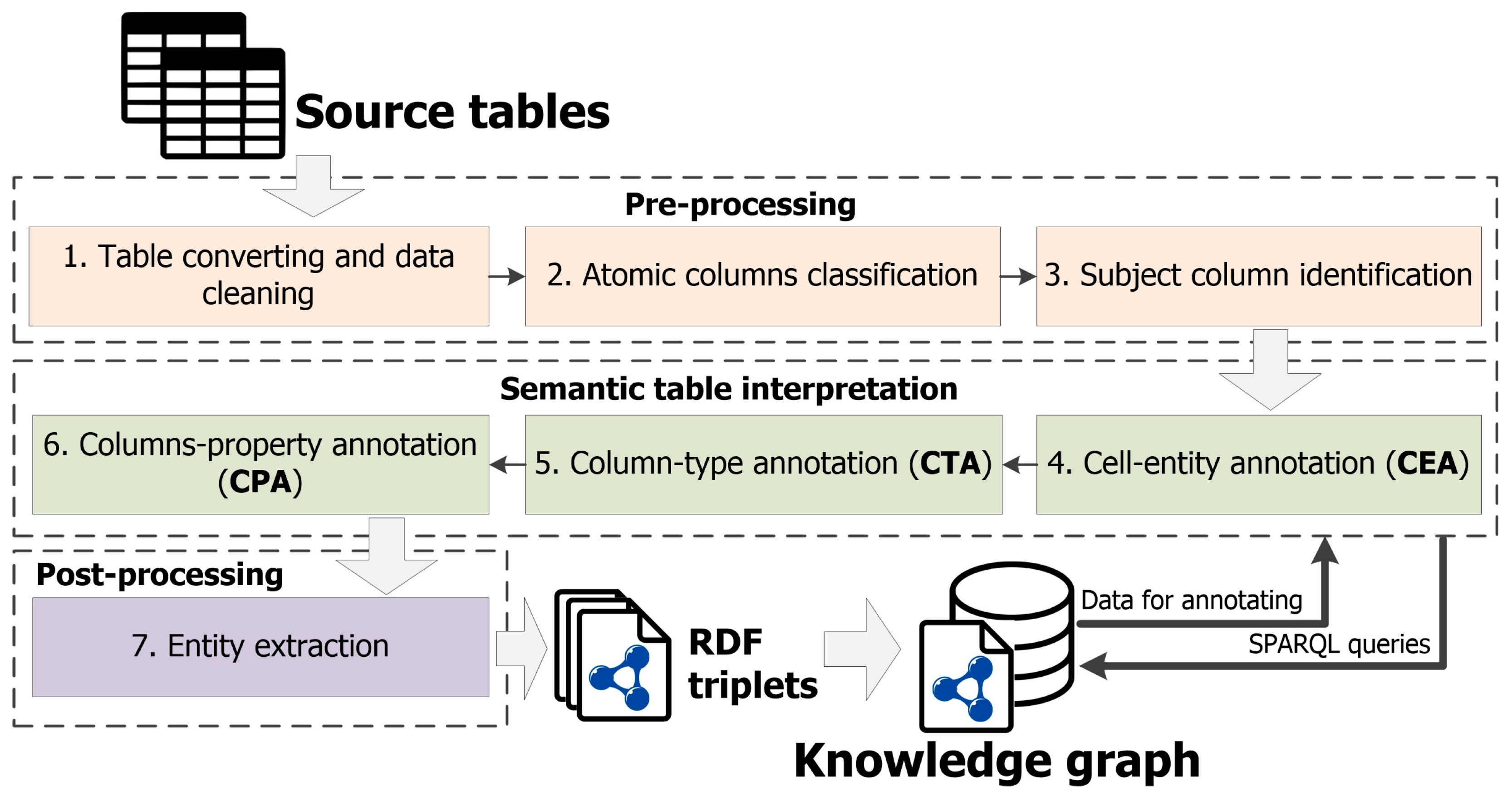
Article

Knowledge Graph Engineering Based on Semantic Annotation of Tables

Matrosov Institute for System Dynamics and Control Theory, Siberian Branch of Russian Academy of Sciences (ISDCT SB RAS), Irkutsk 664033, Russia
*
Author to whom correspondence should be addressed.
Computation 2023, 11(9), 175; https://doi.org/10.3390/computation11090175
Submission received: 10 July 2023 / Revised: 25 August 2023 / Accepted: 30 August 2023 / Published: 5 September 2023

Abstract

:
A table is a convenient way to store, structure, and present data. Tables are an attractive knowledge source in various applications, including knowledge graph engineering. However, a lack of understanding of the semantic structure and meaning of their content may reduce the effectiveness of this process. Hence, the restoration of tabular semantics and the development of knowledge graphs based on semantically annotated tabular data are highly relevant tasks that have attracted a lot of attention in recent years. We propose a hybrid approach using heuristics and machine learning methods for the semantic annotation of relational tabular data and knowledge graph populations with specific entities extracted from the annotated tables. This paper discusses the main stages of the approach, its implementation, and performance testing. We also consider three case studies for the development of domain-specific knowledge graphs in the fields of industrial safety inspection, labor market analysis, and university activities. The evaluation results revealed that the application of our approach can be considered the initial stage for the rapid filling of domain-specific knowledge graphs based on tabular data.

1. Introduction

Today, knowledge is an important strategic resource, and the development of knowledge-based systems is a principal task. Such systems are aimed at solving complex problems in various domains (e.g., emergency and risk forecasting, diagnosing states of technical systems, energy security, automation, medicine, business analytics, advertising), and use different methods of artificial intelligence such as knowledge engineering, natural language processing, information extraction, data mining, and machine learning. The use of knowledge graphs as a basis for building such systems has been a popular trend in recent years. A knowledge graph is a graph of data intended to accumulate and convey knowledge of the real world; its nodes represent entities of interest, and its edges represent relationships between these entities [1,2]. Each entity is identified by a globally unique URI and includes a triple (subject, predicate, object). In 2012, Google announced the Google Knowledge Graph [3], which was the beginning of a rapid growth of interest in this area. Other large companies, including Amazon, Bloomberg, eBay, Facebook, IBM, LinkedIn, Microsoft, and Uber, announced similar developments. Knowledge graphs can combine large amounts of information obtained from various sources (e.g., web-services, databases, and documents) and aim to serve as a constantly evolving common knowledge repository within an organization or community. Taking this fact into account, knowledge graphs can be divided into two types: cross-domain knowledge graphs and domain-specific (enterprise) knowledge graphs. The first type includes such open-source projects as DBpedia, Wikidata, Yago, Freebase, and BabelNet, as well as proprietary solutions such as Google Knowledge Graph and Probase. These graphs are generally large and cover multiple domains. The second type focuses on describing a particular field of interest, for example, academic literature publication (e.g., OpenCitations [4], SciGraph [5], Microsoft Academic Knowledge Graph [6]), geographic (e.g., LinkedGeoData [7]), life sciences (e.g., Bio2RDF [8]), media (e.g., the BBC World Service Archive [9]), and can effectively support knowledge retrieval and reasoning for different applications [10,11].
The problem of the development of effective approaches and software for knowledge graph engineering has not yet been completely solved. Thus, research aimed at developing new methods of information processing for the construction and augmentation of knowledge graphs when solving practical, poorly formalized tasks in various domains is relevant. One of the trends in this area is the reuse of various data sources, such as databases and documents, to automatically create knowledge graphs and fill them with new facts. Tables can also be used for this purpose. A table is a two-dimensional arrangement of data in rows and columns. Tables are a common way of data structuring; for example, they can be found on the Web in HTML format or as various e-documents in PDF format. Tabular data are often presented as MS Excel (XLSX) or CSV spreadsheets and are widely used in various research and data analyses. All this makes tables a valuable knowledge source. Therefore, some recent studies [12,13] have shown that millions of new useful facts can be extracted from them. However, tabular data are very heterogeneous in terms of structure, content, and purpose and cannot be interpreted by computer programs without human intervention. This happens because the original representation of tables does not provide all of the explicit semantics needed to interpret them in a way that automatically corresponds to their meaning. This fact hinders the active practical use of such tabular data, including knowledge graph engineering.
In this paper, we propose a hybrid approach and a web-based tool, namely, TabbyLD2, for the automated extraction of specific entities (facts) from tabular data and filling a target knowledge graph with them. The key feature of the approach is the restoration of tabular semantics based on table content linking with some concepts from a target knowledge graph or a domain ontology. The solution to this problem will allow one, on the one hand, to integrate tabular data in an open, publicly accessible form for collective reuse, and on the other hand, make this data suitable for deeper machine processing (e.g., semantic search on annotated tabular data on the Web and question-answering). Moreover, tables are becoming increasingly popular and can accelerate the growth of the Semantic Web by providing well-formed and public data sources [14] that can be directly supported by users and automatically translated into ontologies in OWL (Web Ontology Language) format [15] and linked data in RDF (Resource Description Framework) format [16].
The main contributions of the paper determining its novelty are the following:
  • Our approach uses a combination of heuristic methods and techniques based on entity embeddings and neural networks for solving all the main tasks of semantic interpretation of tabular data. Furthermore, unlike most competing approaches, our solution is able to extract new entities from tables and represent them in the form of RDF triples, which allows us to expand existing cross-domain knowledge graphs or populate domain-specific knowledge graphs;
  • The implementation of the proposed approach as an open-source web tool makes it possible to effectively solve the problem of rapid prototyping of knowledge graphs by non-programming users (e.g., domain experts, business analysts, knowledge engineers) and requires a minimum of effort to obtain demonstrable deliverables;
  • The evaluation of the approach delivered results comparable to those at the world level. Our experiments showed the applicability of the developed software;
  • For the case studies, we built a knowledge graph for diagnosing and assessing the technical states of petrochemical equipment and technological complexes considered labor market analysis for Irkutsk Oblast, and analysis of the activities of United Kingdom universities.
The paper is organized as follows: Section 2 presents the analytical review. Section 3 describes the problem statement and the proposed approach. Section 4 presents implementation details. Section 5 discusses the results of our experiments. Section 6 presents a case study for three practical tasks, while Conclusions offer concluding remarks.

2. The State of Art

2.1. Background

Modern ideas about knowledge graphs are associated with linked data technologies and Semantic Web projects [17]. In essence, a knowledge graph contains specific entities that describe some objects and events in the real world, their properties, and the relationships between them. All these elements are typified on the basis of ontology. Ontology is a declarative representation of a certain precise domain specification, including the glossary of the domain terms and the logical expressions describing the meanings and relationships of these terms, thus allowing structured sharing of knowledge related to the domain [18,19]. Thus, domain-specific knowledge graph engineering includes the development of an ontology schema and filling it with a large set of specific entities (facts). This process is quite complex and time-consuming since, on the one hand, it requires deep domain knowledge and, on the other hand, a large amount of specific data.
There are three major areas of research to improve the efficiency of knowledge graph engineering:
  • A knowledge graph construction is the process of building a knowledge graph with information extracted from documents and structured sources [20];
  • A knowledge graph population is the task of discovering new facts about specific entities from a large text corpus, with the subsequent filling of a knowledge graph with these facts [21];
  • A knowledge graph augmentation is the generation of new instances of relations using structured data and updating knowledge graphs with the extracted information [22].
In the context of this paper, tables have been selected as a structured information source. Therefore, knowledge graph construction based on tables usually involves a direct transformation of tabular data (header and cell values) into concepts (classes), entities, and their relationships. Software solutions that use this approach are typically based on either domain-specific languages (e.g., XSPARQL, SPARQL-Generate, RML) or “ad-hoc” algorithms for matching (e.g., RDF123, XLWrap, Mapping Master, Spread2RDF, Sheet2RDF, Excel2OWL). However, these solutions are focused on certain types of table layouts (e.g., horizontal, vertical, and matrix) or domains and extract tabular data without understanding their meaning. Moreover, they do not allow one to fill existing knowledge graphs with new, specific entities (facts).
Methods of knowledge graph population and augmentation based on tables require interpretation of tabular data. This problem is known as Semantic Table Interpretation (STI) or Semantic Table Annotation (STA) and is considered in the scientific field of automatic table understanding [23,24]. The main technique for making tabular data intelligently processed by machines (software agents) is finding correspondences between table elements and classes, entities, properties, or relationships described in a target knowledge graph. Thus, knowledge graphs such as DBpedia and Wikidata, or any domain-specific, can be used to control the semantic interpretation of tabular data, while they themselves are artifacts that can be further enriched by the result of the interpretation process. STI includes four main tasks [25]:
  • Cell-Entity Annotation (CEA) aims to map a value cell into a specific entity (a class instance) from a target knowledge graph. This task is also called Entity Linking;
  • Column-Type Annotation (CTA) aims to map a column into an entity type (class) from a target knowledge graph. This task is complicated mainly because we have to choose an adequate class (type) granularity in a potentially complex structure of class hierarchy;
  • Columns-Property Annotation (CPA) aims to map a column pair into a property from a target knowledge graph. In this case, a property can be represented as a relationship between classes or as an attribute of a class;
  • Topic annotation aims to map an entire table into an entity type or a specific entity from a target knowledge graph.
An example of all four main STI tasks for a table with the rating of tennis players “ATP rankings (singles) as of 20 March 2023” is presented in Figure 1.
There are also additional tasks of pre-processing and post-processing tables, which can be considered in research on the semantic interpretation of tabular data.
Table pre-processing is performed before the main table annotation process and may include the following tasks:
  • Primary table exclusion is the exclusion of a table from further processing if it does not contain information that can be added to a target knowledge graph or if it is unlikely that reliable information can be extracted from a table (e.g., it is just a web page menu);
  • Table language detection is the detection of one or more languages for a source table;
  • Table classification is the detection of table orientation, for example, determining whether a table is horizontal, vertical, or matrix;
  • Table segmentation is the definition of a header area (a metadata block) and a data area (a value/data block);
  • Table normalization is the reduction of tabular data found in cells to a certain canonical form (e.g., bringing values, dates, and various other measurements to the same type or finding a subject (key) column among named entity columns).
Table post-processing is performed after the main table annotation process and may include the following tasks:
  • Secondary table exclusion is the exclusion of a table if the corresponding annotations for table elements were not obtained as a result of the STI process;
  • Semantic search is a support for the process of a deeper search in annotated tables, taking into account all the semantics of the tabular data presented;
  • Knowledge graph population is the extraction of specific entities (facts) from annotated tabular data to fill a target knowledge graph.

2.2. Related Works

Knowledge graph population based on semantically interpreted tabular data has become an important task and has attracted a lot of attention in recent years. Thus, three main phases in the evolution of the existing methods and tools for STI tasks can be identified:
Phase 1 (an initial phase: 2010–2018). The first significant works (e.g., Limaye 2010 [26], Mulwad 2010 [27], and Venetis 2011 [28]) devoted to the problem of interpretation of tabular data appeared in 2010. In general, all approaches and software proposed at this time were based on the use of ontology matching, entity lookups both in global taxonomies (knowledge graphs) and domain ontologies, wikification, and knowledge graph embeddings. For example, it was experimentally shown in [29] that a hybrid approach, namely, FactBase lookup that combines entity lookup services and knowledge graph embeddings, makes it possible to obtain the most effective solution. Other successful examples are TabEL [30], T2K Match [31], TAIPAN [32], and TableMiner+ [33]. The main trend during this period was the creation of comprehensive approaches that tried to cover all tasks in the field of STI (CEA, CTA, and CPA).
Phase 2 (an active phase: 2019–2021). Starting from this period, there has been an increased interest in this area. In particular, the concentration of research efforts around challenges such as the SemTab (Semantic Web Challenge on Tabular Data to Knowledge Graph Matching) series [34] at the International Semantic Web Conference (ISWC). This challenge aims at benchmarking systems dealing with the tabular data to knowledge graph matching problem so as to facilitate their comparison on the same basis and the reproducibility of the results. The main trend in this period was the focus on the analysis of the natural language content of tables and their context and the use of approaches based on machine learning. Examples of such approaches are TACKO [35], MantisTable [36], MTab [37], MAGIC [38], Kepler-aSI [39], JenTab [40], and DAGOBAH [41].
It should also be noted that many solutions seemed to specialize in one particular STI task. For example, [42] proposes a new hybrid semantic matching model called JHSTabEL for entity linking in a table. A feature of this model is the collection of local semantic information between text mentions in a table and candidate entities from the perspective of different semantic aspects. ColNet [43] is a framework that uses Convolutional Neural Networks (CNNs) to embed general semantics with named entity columns into a vector space and to predict classes from the DBpedia knowledge graph for the CTA task based on them. Sherlock [44] and Sato [45] define semantic types (classes and properties from DBpedia) for table columns using more than a thousand features extracted from a relational table, table topic embeddings with LDA (Latent Dirichlet Allocation) features, and column pairs-wise dependency modeled by a CRF (Conditional Random Fields) layer.
Phase 3 (a current modern phase: 2021—present day). Over the past two years, methods and tools based on pre-trained language models have been relevant. They mainly use the architecture of transformers (e.g., BERT [46]) and transfer learning techniques to take into account the context of an entire table and build a complete table understanding model. Examples of such solutions are Doduo [47], TURL [48], SeLaB [49], TaBERT [50], TaPaS [51], TABBIE [52], and TUTA [53]. However, despite the wide range of these solutions, little is known about the applicability of these models in practice.
All existing STI approaches and tools can also be divided into three groups depending on the level of automation:
  • Semi-automatic approaches support manual assignment of correspondences between elements of a source table and a target knowledge graph or ontology schema (e.g., OntoMaton [54], linkedISA [55]);
  • Automatic approaches provide the three main STI tasks (CEA, CTA, and CPA) by determining the most preferred annotations for individual table elements. Such approaches usually support only partial user participation in the annotation process. This group has been very popular lately and includes the following leading tools: TableMiner+ [33], MantisTable [36], MTab [37], JenTab [40], DAGOBAH [41], TURL [48];
  • Hybrid approaches support the integrated STI method by combining automatic and semi-automatic modes (e.g., Vu 2021 [56]).
In addition to the above groups, it is also possible to note approaches aimed at annotating highly specialized tabular data for a certain domain. Typically, these approaches take into account the special layout and styles of source tables (e.g., measurement data in scientific tables [57]).
Despite the many methods and tools proposed in the field of STI, there is still no standard, unified approach to the semantic interpretation (annotation) of tabular data. Each approach has its strengths and weaknesses and is suitable for solving a particular applied problem. The following features and disadvantages were identified as a result of the analytical review of existing STI solutions:
  • Most of the existing approaches and tools are aimed at processing only relational tables. Furthermore, they consider tables that do not contain complex data in cells (e.g., long text, formulas, images, nested tables);
  • All approaches usually use one arbitrary target knowledge graph for the STI process, for example, an open cross-domain knowledge graph (e.g., DBpedia, Wikidata, YAGO, and Freebase) or a domain ontology (e.g., geographic ontologies, measurement ontologies). An exception is the work [58], where the table annotation process uses concepts from three knowledge graphs linked by “sameAs” relationships;
  • Some approaches are aimed at solving only one STI task and do not provide a comprehensive solution. For example, JHSTabEL [42] is focused only on the CEA task, while ColNet [43] and Sherlock [44] are intended for the CTA. Moreover, existing approaches poorly support the process of post-processing tables, for example, generating the results of table annotation in the form of RDF triples and filling a target knowledge graph with newly extracted entities;
  • As a rule, the context of a source table for the STI process is determined using the internal structure of the table itself, considering columns, rows, and cells, while not taking into account the context in which the source table was presented (e.g., a table name, a web page name, tabs, paragraphs, a text before and after the source table). An exception may be the work [33], where the table annotation process uses an out-table context;
  • Some approaches [26,27,28] have an inefficient, redundant annotation strategy. For example, when a set of candidate entities is created to obtain a relevant class as a target annotation for a table column based on all cell values in this column. This leads to a significant increase in the calculation time, especially when there are quite a lot of rows in a source table (e.g., more than 1000);
  • Existing software solutions are not targeted at non-programmers (e.g., domain experts, business analysts, knowledge engineers), i.e., do not have a graphical user interface and require additional software or specific configuration. It should also be noted that many of the presented approaches do not have implementation, or their implementation is not freely available;
  • The STI quality of existing approaches and tools remains insufficient for working with real tabular data. This is confirmed by recent quantitative comparisons conducted in 2022 within the SemTab challenge [34];
  • Modern approaches based on deep machine learning (e.g., Sato [45], Doduo [47], TURL [48]) are applicable only to a certain set of tables belonging to the same domain, i.e., tables for annotation and tables on which training was carried out should be similar. Moreover, such approaches represent a limited number of semantic types (classes) for annotation (only those types for which classifiers have been trained).
A set of limitations of existing STI approaches proves the necessity for the development of new methods and software for knowledge graph engineering based on tabular data, especially when it comes to domain tables.

3. The Approach

3.1. Preliminaries

The main assumptions and some formal definitions provided below are adopted for the remaining part of this paper.
  • Assumption 1. A source table T is a relational table in the third normal form (3NF), which contains an ordered set of N rows and M columns, where:
  • ni ∈ N is a row of a source table T;
  • mj ∈ M is a column of a source table T;
  • The intersection between ni and mj is a cell c(i,j).
Thus, each table column can only describe one data type and can contain a header (a metadata block). There are no merged cells in a source table.
  • Assumption 2. A source table represents a set of the same type entities, where each column can be conditionally divided into two atomic types:
1.
A named entity column (a categorical column) contains text mentions of some entities (e.g., persons, locations, works);
2.
A literal column contains simple literal values (e.g., dates, e-mails, measurements).
A source relational table usually contains a subject (topic) column. This column is selected from named entity columns, and defines the semantic content of a source table, i.e., can be a potential primary key. Other non-subject columns represent some properties of entities, including their relationships with other entities.
  • Assumption 3. Source tables can be presented in CSV, MS Excel (XLSX), or JSON format.
  • Assumption 4. The approach is aimed at processing source tables independently of each other.
  • Assumption 5. The approach provides a solution to the three main STI tasks (CEA, CTA, and CPA) and uses a target knowledge graph KG in the STI process:
KG = (C, E, DT, P),
where C is a set of classes (semantic types) that describe some abstract concepts (e.g., “Player”, “Country”); E is a set of entities that describe some objects of the real world (e.g., ”Daniil Medvedev”, “Russia”); DT is a set of primitive datatypes (e.g., date, time, integer) that describe some literal values (e.g., “4330”, “1 February 1996”); P is a set of properties that describe relationships between an entity and a literal value (e.g., “ranking singles”, “date of birth”) or other entity (e.g., “plays for the country”).
DBpedia [59] is used as a target knowledge graph by default, but an ontology schema can also be used.
  • Assumption 6. A set of specific entities in RDF format can be generated using the annotated tabular data.

3.2. Main Stages

The approach can be represented as a sequence of main stages (see Figure 2).
Next, let us take a closer look at these stages:
Stage 1. Table converting and data cleaning. Source tables are converted from various formats (e.g., CSV, XLSX, and JSON) to an object model representation (e.g., in Python). At the same time, tabular data is cleared for further correct table processing. For example, the ftfy library [60] is used to restore incorrect Unicode characters and HTML tags. Moreover, multiple spaces and various “garbage” characters are removed.
Stage 2. Atomic columns classification. At this stage, named entity columns and literal columns are defined using Stanford NER (Named-Entity Recognizer) [61], which is an open-source library for natural language processing. This recognizer identifies various named entities, such as persons, companies, locations, and others, in a source text. Stanford NER has many NER classes for this purpose. These classes are assigned to each cell in a source table, so classes characterize the data contained in the cells. Depending on the assigned NER class, a cell can be either categorical or literal. Table 1 shows the mappings between NER classes and atomic types (categorical or literal) of cell values. Thus, the atomic column type is determined based on the total number of defined categorical and literal cells.
However, Stanford NER does not perform well on short texts presented in the cells. For this reason, the regular expression mechanism and the Haskell library, namely Duckling [62], are used to refine an undefined NER class “NONE” and a numeric NER class “CARDINAL”. Duckling supports many languages and defines a set of various dimensions (e.g., AmountOfMoney, CreditCardNumber, Distance, Duration, Email, Numeral, Ordinal, PhoneNumber, Quantity, Temperature, Time, Url, Volume). We also used the DateParser open-source library [63] for better determination of the date and time in various formats. In addition, specific NER classes are introduced to define identifiers and a pair of alphabetic or numeric characters represented in a cell. Thus, all additional clarifying NER classes belong to a literal cell type and are presented in Table 2.
Stage 3. Subject column identification. The purpose of this stage is to automatically determine a subject column from named entity columns. We use special main heuristics [36] and our own additional heuristics to solve this task:
  • Fraction of empty cells (emc) is the number of empty cells divided by the number of rows in a named entity column;
  • Fraction of cells with acronyms (acr) is the number of cells containing acronyms divided by the number of rows in a named entity column;
  • Fraction of cells with unique content (uc) is the number of cells with unique text content divided by the number of rows in a named entity column;
  • Distance from the first named entity column (df) is calculated as the left offset of the current named entity column relative to the first candidate subject column;
  • The average number of words (aw) is calculated as the average number of words in the cells of each named entity column. The best candidate is a column with the highest average number of words per cell;
  • Prepositions in column header (hpn). If a header name is a preposition, then a named entity column is probably not a subject column but most likely forms a relationship with this column.
It should be noted that uc and aw are the main indicative characteristics of a subject column in a source table. aw can potentially be very large because a named entity column can contain a large text with a description. In this case, we introduce a threshold factor k that determines a long text in column cells. By default, k = 10. Thus, if current awk, then new aw = the average number of words in a cell/k. However, if current aw > k, then new aw = 0.
Heuristics of emc, acr, and hpn are penalized, and the overall score for a target column is normalized by its distance from the leftmost named entity column (df).
The score of all heuristics takes a value in the [0, 1] range.
The overall aggregated score can be calculated using all six heuristics with the aid of the subcol function. This score determines the final probability that a certain named entity column mj is most suitable as a subject column. Thus, a named entity column with the highest score of the subcol function is defined as a subject column. We also use special weighting factors that balance the importance of each heuristic.
s u b c o l ( m j ) = u c ( m j ) × w u c + a w ( m j ) × w a w e m c ( m j ) × w e m c a r c ( m j ) × w a r c h p n ( m j ) × w h p n d f ( m j ) + 1 ,
where wuc, waw, wemc, warc, whpn are weighting factors. By default, wuc = 2 and all other weighting factors are 1.
Stage 4. Cell-entity annotation. At this stage, the procedure of entity linking is carried out, and it includes two consecutive steps:
  • A candidate search is the search and formation of a set of candidate entities from a target knowledge graph KG for each cell c(i,j) of a source table T. We first try to find an exact match for a cell value with an entity label. Then we form a set of candidate entities by lexical matching based on SPARQL queries [64] against a target knowledge graph. To do this, we use the DBpedia SPARQL Endpoint [65] and DBpedia Lookup [66] services. At the same time, we select only the first 100 candidates for performance reasons;
  • A disambiguation is the selection of the most suitable (relevant) entity from a set of candidates as a target annotation for a cell.
An example of SPARQL query for lexical matching N-grams of a cell value with entities from DBpedia knowledge graph is shown below:
SELECT DISTINCT (str(?subject) as ?subject) (str(?label) as ?label) (str(?comment) as ?comment)
WHERE {
 ?subject a ?type.
 ?subject rdfs:comment ?comment.
 ?subject rdfs:label ?label.
 ?label <bif:contains> ‘<cell value 1>‘ AND ‘<cell value 2>‘ ….
 FILTER NOT EXISTS { ?subject dbo:wikiPageRedirects ?r2 }.
 FILTER (!strstarts(str(?subject), “http://dbpedia.org/resource/Category:”)).
 FILTER (!strstarts(str(?subject), “http://dbpedia.org/property/”)).
 FILTER (!strstarts(str(?subject), “http://dbpedia.org/ontology/”)).
 FILTER (strstarts(str(?type), “http://dbpedia.org/ontology/”)).
 FILTER (lang(?label) = “en”).
 FILTER (lang(?comment) = “en”)
}
ORDER BY ASC(strlen(?label))
LIMIT 100
Since a cell value can refer to multiple entities from a set of candidates, it is quite difficult to choose the most suitable (relevant) entity from this set. We propose an aggregated method for disambiguation between candidate entities and a cell value. This method consists of the sequential application of various heuristics and combining the scores (ranks) obtained with each heuristic. Let us take a closer look at the proposed heuristics:
String similarity. A relevant entity from a set of candidates for a cell value is selected based on lexical matching. We use the edit distance metric, in particular, the Levenshtein distance, for the maximum similarity of a sequence of characters:
f1(ek) = LevenshteinDistance(cv(i,j), ek),
where f1(ek) is a string similarity function based on the Levenshtein distance; ek is a k-entity from a set of candidates.
The absolute score of the Levenshtein distance is a natural number, including zero. Therefore, we use the MinMax method to normalize this score to the range [0, 1]:
Xnorm = (XXmin)/(XmaxXmin),
where Xnorm is a normalized value; X is a non-normalized source value; Xmin is a minimum value from the possible range of acceptable values; and Xmax is a maximum value from the possible range of acceptable values.
Using (3) and (4), we define the normalized string similarity function:
fn1(ek) = 1 − ((f1(ek) − min f1(ek))/(max f1(ek) − min f1(ek))),
where fn1(ek) is a normalized string similarity function based on the Levenshtein distance; max f1(ek) is the maximum number of characters in ek or cv(i,j); min f1(ek) is the lower limit of the function range, while min f1(ek) = 0.
This heuristic is a fairly simple and intuitive way to determine the similarity between a cell value and an entity from a set of candidates. However, text mentions of entities presented in the cells and candidate entities may differ significantly. Thus, this does not provide a sufficient level of correspondence, and additional information may be required (e.g., relationships of entities from a current set of candidates with candidate entities from other sets).
NER-based similarity. This heuristic is based on information about already recognized named entities (NER classes for the categorical cell type from Table 1) in the cells at the stage of atomic column classification. We mapped these NER classes to corresponding classes from DBpedia (see Table 3). It should be noted that it is not possible to match some target class from DBpedia to the undefined NER class “NONE”.
Next, the correspondence between classes that type an entity from a set of candidates and classes from Table 3 is determined. In this case, hierarchical relationships between classes can be used. For example, an entity “dbr:Team_Spirit” is only an instance of the class “dbo:MilitaryConflict” and has no direct relationship with the class “dbo:Event”, but this relationship can be restored through a hierarchical dependency of subclasses (“rdfs:subClassOf” is used), in particular: “dbo:MilitaryConflict” “dbo:SocietalEvent” “dbo:Event”. In other words, for each entity from a set of candidates, the nesting depth (remote distance) of its most specific class to a target class from Table 3 is determined. The following SPARQL query is used to obtain this distance:
SELECT COUNT DISTINCT ?type
WHERE {
‘<candidate-entity>‘ rdf:type/rdfs:subClassOf* ?type.
?type rdfs:subClassOf* ?c.
FILTER (?c IN (‘<target-classes>‘))
}
If the obtained distance is greater than zero, then a NER-based similarity function f2(ek) = 1, and f2(ek) = 0 otherwise.
Entity embeddings-based similarity. This heuristic is based on the idea that data in a table column is usually of the same type, i.e., entities contained in a column usually belong to a single semantic type (class). Accordingly, in order to select a relevant entity, we have to select an entity from a set of candidates for which a semantic type (class) will be consistent with other types (classes) for other entities from a list of candidate sets that have been formed for different cell values in the same column of a source table. In other words, a candidate entity for some cell must be semantically similar to other entities in the same column.
For this purpose, we use the technique of knowledge graph embedding [67]. Knowledge graph embedding aims to embed the entities and relationships of a target knowledge graph in low-dimensional vector spaces, which can be widely applied to many tasks. In particular, the RDF2vec approach [68] is used to create vector representations of a list of candidate entity sets represented in the RDF format.
RDF2vec takes as input a knowledge graph, represented as triples of (subject, predicate, object), where entities and relations are represented by unique identifiers. RDF2vec uses random walk-based approaches to generate sequences of entities and then applies word2vec-like techniques to learn embeddings from these sequences. In particular, similar entities are closer in the vector space than dissimilar ones, which makes those representations ideal for learning patterns about those entities. Thus, RDF2Vec is a technique used in the context of knowledge graph embeddings. It aims to learn continuous vector representations (embeddings) of entities and relations in a knowledge graph in contrast to the word2vec technique, which is aimed at learning vector representations of words from large text corpora (i.e., used for word embeddings in natural language processing). RDF2Vec embeddings are useful in tasks like link prediction, entity classification, and semantic similarity in knowledge graphs. Word2vec embeddings are widely used in various NLP tasks, such as word similarity, language modeling, and information retrieval.
Since training RDF2vec from scratch can take quite a lot of time, we used pre-trained models from the KGvec2go project [69]. KGvec2go is a semantic resource consisting of RDF2Vec knowledge graph embeddings trained currently on five different knowledge graphs (DBpedia 2016-10, WebIsALOD, CaLiGraph, Wiktionary, and WordNet). We selected DBpedia embeddings and the following model settings: 500 walks, 8 depth, SG algorithm, and 200 dimensions.
Thus, we get embeddings for all sets of candidate entities and then make a pair-wise comparison using the cosine similarity between entity vectors:
f3(ek) = CosSim(ek, Eall),
where f3(ek) is an entity embeddings-based similarity function based on the RDF2vec technique; ek is a k-entity from a set of candidates; and Eall is a set of candidate entities for all other columns of a source table.
Thus, a relevant entity is selected from a set of candidates based on the maximum similarity score.
Context based similarity. This heuristic is based on the idea that a cell and a relevant entity from a set of candidates have a common context. For this purpose, the context of a cell is defined by neighboring cells in a row and a column. The context for a candidate entity is a set of other entities with which this entity is associated in a target knowledge graph. The following SPARQL query is used to search for such RDF triples:
SELECT ?subject ?object
WHERE {
 { ‘<value>‘ ?property ?object.
  FILTER(strstarts(str(?object), ‘http://dbpedia.org/ontology/’) || strstarts(str(?object), ‘http://dbpedia.org/resource/’))
 } UNION { ?subject ?property ‘<value>‘.
  FILTER(strstarts(str(?subject), ‘http://dbpedia.org/ontology/’) || strstarts(str(?subject), ‘http://dbpedia.org/resource/’))
 }
}
The context for a candidate entity can also be its description (“rdfs:comment” is used) from the DBpedia knowledge graph. We present the obtained contexts for a cell and a candidate entity as documents, where each context element is concatenated with a space.
Next, we use the document embedding approach, in particular, the Doc2vec algorithm [70] for embedding documents in vector spaces. Doc2vec represents each document as a paragraph vector. Then we apply the cosine similarity between vectors to find the maximum correspondence documents (contexts):
f4(ek) = CosSim (ctcell, cte),
where f4(ek) is a context based similarity function built using the Doc2vec technique; ek is a k-entity from a set of candidates; ctcell is a context for a table cell; cte is a context for a candidate entity.
Thus, a relevant entity is also selected from a set of candidates based on the maximum similarity score.
An overall aggregated score can be defined using all four disambiguation heuristics:
fagg = fn1(ek) × w1 + f2(ek) × w2 + f3(ek) × w3 + f4(ek) × w4,
where fagg is a function that calculates an overall aggregated score for an entity from a set of candidates; w1, w2, w3, and w4 are weighting factors that balance the importance of scores obtained using all four disambiguation heuristics. By default, all weighting factors are 1, but they can be selected based on the analyzed source tables. In particular, the string similarity heuristic may be inaccurate if cell mentions are very different from the relevant entity labels represented in a target knowledge graph. For example, a source table describes various financial indicators, where all currencies are presented using the ISO 4217 standard [71] that defines alpha codes and numeric codes for the representation of currencies and provides information about the relationships between individual currencies and their minor units. Therefore, Russian rubles or United States Dollars in this table are represented as RUR and USD, respectively. Whereas the relevant entities will be “dbr:Russian_ruble” and “dbr:United_States_dollar”. Thus, these weighting factors must be determined by the user before starting the analysis of the tables.
This score represents the final probability that a certain entity from a set of candidates is most suitable (relevant) for a particular cell value from a source table.
Stage 5. Column-type annotation. The purpose of this stage is to automatically determine semantic types for table columns.
First, we try to automatically find the most suitable (relevant) classes from the DBpedia knowledge graph for each named entity column, including a subject column, based on an ensemble of five methods:
Majority voting. This method uses a frequency count of classes that have been obtained by reasoning from each relevant entity for a target column:
mmv(ci) = FrequencyCount(Cj), ciCj,
where mmv(ci) is a majority voting method to calculate the score for i-class; and Cj is a set of derived classes based on each relevant entity in j-column.
The following SPARQL query is used to get these classes:
SELECT ?type
WHERE {
 ‘<relevant-entity>‘ a ?type.
 FILTER (strstarts(str(?type), “http://dbpedia.org/ontology/”))
}
The absolute score for the majority voting is a natural number. We also use the MinMax method from (3) to normalize this score to the range [0, 1]. A class with the highest normalized frequency value is determined as the best match and assigned to a target column.
Heading similarity. This method uses lexical matching between a header column name and a set of candidate classes. In this case, a set of candidate classes from the DBpedia knowledge graph is formed based on N-grams of a header column name. We also use the Levenshtein distance metric for the maximum similarity of a sequence of characters between a header column name and a candidate class:
mhs(ci) = LevenshteinDistance(ci, hcnj),
where mhs(ci) is a heading similarity method based on the Levenshtein distance; ci is an i-class from a set of candidates; and hcnj is a header name for a j-column.
As in the case of cell-entity annotation, we use the MinMax method from (3) to normalize this score to the range [0, 1]:
mnhs(ci) = 1 − ((mhs(ci) − min mhs(ci))/(max mhs(ci) − min mhs(ci))),
where mnhs(ci) is a normalized heading similarity based on the Levenshtein distance; max mhs(ci) is a maximum number of characters in ci or hcnj; and min mhs(ci) is the lower limit of the range, while min mhs(ci) = 0.
Note that the majority voting and heading similarity methods are baseline heuristic solutions.
NER-based similarity. Similar to the heuristic for annotating cells, this additional method uses mapping between NER classes and DBpedia classes defined in Table 3. We count the frequency of occurrence for each DBpedia class in a target column:
mnbs(ci) = Count(Cj),
where mnbs(ci) is a NER-based similarity method that delivers the frequency for i-class; Cj is a set of classes from DBpedia obtained using the matching with NER classes for j-column.
The normalization based on the MinMax algorithm is used to convert the frequency value into the range [0, 1]. A class with the highest normalized frequency value is determined as the best match and assigned to a target column.
CNN-based column class prediction. This method uses the ColNet framework [43] based on word embedding and CNNs to predict the most suitable (relevant) class for each named entity column, including a subject column. This method consists of two main steps:
  • A candidate search. Each textual mention of an entity in a cell from a target column is compared with entities from the DBpedia knowledge graph. A set of candidate entities is determined by using the DBpedia lookup service. The classes and their super-classes for each entity from a set of candidates are derived by reasoning from the DBpedia knowledge graph using the DBpedia SPARQL Endpoint and are used as candidate classes for further processing;
  • Sampling and prediction. The ColNet framework automatically extracts labeled samples from the DBpedia knowledge graph during training. The input data for prediction is a synthetic column that is formed by concatenating all the cells. After that, both positive and negative training samples are created for each candidate class. A selection is defined as positive if each object in its synthetic column is inferred as an entity of a candidate class and negative otherwise. Next, a vector representation of a synthetic column is performed based on the word2vec approach. Each entity label is first cleared (e.g., punctuation is removed) and split into a sequence of words. Then the word sequences of all entities in a synthetic column are combined into one. Thus, ColNet uses the trained CNNs of the candidate classes to predict a relevant class for each named entity column. A final score is calculated for each candidate class of a given column:
mcolnet(ci) = Predict(Cj), ciCj,
where mcolnet(ci) is a CNN-based column class prediction method to calculate the score for i-class; Cj is a set of candidate classes obtained for j-column.
The majority voting and CNN-based column class prediction methods are completely based on the CEA task result, and the NER-based similarity method depends on the stage of atomic column classification, so they do not guarantee a high degree of matching the selected class. In turn, the heading similarity method relies on metadata such as column headers, which are often unavailable in real tabular data. Thus, the following method is based on machine learning techniques, in particular, a pre-trained language model. This method uses only the data in the table itself.
BERT-based column class prediction. This method uses the Doduo framework [47], which takes the entire table as input data and predicts semantic types for named entity columns including a subject column. Doduo includes a table context using the Transformer architecture and multi-task learning. Doduo uses a pre-trained language model, in particular, a basic 12-layer BERT (a single-column model) that can be fine-tuned using training data for a specific task. This framework contains two main models, “sato” and “turl” that were trained on the WebTables and WikiTables datasets. The first dataset is one of the collections included in the VizNet project [72]. This dataset contains 78,733 tables, in which 119,360 columns were annotated with 78 different semantic types (classes and properties from DBpedia). The second dataset is a corpus of tables collected from Wikipedia and includes 580,171 tables. These tables are divided into training (570,171) evaluation (5036), and test (4964). Of these tables, 406,706 are used in the CTA task using 255 semantic types taken from the FreeBase knowledge graph. The models trained by them occupy approximately 1.2 GB.
It should be noted that Doduo does not assign a score (probability) for each class from a set of semantic types for a target column but immediately selects a relevant semantic type depending on the certain model (sato or turl). In this case, the BERT-based column class prediction method for a sato-model: msato(ci) = 1, and msato(ci) = 0 otherwise, where ci Csato, Csato is a set of 78 semantic types from DBpedia; for a turl-model: mturl(ci) = 1, and mturl(ci) = 0 otherwise, where ci Cturl, Cturl is a set of 255 semantic types from Freebase.
Thus, a relevant class is selected from a set of candidates using the scores of all five methods:
magg = mnmv(ci) × wmv + mnhs(ci) × whs + mnnbs(ci) × wnbs + mcolnet(ci) × wcolnet + mdoduo(ci) × wdoduo,
where magg is an aggregated method that delivers an overall score for a class from a set of candidates; mnmv(ci) is a normalized majority voting method; mnnbs(ci) is a normalized NER-based similarity method; mdoduo(ci) is a BERT-based column class prediction based on the Doduo framework (msato(ci) or mturl(ci)); wmv, whs, wnbs, wcolnet, and wdoduo are weighting factors that balance the importance of scores obtained using all five annotation methods. By default, all weighting factors are 1, but they can also be selected based on the analyzed source tables, as in Formula (8).
A candidate class with the highest overall score is determined to be the best match and assigned to the current target column.
In addition to this aggregated method, we have developed a special algorithm to correct the selection of the relevant classes for the CTA task. This algorithm is inspired by the Probabilistic Graphical Model (PGM), in particular the undirected graphical model called the Markov random field, which involves the use of variable nodes for the representation of current states of table column annotations. Each variable node has the following properties:
  • “semantic type” is a current class from a set of candidates that is selected as a target annotation based on the use of all five methods;
  • “score” is an overall score assigned to this candidate class;
  • “column” is a column number;
  • “coherence” is a connectivity level of a current variable node with other variable nodes;
  • “change” is a flag that indicates whether this variable node should be changed.
At the beginning of the proposed algorithm, variable nodes are initialized. In particular, a set of candidate classes for each named entity column, including a subject column, is sorted by an overall score obtained via our methods described above. A candidate class with the highest overall score is assigned to “semantic type”, and its score is assigned to “score”. “coherence” is zero by default, and “change” is True for all variable nodes. Further, we try to find such a combination of variable nodes where their “coherence” is non-zero (if possible), but their “score” is also taken into account. In this case, variable nodes are iteratively updated with the next candidate classes from a set. Ultimately, a class from a set of candidates with the highest “coherence” and “score” is determined to be the most suitable (relevant) class and is assigned to a current target column as a final semantic annotation.
Next, we try to automatically find the most suitable (relevant) datatype from the XML Schema [73] for each literal column based on information about already recognized literal NER classes. Table 4 shows the mappings between literal NER classes and the corresponding XML Schema datatypes. Thus, a relevant datatype is determined based on the total number of literal NER classes defined for each cell in a target column.
Stage 6. Columns-property annotation. At this stage, properties from a target knowledge graph are used as relationships between a subject column and other named entities or literal columns to define the general semantic meaning of a source table. A set of candidate properties for each pair of such columns is formed using a search for relationships between relevant classes and datatypes that were determined. The DBpedia SPARQL Endpoint service is also used for this. The baseline solution, called the majority voting method, is proposed. This method employs the same principle as the method from Stage 5. A property with the highest normalized frequency value is determined as the best match and assigned to target pair columns.
The result of the semantic interpretation of a source table (see Stage 4–6) is a set of annotated tabular data that can be used for further high-level machine processing. In particular, new specific entities (facts) can be extracted from annotated tables.
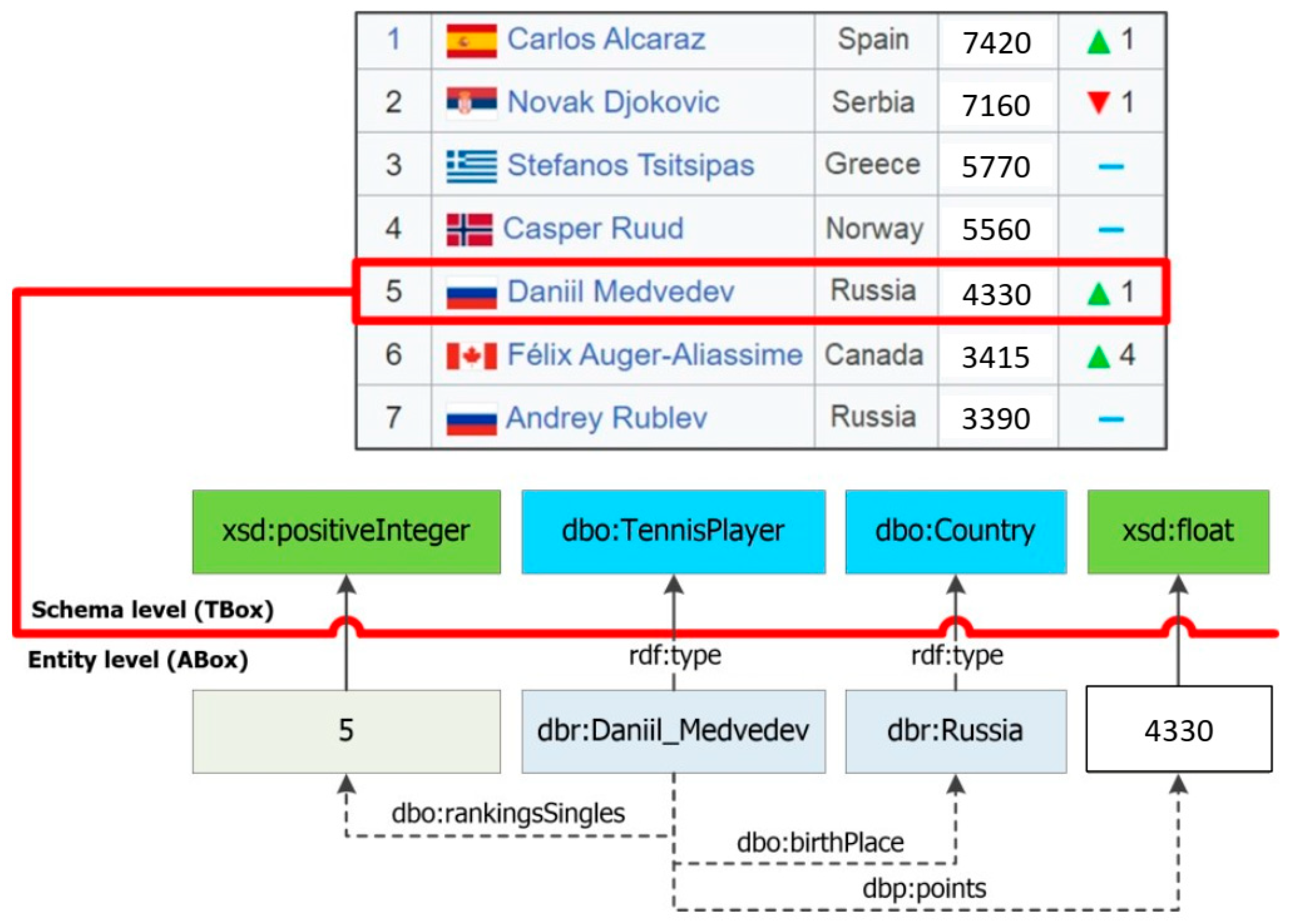
Stage 7. Entity extraction. At the last stage, a row-to-fact extraction is carried out based on defined annotations for columns and relationships between them. This stage is performed only for those cells whose annotations were not defined at Stage 4. A specific entity with a reference (rdf:type) to a relevant class is extracted for each cell of a subject column. This entity is associated with other entities or literals that are extracted from named entities and literal columns in the same row. In this case, a defined property between columns is set as the target relationship for such an association. It should be noted that the entity extraction algorithm uses an already defined ontology schema and does not identify new relationships.
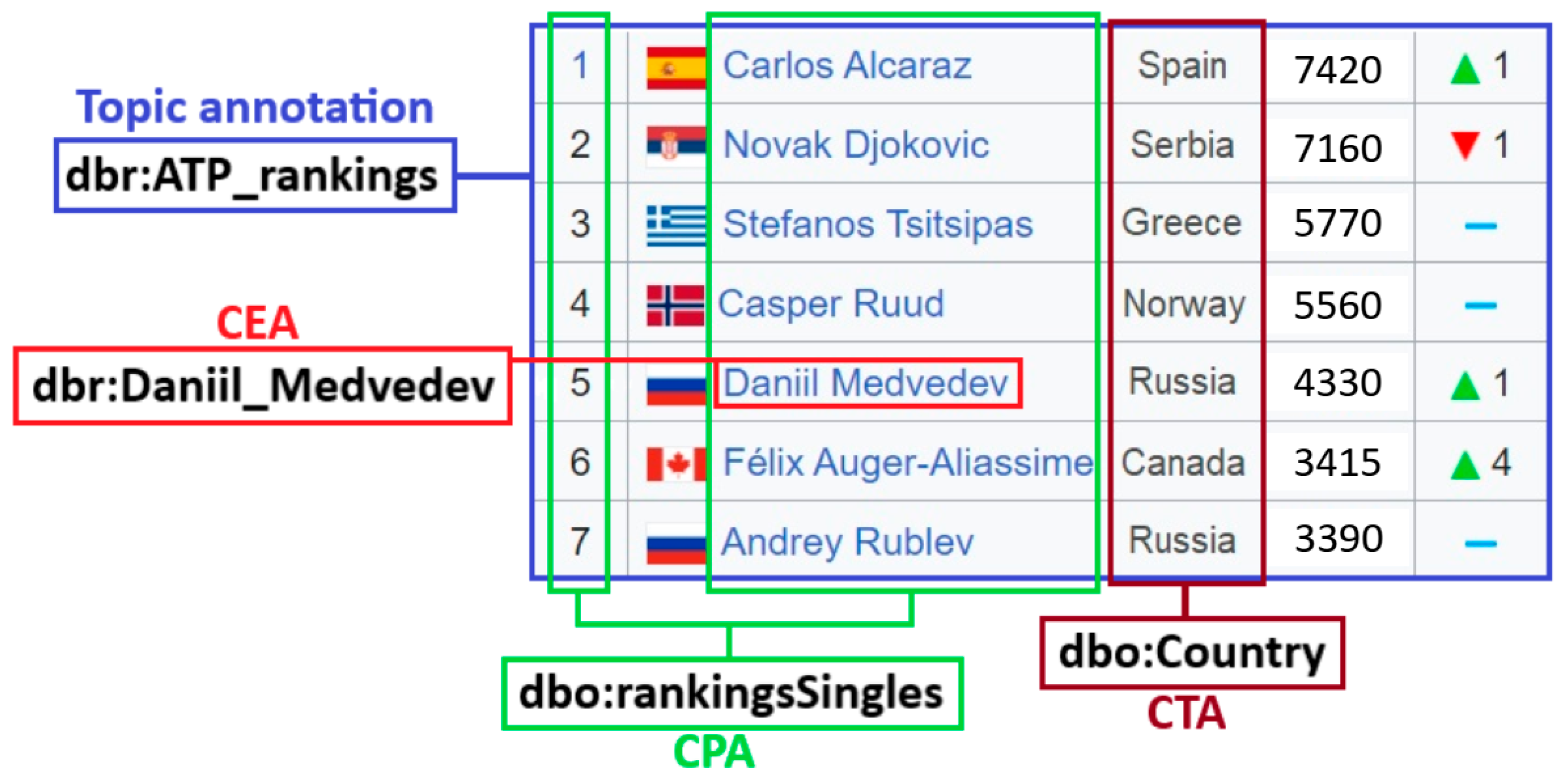
Thus, the RDF triples that contain extracted, specific entities and their properties (facts) are generated at the output. An example of row-to-fact extraction for annotated tabular data with the rating of tennis players “ATP rankings (singles) as of 20 March 2023” is presented in Figure 3. The entities extracted in this way can populate a target knowledge graph or ontology schema at the assertion level (ABox level).

4. Implementation

The proposed approach is implemented in the form of a web-based tool called TabbyLD2 [74,75]. This tool is written in Python and has a client-server architecture, as shown in Figure 4. TabbyLD2 includes the main modules:
  • Web table scraper searches for web tables by keywords and extracts them in JSON format from the archive of PubMed biomedical publications [76] and Wikipedia articles, which allows one to generate test datasets;
  • Table parser provides import and transformation of source tables from CSV, MS Excel (XLSX), or JSON format into an object table model implemented in Python;
  • Data cleaner provides tabular data cleaning;
  • Atomic column recognizer implements the stages of atomic column classification and subject column identification;
  • Semantic annotator is the main software module that links tabular data with entities, classes, and properties from a target knowledge graph (e.g., DBpedia) or an ontology schema;
  • Entity generator extracts specific entities (facts) from the cells of the annotated table and serializes them as RDF triplets;
  • Interaction module provides interaction with a target knowledge graph or an ontology schema. In particular, it supports interaction with DBpedia through the DBpedia SPARQL Endpoint [65] and DBpedia Lookup [66] services in order to obtain candidate sets of entities, classes, datatypes, and properties. This module also provides filling a target knowledge graph or an ontology schema with missing extracted facts in the form of RDF triplets;
  • Control module provides access to all functions of table processing. The module supports two modes of operation: it operates in console mode and as a web server that uses an open REST API based on the Flask micro-framework [77]. The second mode allows third-party services to access individual functions of the developed software.
We have also developed a client application (demo) called TabbyLD2-Client [78] on the PHP/Yii2 framework with a graphical user interface to support non-programming users (e.g., domain experts, data analysts, and knowledge engineers). This client application provides the following main functions:
  • import tables in CSV format;
  • classify columns into named entities and literal types and identify a subject column;
  • annotate cells, columns, and relations between columns;
  • viewing imported tabular data and the results of its preprocessing;
  • change table annotations, i.e., the user can select the necessary entity, class, or property from a set of found candidates (if he is not satisfied with automatically defined annotations);
  • generate RDF triplets based on annotated tabular data.
Thus, the developed tool supports both automatic annotation of table elements and manual refinement of the received annotations. The tool can also extract source tables from Wikipedia articles and the PubMed archive [17], which allows one to generate test datasets.

5. Experimental Evaluation

In this section, we present an experimental evaluation of the proposed approach. The purpose of our experiments is to show the applicability of our approach and tools for STI tasks.

5.1. Datasets

Several datasets were proposed to evaluate STI approaches. We selected the T2Dv2 Gold Standard (T2D) [79] as the main dataset for evaluating our approach and tool because of its wide application for testing the performance of table annotating methods (this dataset was specially created for STI tasks). The dataset is based on the Web Data Commons project and uses DBpedia as a target knowledge graph for table annotation. T2D consists of manually annotated row-to-instance, attribute-to-property, and table-to-class correspondences between 779 web tables and DBpedia version 2014. This dataset is the second version of the gold standard, plus negative examples. Web tables from T2D are presented in JSON format and cover different topics, including places, works, and people. A table from this dataset has, on average, 84 rows and 5 columns. There are a total of 411 columns in the dataset. Verification files contain references to 755 classes and 26,106 entities.
The SemTab challenge (Semantic Web Challenge on Tabular Data to Knowledge Graph Matching) collocated with the International Semantic Web Conference (ISWC) from 2019 to 2023 provides the largest datasets. In particular, the Tough Tables (2T) dataset [80] is introduced into SemTab 2020 to increase complexity. 2T consists of 180 specially designed tables that simulate various difficulties: a large number of rows to evaluate the performance, non-web tables, and artificially added misspellings and ambiguities. Tables from this dataset are presented in CSV format. A table from this dataset has an average of 1080 rows and 5 columns. We selected this dataset as an additional dataset for evaluating the proposed approach and tool. The main motivation for choosing this dataset is the possibility of comparison with competing approaches developed within the SemTab challenge, since it has been used in the competition for a long time (three years).

5.2. Evaluation Metrics

Traditionally, STI approaches are evaluated using the information retrieval metrics: Accuracy, Precision, Recall, and F1 score. The SemTab challenge defined a number of such metrics to evaluate different STI tasks, in particular CEA, CTA, and CPA [25]. However, the CTA task is a special case since a given semantic type (class) and its parents can all be correct when determining the category of an entity or of a group of entities in a table column. Therefore, the Average Hierarchical score (AH) and Average Perfect score (AP) are proposed and should take into account the taxonomy (hierarchy) of classes in the DBpedia knowledge graph [59].
We used metrics such as Precision, Recall, and F1 score to evaluate the CEA task [81]:
Precision = CA/A, Recall = CA/C,
F1 = (2 × Precision × Recall)/(Precision + Recall)
where CA is a number of correctly annotated cells; A is a number of annotated cells; C is a total number of cells.
We used AH and AP metrics to evaluate the CTA task [82]:
AH = (P + 0.5 × O + W)/T, AP = P/(P + O + W),
where P denotes perfect annotations involving the most fine-grained classes in the hierarchy that also appear in the ground truth; O is okay annotations involving the super-classes of perfect classes (excluding very generic top classes like owl:Thing); W is incorrect annotations (not in the ground truths); T denotes all columns for annotation.
In addition to the main scores for the CEA and CTA tasks, we used a well-known measure such as accuracy to obtain an experimental evaluation for atomic column classification:
Accuracy = CC/NC
where CC is a number of correctly typed columns into the named entity and literal; NC is a total number of columns in a source table.
We also calculated the accuracy of the subject column identification. If a subject column in a source table is defined correctly, then the accuracy is one; otherwise, the accuracy is zero.

5.3. Results and Discussion

The evaluation results for the stages of atomic column classification and subject column identification are presented in Table 5.
Note that the evaluation for subject column identification was not performed on the 2T dataset because there is no information on the basic truths for this task in the verification files. In general, the evaluation performed is high, which reflects the relevance of the proposed methods. However, a comprehensive comparison with competing approaches can be difficult because authors usually skip this stage, focusing only on STI tasks. Consequently, only the results obtained for the stage of subject column identification could be compared with three analogs: TAIPAN [32] (0.54), TableMiner+ [33] (0.87), and MantisTable [36] (0.98). Thus, our approach turned out to be better than TAIPAN and TableMiner +, but slightly inferior to MantisTable.
The evaluation results for the CEA task are presented in Table 6.
We performed a detailed experiment with our methods for the CEA task on the T2D dataset. In particular, we carried out separate evaluations for the developed heuristics and found out that the best option is the aggregation of all four heuristics. We found a significant number of errors and inconsistencies in the verification T2D files, which affected the evaluation received. Moreover, a candidate search step was also evaluated (whether there are relevant entities in a set of candidates). We determined that Recall cannot exceed 0.902. Thus, not only a disambiguation step but also a candidate search step can be improved further.
We performed a comparison of the evaluation results for the T2D dataset with competing solutions for the CEA task (see Table 7). Our results turned out to be better than some well-known analogues based on matching ontologies: LogMap [83], PARIS [84], and Blocking [85]. The efficiency of the proposed approach is close to the well-known analogues based on entity lookup techniques: FactBase Lookup [29], T2K Match [31], and TableMiner+ [33].
We also performed a comparison of evaluation results for the 2T dataset with some competing approaches participating in the SemTab-2021 competition. In particular, our results turned out to be better than the evaluation results for such tools as MAGIC [38] and Kepler-aSI [39] (F1 < 0.2). At the same time, TabbyLD2 performs as well as JenTab [40] (F1 = 0.6), but its performance is less efficient than that of the competition leader, DAGOBAH [41] (F1 = 0.9).
The evaluation results for the CTA task on the T2D and 2T datasets are presented in Table 8 and Table 9, respectively. We carried out complex experiments both with separate column annotation methods and with the aggregated method. Moreover, we also performed a comparison of evaluation results with competing approaches, such as ColNet [43], Sato [45], and Doduo [47]. In this case, we used only the basic version of the ColNet framework. A total of 169 customized binary CNN classifiers corresponding to each candidate class from DBpedia were trained for the T2D dataset. We used default settings for the Sato framework and already trained models on the WebTables corpus from the VizNet project. For Doduo, we also used a Turl-model that had been trained on the WikiTables dataset. At the same time, the mapping of concepts from Freebase into DBpedia classes to check the resulting annotations was done manually.
Thus, the performed AH and AP scores on the T2D dataset for our baseline solution are significantly higher than those of all three analogues separately. In particular, ColNet is based on the CEA results, which are not exact and need to be improved. Sato annotates columns with a set of 78 semantic types taken from DBpedia. These types are formed by training Sato models and are therefore well suited only for tabular data from the WebTables corpus or similar tables. Moreover, the verification of T2D files contains only classes as target annotations for columns, while there are only 24 classes and 54 properties (owl:DatatypeProperty and owl:ObjectProperty) among Sato’s semantic types. Doduo contains more semantic types than Sato, but the same problem still persists. The performed AH and AP scores on the 2T dataset for our baseline solution are significantly higher than those of Sato but slightly inferior to Doduo. In both cases, the aggregate method gave the best result.
The execution time of the baseline solution and the CNN-based column class prediction method (ColNet) was more than a day (1767 min) for the T2D dataset and about seven days (10,704 min) for the 2T dataset. Such a large execution time includes table preprocessing and solving the CEA task, which is quite resource-demanding since it requires a large number of SPARQL queries to a target knowledge graph. At the same time, Sato and Doduo approaches showed acceptable execution times, in particular, 17 min (T2D) and 34 min (2T) for Sato and 9 min (T2D) and 17 min (2T) for Doduo.
Thus, it is necessary to use the aggregated method to achieve the best result when solving the CTA task. However, the approach based on pre-trained language models that solve the problem in a reasonable time is still promising, even though it is slightly inferior in accuracy. Besides, if we carry out the additional training stage, then this approach will derive even better results.
It should be noted that all weighting factors for obtaining the final scores in the CEA and CTA tasks were set to 1, because the task was also to compare the proposed method of table annotation with others without additional adjustment to a specific dataset.
Table 10 shows a comparison of the qualitative indicators with the closest works [26,27,28,29,30,31,32,33,35,36,37,40,41,42,43,44,45,47,48,49,50]. We have grouped all existing methods into two classes: heuristic methods and deep-learning-based methods (e.g., using Deep Neural Networks (DNN) or BERT models). The first class includes techniques based on iterative algorithms, lookup services, and feature-based solutions. The second class of methods includes more modern solutions based on Deep Neural Networks (DNN) or pre-trained language models (e.g., BERT). At the same time, the “+” and “–” signs represent the availability and absence of a certain function or capability. For example, the “GUI” column indicates the presence of a graphical user interface for the corresponding software solution.
The proposed approach has its advantages; for example, it covers the solution to all STI problems and also allows one to extract specific entities from annotated tables. It should also be noted that the developed tool can be configured for any target knowledge graph, both cross-domain and domain-specific (enterprise). However, the proposed approach has its limitations and disadvantages. In particular, an important limitation is the use of only relational tables as input. In [86], we made the first attempt to solve this problem by representing arbitrary tables in a canonical form. In the future, we plan to expand processing to other types of tables (e.g., vertical, horizontal, and matrix). We also plan to further explore the prospect of using deep machine learning methods based on pre-trained language models to build a complete model for table understanding.

6. Case Study

In this section, we present the results of the application of our approach for modeling and filling knowledge graphs in some domains: industrial safety inspection, labor market analysis, and analysis of university activities.

6.1. Industrial Safety Inspection

The reliability and safety of industrial facilities is one of the domains that require processing a large amount of poorly structured data. The safety provision problem in industrial facilities remains a relevant issue in many industries. It is mainly associated with the degradation and aging of technical equipment, which are ahead of the pace of modernization and replacement. This is especially true for long-running technical equipment at oil refineries, petrochemical plants, and chemical plants. Such technical equipment requires periodic assessments of its technical condition. The assessment is carried out by means of technical diagnostics and examination in order to determine potentially dangerous elements and components, with subsequent decision-making to eliminate failures. The technical condition assessment of such facilities is carried out as part of the Industrial Safety Inspection (ISI) procedure [87]. In most cases, the ISI procedure consists of the following main stages: planning works for the ISI; analysis of technical documentation; forming a map of initial data; development of an ISI program; technical diagnostics; analysis (including interpretation) of diagnostic results; calculation of durability and residual life; and making decisions for the repair. The input data and the results of each task are fixed in the reports. This information is not structured enough for computer-aided processing. Mostly, it is stored on electronic media and has a form that can be processed at best only with text editors. In addition, the existing requirements (standards) [88] regulate the content of these documents only at the general level. At the same time, ISI reports contain heterogeneous information in the form of texts, tables, charts, and graphs. Herewith, tables provide the most structured and formalized representation of domain entities. In most cases, such tables contain some domain semantics and, accordingly, are the most promising source for the computer-aided extraction of information.
The purpose of this case study was to fill out an ontology schema of a domain knowledge graph that describes measurement results of technical states of petrochemical equipment for the ISI tasks with specific entities (facts) extracted from tables from an open dataset, “ISI-167E: Entity Spreadsheet Tables” [89]. This dataset was formed on the basis of ISI reports that were provided by our customer. The ISI-167E dataset contains 167 relational tables presented in the CSV format. Fragments of tables describing measurement results for a storage tank from the ISI-167E dataset are presented in Figure 5.
All tables from the ISI-167E dataset were semantically annotated using TabbyLD2 and a target domain ontology schema. This schema describes the ISI field and was created manually by domain experts [90] using the conceptual (cognitive) modeling tool, in particular, the IHMC CmapTools software [91], and the ontological modeling tool (Protégé [92]). A fragment of this schema is presented in Figure 6.
The annotation of tables was done automatically. However, the CEA stage was skipped because there were no specific entities in our domain-specific knowledge graph or in the cross-domain knowledge graph (DBpedia). Therefore, a heading similarity, a NER-based similarity, a BERT-based column class prediction, and a coherence algorithm were used for the CTA task. In this case, the weighting factors for the first two similarity methods were set to 2, and the method based on the BERT model was set to 1. This was done because the BERT model was not tuned for this dataset (the default Sato model was used). Note that some annotations for columns and relationships between them were detected incorrectly. Those annotations were refined manually by domain experts. In total, 153 classes and about 500 properties were defined. A screenshot of the TabbyLD2-Client application with the defined annotations for the “Storage tank” table is presented in Figure 7. The annotations themselves are displayed in square brackets in the header. 1036 specific unique entities (facts) were extracted from table rows using the defined columns and relationship annotations. Thus, our target ontology schema at the assertion level (ABox) was populated with these entities, and, as a result, a domain-specific knowledge graph for the ISI procedure was obtained.
We conducted additional experiments that allowed us to determine the accuracy of the automatic stages of table processing.
The accuracy from (17) was used as the main measure to perform the experimental evaluation for the atomic column classification. As a result, we obtained an accuracy of 0.92.
We used the accuracy to perform an experimental evaluation at the CTA stage:
accuracycta = CAC/CN,
where CAC is a number of correctly annotated columns (perfect annotations); CN is a total number of columns in a source table.
Experiments with both separate heuristic methods and a BERT-based column class prediction method (sato and turl models) were performed. The correctness of column annotations was determined by domain experts. The evaluation results are presented in Table 11.
We also used accuracy to perform experimental evaluation at the entity extraction stage:
accuracyee = NCE/(NR × NC),
where NCE is a number of correctly extracted specific entities; NR is a total number of rows in a source table; and NC is a number of named entity columns in a source table. As a result, accuracy = 0.97.
Thus, a domain knowledge graph was formed and used for a decision support system for ISI tasks, in particular, the diagnosis and assessment of the technical states of petrochemical equipment and technological complexes.

6.2. Labor Market Analysis

The proposed approach was used as part of a case study conducted for the Ivannikov Institute for System Programming of the Russian Academy of Sciences (ISP RAS). The problem of the automated population of domain-specific knowledge graphs for the Talisman framework [93] was solved. This framework combines Big Data software components and uses technologies developed by ISP RAS, such as Dedoc (a document structure extraction system) and Texterra (a platform for extracting semantics from text), as its main services. We used the TabbyLD2 tool as a plugin in the Talisman Information Extraction (TIE) software. This plugin provides automated semantic annotation of tables contained in the Talisman document in the form of the TDM (Talisman Document Model) and extraction of new facts from the semantically annotated tabular data.
We applied the plugin to analyze the labor market (open vacancies in the IT industry) in Irkutsk Oblast. Irkutsk Oblast is a federal subject of the Russian Federation located in southeastern Siberia. An ontology schema of target knowledge graphs for this field was developed within the Talisman framework. This schema was also created manually by analysts from the ISP RAS. The developed ontology schema describes vacancies, persons, companies, educational institutions, and skills, and it is shown in Figure 8. A knowledge graph has the form of a semantically directed graph (Label Property Graph) and is accessed using the GraphQL interface [94].
We used open data on the Web to search for information about vacancies in Irkutsk Oblast. We processed such Web resources as hh.ru, superjob.ru, rabota.ru, avito.ru, zarplata.ru, and irk.rosrabota.ru, as well as a databank of vacancies in Irkutsk Oblast [95] and the Irkutsk Regional Multifunctional Center for Public Services [96]. We manually selected IT vacancies that appeared in the last two months. Thus, four Talisman documents containing eight aggregated tables were created. Each table contained more than 200 vacancies.
Semantic annotation for these tables was done automatically using the plugin. However, only the CTA stage was completed. In particular, we used the baseline solution (majority voting and heading similarity methods with weighting factors equal to 1) with the coherence algorithm. In total, 1678 new specific entities (facts) were extracted from the tables. A target knowledge graph was populated with these facts.
We used the accuracy from (18) as the main measure to perform the experimental evaluation at the CTA stage. The evaluation results are presented in Table 12. The evaluations performed showed the prospects of the proposed approach.

6.3. Analysis of the Activities of Universities

Let’s consider an additional practical task for the Talisman framework, which consisted of analyzing the activities of universities over a certain period. For this purpose, we have developed a domain-specific knowledge graph based on various documents and tables extracted from the Web. In particular, we have created an open set of tabular data called “wiki-UKU-49: United Kingdom Universities from Wikipedia” [97]. This dataset contains tables describing the main concepts and relationships in the field of education in the United Kingdom (e.g., educational institution, student political society, foundation date, university status, territory, endowment, location, and persons). Source tables were obtained by automatically extracting them from Wikipedia articles in the “universities in the United Kingdom” category. These tables were manually processed, and 49 relational tables were selected for this dataset. Each table represents a set of entities of the same type. Selected tables are presented in both CSV and JSON formats. This dataset also contains an additional text file with a brief description of the tables.
An ontology schema of a target knowledge graph that describes educational institutions in the United Kingdom was also created manually by analysts from the ISP RAS in the form of a semantically directed graph (Label Property Graph). Figure 9 shows a fragment of a target ontology schema, which describes the main concepts (classes) of the educational institution and its properties (relationships).
The process of semantic annotation for tables from the “wiki-UKU-49: United Kingdom Universities from Wikipedia” dataset based on the developed ontology schema was done automatically using our tool. However, just like for the previous case study, the CTA stage was completed only using majority voting and heading similarity methods (weighting factors for these methods are 1) and the coherence algorithm. For the CPA stage, a set of candidate properties was automatically formed based on a target ontology schema (see Figure 9) for linking a subject column between all other columns in a source table. As a result, 2940 new specific entities (facts) were extracted from the tables and added to a target knowledge graph. For example, 45 entities denoting student unions and 45 entities denoting different colleges and universities were extracted from the table “List of UK student political societies”.
We used the accuracy from (18) as the main measure to perform the experimental evaluation at the CTA stage (separately for named entities and literal columns). We also used accuracy to perform the experimental evaluation of the annotation of relationships between columns:
accuracycpa = CP/PN,
where CP is the number of correctly annotated relationships (ontology properties) between columns (perfect annotations); PN is the total number of annotated relationships between columns.
As a result, accuracycta = 0.82 and accuracycpa = 0.53. The evaluations performed showed quite acceptable results.

7. Conclusions

The integration of methods for the semantic interpretation of tabular data and the development of knowledge graphs is becoming an area of active scientific research. Existing approaches have limitations both for the tabular layouts and the domains covered. Moreover, almost all of them target programmers.
In this paper, we propose a hybrid approach for the semantic interpretation of tables and entity extraction from semantically annotated tabular data as a first step toward building a universal solution for understanding table information. The proposed approach was implemented as a web-based tool (TabbyLD2 [74,75]) to quickly fill domain-specific knowledge graphs with specific entities (facts) extracted from the table rows. This tool has an intuitive graphical user interface and has already been used to solve practical, poorly formalized tasks. The experiments and case studies performed have shown the prospects of using our approach and tool.

Author Contributions

Conceptualization and methodology, N.D. and A.Y.; software, N.D.; validation, N.D. and A.Y.; writing—original draft preparation, N.D.; data curation, N.D. and A.Y. All authors have read and agreed to the published version of the manuscript.

Funding

This work was supported by the Council for Grants of the President of the Russian Federation (Grant No. SP-978.2022.5) and the Ministry of Education and Science of the Russian Federation (Project No. 121030500071-2).

Data Availability Statement

Not applicable.

Conflicts of Interest

The authors declare no conflict of interest.

References

  1. Hogan, A.; Blomqvist, E.; Cochez, M.; d’Amato, C.; Melo, G.D.; Gutierrez, C.; Gayo, J.E.L.; Kirrane, S.; Neumaier, S.; Polleres, A.; et al. Knowledge Graphs. ACM Comput. Surv. 2021, 54, 1–37. [Google Scholar] [CrossRef]
  2. Ji, S.; Pan, S.; Cambria, E.; Marttinen, P.; Yu, P.S. A Survey on Knowledge Graphs: Representation, Acquisition and Applications. IEEE Trans. Neural Netw. Learn. Syst. 2021, 33, 494–514. [Google Scholar] [CrossRef] [PubMed]
  3. Singhal, A. Introducing the Knowledge Graph: Things, Not Strings. Google Blog. Available online: https://www.blog.google/products/search/introducing-knowledge-graph-things-not/ (accessed on 7 June 2023).
  4. Peroni, S.; Shotton, D.M.; Vitali, F. One Year of the OpenCitations Corpus—Releasing RDF-Based Scholarly Citation Data into the Public Domain. In Proceedings of the 16th International Semantic Web Conference (ISWC’2017), Vienna, Austria, 21–25 October 2017. [Google Scholar]
  5. Iana, A.; Jung, S.; Naeser, P.; Birukou, A.; Hertling, S.; Paulheim, H. Building a Conference Recommender System Based on SciGraph and WikiCFP. In Proceedings of the Semantic Systems. The Power of AI and Knowledge Graphs: 15th International Conference, SEMANTiCS 2019, Karlsruhe, Germany, 9–12 September 2019; 11702, pp. 117–123. [Google Scholar]
  6. Färber, M. The Microsoft Academic Knowledge Graph: A Linked Data Source with 8 Billion Triples of Scholarly Data. In Proceedings of the 18th International Semantic Web Conference (ISWC’2019), Auckland, New Zealand, 26–30 October 2019. [Google Scholar]
  7. Stadler, C.; Lehmann, J.; Höffner, K.; Auer, S. LinkedGeoData: A core for a web of spatial open data. Semant. Web J. 2012, 3, 333–354. [Google Scholar] [CrossRef]
  8. Callahan, A.; Cruz-Toledo, J.; Ansell, P.; Dumontier, M. Bio2RDF Release 2: Improved Coverage, Interoperability and Provenance of Life Science Linked Data. In Proceedings of the Semantic Web: Semantics and Big Data, 10th International Conference (ESWC 2013), Montpellier, France, 26–30 May 2013. [Google Scholar]
  9. Raimond, Y.; Ferne, T.; Smethurst, M.; Adams, G. The BBC World Service Archive prototype. J. Web Semant. 2014, 27–28, 2–9. [Google Scholar] [CrossRef]
  10. Tiwari, S.; Al-Aswadi, F.N.; Gaurav, D. Recent trends in knowledge graphs: Theory and practice. Soft Comput. 2021, 25, 8337–8355. [Google Scholar] [CrossRef]
  11. Xiaoxue, L.; Xuesong, B.; Longhe, W.; Bingyuan, R.; Shuhan, L.; Lin, L. Review and trend analysis of knowledge graphs for crop pest and diseases. IEEE Access 2019, 7, 62251–62264. [Google Scholar] [CrossRef]
  12. Lehmberg, O.; Ritze, D.; Meusel, R.; Bizer, C. A large public corpus of web tables containing time and context metadata. In Proceedings of the 25th International Conference Companion on World Wide Web, Montréal, QC, Canada, 11–15 April 2016. [Google Scholar]
  13. Burdick, D.; Danilevsky, M.; Evfimievski, A.V.; Katsis, Y.; Wang, N. Table extraction and understanding for scientific and enterprise applications. Proc. VLDB Endow. 2020, 13, 3433–3436. [Google Scholar] [CrossRef]
  14. Martinez-Rodriguez, J.L.; Hogan, A.; Lopez-Arevalo, I. Information Extraction meets the Semantic Web: A Survey. Semantic Web. 2020, 11, 255–335. [Google Scholar] [CrossRef]
  15. OWL 2 Web Ontology Language Document Overview (Second Edition). Available online: https://www.w3.org/TR/owl2-overview/ (accessed on 7 June 2023).
  16. Resource Description Framework (RDF). Available online: https://www.w3.org/RDF/ (accessed on 7 June 2023).
  17. Ehrlinger, L.; Woß, W. Towards a Definition of Knowledge Graphs. SEMANTiCS 2016, 48, 2. [Google Scholar]
  18. Gruber, T.R. A Translation Approach to Portable Ontology Specifications. Knowl. Acquis. 1993, 5, 199–220. [Google Scholar] [CrossRef]
  19. Villazon-Terrazas, B.; Garcia-Santa, N.; Ren, Y.; Srinivas, K.; Rodriguez-Muro, M.; Alexopoulos, P.; Pan, J.Z. Construction of Enterprise Knowledge Graphs (I). In Exploiting Linked Data and Knowledge Graphs in Large Organisations; Pan, J.Z., Vetere, G., Gomez-Perez, J.M., Wu, H., Eds.; Springer: Cham, Switzerland, 2017; pp. 87–116. [Google Scholar]
  20. Ré, C.; Sadeghian, A.A.; Shan, Z.; Shin, J.; Wang, F.; Wu, S.; Zhang, C. Feature engineering for knowledge base construction. IEEE Data Eng. Bull. 2014, 37, 26–40. [Google Scholar]
  21. Balog, K. Populating knowledge bases. Entity-Oriented Search INRE 2018, 39, 189–222. [Google Scholar]
  22. Zhang, S.; Balog, K. Web table extraction, retrieval, and augmentation: A survey. ACM Trans. Intell. Syst. Technol. 2020, 11, 1–35. [Google Scholar] [CrossRef]
  23. Bonfitto, S.; Casiraghi, E.; Mesiti, M. Table understanding approaches for extracting knowledge from heterogeneous tables. Wiley Interdiscip. Rev. Data Min. Knowl. Discov. 2021, 11, e1407. [Google Scholar] [CrossRef]
  24. Shigarov, A. Table understanding: Problem overview. Wiley Interdiscip. Rev. Data Min. Knowl. Discov. 2022, 13, e1482. [Google Scholar] [CrossRef]
  25. Liu, J.; Chabot, Y.; Troncy, R.; Huynh, V.-P.; Labbé, T.; Monnin, P. From tabular data to knowledge graphs: A survey of semantic table interpretation tasks and methods. J. Web Semant. 2023, 76, 100761. [Google Scholar] [CrossRef]
  26. Limaye, G.; Sarawagi, S.; Chakrabarti, S. Annotating and Searching Web Tables Using Entities, Types and Relationships. Proc. VLDB Endow. 2010, 3, 1338–1347. [Google Scholar] [CrossRef]
  27. Mulwad, V.; Finin, T.; Syed, Z.; Joshi, A. Using linked data to interpret tables. In Proceedings of the First International Conference on Consuming Linked Data, Aachen, Germany, 8 November 2010. [Google Scholar]
  28. Venetis, P.; Halevy, A.; Madhavan, J.; Pasca, M.; Shen, W.; Wu, F.; Miao, G.; Wu, C. Recovering Semantics of Tables on the Web. Proc. VLDB Endow. 2011, 4, 528–538. [Google Scholar] [CrossRef]
  29. Efthymiou, V.; Hassanzadeh, O.; Rodriguez-Muro, M.; Christophides, V. Matching web tables with knowledge base entities: From entity lookups to entity embeddings. In Proceedings of the 16th International Semantic Web Conference (ISWC’2017), Vienna, Austria, 21–25 October 2017. [Google Scholar]
  30. Bhagavatula, C.S.; Noraset, T.; Downey, D. TabEL: Entity Linking in Web Tables. In Proceedings of the 14th International Semantic Web Conference (ISWC’2015), Bethlehem, PA, USA, 11–15 October 2015. [Google Scholar]
  31. Ritze, D.; Bizer, C. Matching Web Tables To Dbpedia—A Feature Utility Study. In Proceedings of the 20th International Conference on Extending Database Technology (EDBT), Venice, Italy, 21–24 March 2017. [Google Scholar]
  32. Ermilov, I.; Ngomo, A.-C.N. TAIPAN: Automatic Property Mapping for Tabular Data. In Proceedings of the 20th International Conference on European Knowledge Acquisition Workshop (EKAW), Bologna, Italy, 19–23 November 2016. [Google Scholar]
  33. Zhang, Z. Effective and Efficient Semantic Table Interpretation using TableMiner+. Semant. Web 2017, 8, 921–957. [Google Scholar] [CrossRef]
  34. SemTab: Semantic Web Challenge on Tabular Data to Knowledge Graph Matching. Available online: https://www.cs.ox.ac.uk/isg/challenges/sem-tab/ (accessed on 7 June 2023).
  35. Kruit, B.; Boncz, P.; Urbani, J. Extracting novel facts from tables for knowledge graph completion. In Proceedings of the 18th International Semantic Web Conference (ISWC’2019), Auckland, New Zealand, 26–30 October 2019. [Google Scholar]
  36. Cremaschi, M.; Paoli, D.F.; Rula, A.; Spahiu, B. A fully automated approach to a complete Semantic Table Interpretation. Future Gener. Comput. Syst. 2020, 112, 478–500. [Google Scholar] [CrossRef]
  37. Nguyen, P.; Kertkeidkachorn, N.; Ichise, R.; Takeda, H. MTab: Matching Tabular Data to Knowledge Graph using Probability Models. In Proceedings of the 18th International Semantic Web Conference (ISWC’2019), Auckland, New Zealand, 26–30 October 2019. [Google Scholar]
  38. Steenwinckel, B.; Turck, F.D.; Ongenae, F. MAGIC: Mining an Augmented Graph using INK, starting from a CSV. In Proceedings of the 20th International Semantic Web Conference (ISWC’2021), Virtual Conference, 24–28 October 2021. [Google Scholar]
  39. Baazouzi, W.; Kachroudi, M.; Faiz, S. Kepler-aSI at SemTab. In Proceedings of the 20th International Semantic Web Conference (ISWC’2021), Virtual Conference, 24–28 October 2021. [Google Scholar]
  40. Abdelmageed, N.; Schindler, S. JenTab Meets SemTab 2021′s New Challenges. In Proceedings of the 20th International Semantic Web Conference (ISWC’2021), Virtual Conference, 24–28 October 2021. [Google Scholar]
  41. Huynh, V.-P.; Liu, J.; Chabot, Y.; Deuzé, F.; Labbé, T.; Monnin, P.; Troncy, R. DAGOBAH: Table and Graph Contexts For Efficient Semantic Annotation Of Tabular Data. In Proceedings of the 20th International Semantic Web Conference (ISWC’2021), Virtual Conference, 24–28 October 2021. [Google Scholar]
  42. Xie, J.; Lu, Y.; Cao, C.; Li, Z.; Guan, Y.; Liu, Y. Joint Entity Linking for Web Tables with Hybrid Semantic Matching. In Proceedings of the International Conference on Computational Science, Amsterdam, The Netherlands, 3–5 June 2020. [Google Scholar]
  43. Chen, J.; Jimenez-Ruiz, E.; Horrocks, I.; Sutton, C. ColNet: Embedding the semantics of web tables for column type prediction. In Proceedings of the AAAI Conference on Artificial Intelligence, Honolulu, HI, USA, 27 January 2019. [Google Scholar]
  44. Hulsebos, M.; Hu, K.; Bakker, M.; Zgraggen, E.; Satyanarayan, A.; Kraska, T.; Demiralp, Ç.; Hidalgo, C. Sherlock: A Deep Learning Approach to Semantic Data Type Detection. In Proceedings of the 25th ACM SIGKDD International Conference on Knowledge Discovery & Data Mining (KDD’19), Anchorage, AK, USA, 4–8 August 2019. [Google Scholar]
  45. Zhang, D.; Suhara, Y.; Li, J.; Hulsebos, M.; Demiralp, Ç.; Tan, W.-C. Sato: Contextual Semantic Type Detection in Tables. Proc. VLDB Endow. 2020, 13, 1835–1848. [Google Scholar] [CrossRef]
  46. Devlin, J.; Chang, M.-W.; Lee, K.; Toutanova, K. BERT: Pre-training of Deep Bidirectional Transformers for Language Understanding. In Proceedings of the 17th Annual Conference of the North American Chapter of the Association for Computational Linguistics: Human Language Technologies (NAACL-HLT 2019), Minneapolis, MN, USA, 2–7 June 2019. [Google Scholar]
  47. Suhara, Y.; Li, J.; Li, Y.; Zhang, D.; Demiralp, Ç.; Chen, C.; Tan, W.-C. Annotating Columns with Pre-trained Language Models. In Proceedings of the 2022 International Conference on Management of Data (SIGMOD’22), Philadelphia, PA, USA, 12–17 June 2022. [Google Scholar]
  48. Deng, X.; Sun, H.; Lees, A.; Wu, Y.; Yu, C. TURL: Table Understanding through Representation Learning. Proc. VLDB Endow. 2020, 14, 307–319. [Google Scholar] [CrossRef]
  49. Trabelsi, M.; Cao, J.; Heflin, J. SeLaB: Semantic Labeling with BERT. In Proceedings of the International Joint Conference on Neural Networks (IJCNN), Shenzhen, China, 18–22 July 2021. [Google Scholar]
  50. Yin, P.; Neubig, G.; Yih, W.; Riedel, S. TaBERT: Pretraining for Joint Understanding of Textual and Tabular Data. In Proceedings of the 58th Annual Meeting of the Association for Computational Linguistics, Online, 5–10 July 2020. [Google Scholar]
  51. Herzig, J.; Nowak, P.K.; Muller, T.; Piccinno, F.; Eisenschlos, J.M. TAPAS: Weakly Supervised Table Parsing via Pre-training. In Proceedings of the 58th Annual Meeting of the Association for Computational Linguistics, Online, 5–10 July 2020. [Google Scholar]
  52. Iida, H.; Thai, D.; Manjunatha, V.; Iyyer, M. TABBIE: Pretrained Representations of Tabular Data. In Proceedings of the 2021 Conference of the North American Chapter of the Association for Computational Linguistics: Human Language Technologies, Online, 6–11 June 2021. [Google Scholar]
  53. Wang, Z.; Dong, H.; Jia, R.; Li, J.; Fu, Z.; Han, S.; Zhang, D. TUTA: Tree-based Trans-formers for Generally Structured Table Pre-training. In Proceedings of the 27th ACM SIGKDD Conference on Knowledge Discovery & Data Mining (KDD’21), New York, NY, USA, 14–18 August 2021. [Google Scholar]
  54. Maguire, E.; Gonzalez-Beltran, A.; Whetzel, P.L.; Sansone, S.A.; Rocca-Serra, P. OntoMaton: A Bioportal powered ontology widget for Google Spreadsheets. Bioinformatics 2013, 29, 525–527. [Google Scholar] [CrossRef] [PubMed]
  55. González-Beltrán, A.; Maguire, E.; Sansone, S.A.; Rocca-Serra, P. linkedISA: Semantic representation of ISA-Tab experimental metadata. BMC Bioinform. 2014, 15, S4. [Google Scholar] [CrossRef] [PubMed]
  56. Vu, B.; Knoblock, C.A.; Szekely, P.; Pham, M.; Pujara, J. A Graph-Based Approach for Inferring Semantic Descriptions of Wikipedia Tables. In Proceedings of the 20th International Semantic Web Conference (ISWC’2021), Virtual Conference, 24–28 October 2021. [Google Scholar]
  57. De Vos, M.; Wielemaker, J.; Rijgersberg, H.; Schreiber, G.; Wielinga, B.; Top, J. Combining information on structure and content to automatically annotate natural science spreadsheets. Int. J. Hum.-Comput. Stud. 2017, 103, 63–76. [Google Scholar] [CrossRef]
  58. Wu, T.; Yan, S.; Piao, Z.; Xu, L.; Wang, R.; Qi, G. Entity Linking in Web Tables with Multiple Linked Knowledge Bases. In Proceedings of the 6th Joint International Semantic Technology Conference (JIST), Singapore, 2–4 November 2016. [Google Scholar]
  59. Bizer, C.; Lehmann, J.; Kobilarov, G.; Auer, S.; Becker, C.; Cyganiak, R.; Hellmann, S. Dbpedia—A Crystallization Point for the Web of Data. J. Web Semant. 2009, 7, 154–165. [Google Scholar] [CrossRef]
  60. ftfy: Fixes Text for You. Available online: https://pypi.org/project/ftfy/ (accessed on 7 June 2023).
  61. Stanford CoreNLP. Available online: https://stanfordnlp.github.io/CoreNLP/ (accessed on 7 June 2023).
  62. Duckling. Available online: https://github.com/facebook/duckling (accessed on 7 June 2023).
  63. Dateparser. Available online: https://dateparser.readthedocs.io/en/latest/ (accessed on 7 June 2023).
  64. SPARQL 1.1 Query Language. Available online: https://www.w3.org/TR/sparql11-query/ (accessed on 7 June 2023).
  65. DBpedia SPARQL Endpoint. Available online: https://dbpedia.org/sparql (accessed on 7 June 2023).
  66. DBpedia Lookup. Available online: https://lookup.dbpedia.org/index.html (accessed on 7 June 2023).
  67. Guan, N.; Song, D.; Liao, L. Knowledge graph embedding with concepts. Knowl.-Based Syst. 2019, 164, 38–44. [Google Scholar] [CrossRef]
  68. Ristoski, P.; Rosati, J.; Noia, T.D.; Leone, R.; Paulheim, H. RDF2Vec: RDF graph embeddings and their applications. Semant. Web 2019, 10, 721–752. [Google Scholar] [CrossRef]
  69. Portisch, J.; Hladik, M.; Paulheim, H. KGvec2go—Knowledge Graph Embeddings as a Service. In Proceedings of the Twelfth Language Resources and Evaluation Conference, Marseille, France, 11–16 May 2020. [Google Scholar]
  70. Le, Q.; Mikolov, T. Distributed Representations of Sentences and Documents. In Proceedings of the 31st International Conference on Machine Learning (PMLR), Beijing, China, 22–24 June 2014. [Google Scholar]
  71. ISO 4217—Currency Codes. Available online: https://www.iso.org/iso-4217-currency-codes.html (accessed on 31 August 2023).
  72. Hu, K.; Gaikwad, N.; Bakker, M.; Hulsebos, M.; Zgraggen, E.; Hidalgo, C.; Kraska, T.; Li, G.; Satyanarayan, A.; Demiralp, Ç. VizNet: Towards A Large-Scale Visualization Learning and Benchmarking Repository. In Proceedings of the 2019 CHI Conference on Human Factors in Computing Systems (CHI’19), Glasgow, Scotland, UK, 4–9 May 2019. [Google Scholar]
  73. XML Schema Part 2: Datatypes Second Edition. Available online: https://www.w3.org/TR/xmlschema-2/ (accessed on 7 June 2023).
  74. TabbyLD2. Available online: https://github.com/tabbydoc/tabbyld2 (accessed on 7 June 2023).
  75. Dorodnykh, N.O.; Yurin, A.Y. TabbyLD: A Tool for Semantic Interpretation of Spreadsheets Data. Commun. Comput. Inf. Sci. 2021, 1341, 315–333. [Google Scholar]
  76. PubMed. Available online: https://pubmed.ncbi.nlm.nih.gov/ (accessed on 7 June 2023).
  77. Flask. Available online: https://flask.palletsprojects.com/en/2.3.x/ (accessed on 7 June 2023).
  78. TabbyLD2-Client. Available online: https://github.com/tabbydoc/tabbyld2_client (accessed on 7 June 2023).
  79. T2Dv2 Gold Standard for Matching Web Tables to DBpedia. Available online: http://webdatacommons.org/webtables/goldstandardV2.html (accessed on 7 June 2023).
  80. Cutrona, V.; Bianchi, F.; Jimenez-Ruiz, E.; Palmonari, M. Tough tables: Carefully evaluating entity linking for tabular data. In Proceedings of the 19th International Semantic Web Conference (ISWC’2020), Athens, Greece, 2–6 November 2020. [Google Scholar]
  81. Cell-Entity Annotation (CEA) Challenge. Available online: https://www.aicrowd.com/challenges/semtab-2020/problems/cell-entity-annotation-cea-challenge (accessed on 7 June 2023).
  82. Column-Type Annotation (CTA) Challenge. Available online: https://www.aicrowd.com/challenges/semtab-2020/problems/column-type-annotation-cta-challenge (accessed on 7 June 2023).
  83. Jimenez-Ruiz, E.; Grau, B.C. LogMap: Logic-based and scalable ontology matching. In Proceedings of the 10th International Semantic Web Conference (ISWC’2011), Bonn, Germany, 23–27 October 2011. [Google Scholar]
  84. Suchanek, F.M.; Abiteboul, S.; Senellart, P. PARIS: Probabilistic alignment of relations, instances, and schema. Proc. VLDB Endow. 2012, 5, 157–168. [Google Scholar] [CrossRef]
  85. Christophides, V.; Efthymiou, V.; Stefanidis, K. Entity Resolution in the Web of Data; Springer: Cham, Switzerland, 2015. [Google Scholar]
  86. Dorodnykh, N.O.; Yurin, A.Y. Towards a universal approach for semantic interpretation of spreadsheets data. In Proceedings of the 24th Symposium on International Database Engineering & Applications (IDEAS’20), Seoul, Republic of Korea, 12–14 August 2020. [Google Scholar]
  87. Berman, A.F.; Nikolaichuk, O.A.; Yurin, A.Y.; Kuznetsov, K.A. Support of Decision-Making Based on a Production Approach in the Performance of an Industrial Safety Review. Chem. Pet. Eng. 2015, 50, 730–738. [Google Scholar] [CrossRef]
  88. Federal Law #116. Available online: http://www.consultant.ru/document/cons_doc_LAW_15234/ (accessed on 7 June 2023).
  89. ISI-167E: Entity Spreadsheet Tables. Available online: https://data.mendeley.com/datasets/3gjy46mx88/1 (accessed on 7 June 2023).
  90. Yurin, A.Y.; Dorodnykh, N.O.; Shigarov, A.O. Semi-Automated Formalization and Representation of the Engineering Knowledge Extracted From Spreadsheet Data. IEEE Access 2021, 9, 157468–157481. [Google Scholar] [CrossRef]
  91. IHMC CmapTools. Available online: https://cmap.ihmc.us/ (accessed on 7 June 2023).
  92. Protégé. Available online: https://protege.stanford.edu/ (accessed on 7 June 2023).
  93. TALISMAN (Tracking and Learning Insights from Social Media Analysis). Available online: https://talisman.ispras.ru/ (accessed on 7 June 2023).
  94. GraphQL. Available online: https://graphql.org/ (accessed on 7 June 2023).
  95. A Databank of Vacancies of Irkutsk Oblast. Available online: https://www.irkzan.ru/vacancy (accessed on 7 June 2023).
  96. Irkutsk Regional Multifunctional Center for Public Services. Available online: https://mfc38.ru/ (accessed on 7 June 2023).
  97. wiki-UKU-49: United Kingdom Universities from Wikipedia. Available online: https://data.mendeley.com/datasets/33v9tk6jjb/1 (accessed on 7 June 2023).
Figure 1. An example of main STI tasks for a table “ATP rankings (singles) as of 20 March 2023”.
Computation 11 00175 g001
Figure 2. The main stages of the approach.
Computation 11 00175 g002
Figure 3. An example of row-to-fact extraction for the annotated table “ATP rankings (singles) as of 20 March 2023”.
Computation 11 00175 g003
Figure 4. A client-server architecture of the TabbyLD2 software ver.0.4 ISDCT SB RAS.
Computation 11 00175 g004
Figure 5. Fragments of tables from the ISI-167E dataset describing measurement results for a storage tank: (a) Operating parameters; (b) Measurement locations.
Computation 11 00175 g005
Figure 6. A fragment of a target ontology schema describing the ISI tasks (measurement results).
Computation 11 00175 g006
Figure 7. Fragments of tables from the ISI-167E dataset describing measurement results for a storage tank with defined atomic column types and semantic annotations: (a) Operating parameters; (b) Measurement locations.
Computation 11 00175 g007
Figure 8. A developed ontology schema “Vacancies” of the target knowledge graph for the Talisman framework.
Computation 11 00175 g008
Figure 9. A fragment of the developed ontology schema “Educational institution” of the target knowledge graph for the Talisman framework.
Computation 11 00175 g009
Table 1. Mappings between NER classes and atomic cell types.
NER ClassAtomic Cell TypeDescription
LOCATIONCategoricalNon-GPE locations, mountain ranges, bodies of water.
GPECategoricalCountries, cities, states.
NORPCategoricalNationalities or religious or political groups.
PERSONCategoricalPeople, including fictional.
PRODUCTCategoricalVehicles, weapons, foods, etc. (not services).
FACILITYCategoricalBuildings, airports, highways, bridges, etc.
ORGCategoricalCompanies, agencies, institutions, etc.
EVENTCategoricalNamed hurricanes, battles, wars, sports events, etc.
WORK OF ARTCategoricalTitles of books, songs, etc.
LAWCategoricalNamed documents made into laws.
NONECategoricalNER result is empty.
DATELiteralAbsolute or relative dates or periods.
TIMELiteralTimes smaller than a day.
PERCENTLiteralPercentage (including “%”).
MONEYLiteralMonetary values, including unit.
QUANTITYLiteralMeasurements, as of weight or distance.
ORDINALLiteral“first”, “second”, etc.
CARDINALLiteralNumerals that do not fall under another type.
Table 2. Additional NER classes for a literal cell type.
NER ClassDescription
POSITIVE INTEGERPositive integer.
NEGATIVE INTEGERNegative integer.
FLOATFloating point number.
BOOLEANBoolean value: “true” or “false”.
MAILPostcode.
EMAILE-mail address.
ISSNISSN.
ISBNISBN.
IP V4IP address, version 4.
BANK CARDBankcard number.
COORDINATESLongitude and latitude coordinates.
PHONEMobile phone number.
COLORColor number in 16 bits.
TEMPERATURETemperature in Celsius or Fahrenheit.
URLURL.
EMPTYEmpty value.
IDIdentifier (long numbers).
SYMBOLA pair of alphabetic or numeric characters (e.g., airport code).
Table 3. Mappings between NER classes and DBpedia classes.
NER ClassDBpedia Classes
LOCATIONdbo:Park, dbo:Mine, dbo:Garden, dbo:Cemetery, dbo:WineRegion, dbo:NaturalPlace, dbo:ProtectedArea, dbo:WorldHeritageSite, dbo:SiteOfSpecialScientificInterest
GPEdbo:PopulatedPlace
NORPdbo:EthnicGroup
PERSONdbo:Person
PRODUCTdbo:Device, dbo:Food, dbo:MeanOfTransportation
FACILITYdbo:ArchitecturalStructure
ORGdbo:Organisation
EVENTdbo:Event
WORK OF ARTdbo:Work
LAWdbo:Law, dbo:LegalCase
NONE
Table 4. Mappings between NER classes and XML Schema datatypes.
NER ClassXML Schema DatatypeDescription
DATExsd:dateA calendar date, template: CCYY-MM-DD (time part is optional here)
TIMExsd:timeA specific time of day, template: hh:mm:ss.sss (fractional seconds optional)
PERCENTxsd:nonNegativeIntegerAn integer greater than or equal to zero. Template: [0, 1, 2, …]
MONEYxsd:nonNegativeInteger
QUANTITYxsd:nonNegativeInteger
ORDINALxsd:positiveIntegerAn integer greater than zero. Template: [1, 2, 3, …]
CARDINALxsd:decimalAn arbitrary number
POSITIVE INTEGERxsd:nonNegativeIntegerAn integer greater than or equal to zero. Template: [0, 1, 2, …]
NEGATIVE INTEGERxsd:negativeIntegerAn integer less than zero. This data type is derived from xsd:nonPositiveInteger
FLOATxsd:float32-bit single-precision floating-point number
BOOLEANxsd:booleanBoolean value that can be true or false
MAILxsd:decimalAn arbitrary number
EMAILxsd:stringA character string
ISSNxsd:string
ISBNxsd:string
IP V4xsd:string
BANK CARDxsd:decimalAn arbitrary number
COORDINATESxsd:stringA character string
PHONExsd:decimalAn arbitrary number
COLORxsd:stringA character string
TEMPERATURExsd:string
URLxsd:anyURIURI as defined in RFC 2396
EMPTYxsd:stringA character string
Table 5. An experimental evaluation for the table pre-processing.
Table Pre-Processing TaskAccuracy for T2DAccuracy for 2T
Atomic columns classification0.9940.956
Subject column identification0.924
Table 6. An experimental evaluation for the CEA task.
Dataset (Heuristics)PrecisionRecallF1
T2D (string similarity + NER based similarity)0.7630.7580.760
T2D (entity embeddings based similarity)0.4540.4480.450
T2D (context based similarity)0.3100.3080.309
T2D (aggregation method)0.7720.7660.768
2T (aggregation method)0.5760.5230.548
Table 7. A comparison of performed evaluations for the CEA task on the T2D dataset.
ApproachPrecisionRecallF1
LogMap0.570.890.70
PARIS0.040.420.07
Blocking0.710.320.44
FactBase Lookup0.780.880.83
T2K Match0.940.730.82
TableMiner+0.960.680.80
TabbyLD20.770.760.77
Table 8. An experimental evaluation for the CTA task on the T2D dataset.
MethodsAHAP
Baseline (majority voting + heading similarity)0.6220.442
NER based similarity0.4370.128
ColNet (CNN based column class prediction)0.5480.430
Baseline + NER based similarity + ColNet0.7400.623
Sato0.1360.238
Doduo (BERT based column class prediction)0.4360.185
Aggregated method + coherence algorithm0.7870.672
Table 9. An experimental evaluation for CTA task on the 2T dataset.
MethodsAHAP
Baseline (majority voting + heading similarity)0.3210.314
Sato0.0620.245
Doduo (BERT based column class prediction)0.4700.356
Aggregated method + coherence algorithm0.5730.474
Table 10. A comparison of the qualitative indicators with existing approaches.
ApproachYearMethod ClassTP *STI TasksEE ***GUIKnowledge GraphsDatasets
CEACTACPATA **
Limaye et al. [26]2010Feature based+++YagoLimaye
Mulwad et al. [27]2010+++WikitologyLimaye
Venetis et al. [28]2011Lookup based++CustomCustom
TabEL [30]2015+YagoLimaye
TAIPAN [32]2016+++DBpedia, VOLT2D
FactBase lookup [29]2017++WikidataT2D, Limaye, Custom
T2K Match [31]2017Iterative+++DBpediaT2D
TableMiner+ [33]2017+++++FreebaseLimaye, IMDB, MusicBrainz
TACKO [35]2019Lookup based++++DBpedia, WikidataT2D, Webaroo
MTab [37]2019Iterative+++DBpedia, WikidataSemTab 2019–2021
JenTab [40]2019+++DBpedia, WikidataSemTab 2020–2021
DAGOBAH [41]2019+++DBpedia, WikidataSemTab 2019–2022
ColNet [43]2019CNN+DBpediaT2D, Limaye
Sherlock [44]2019DNN+DBpediaT2D, VizNet
MantisTable [36]2020Iterative++++++DBpedia, WikidataSemTab 2019–2021
JHSTabEL [42]2020DNN+WikidataDataset-Wu
Sato [45]2020DNN + CRF + LDA++DBpediaVizNet
TURL [48]2020Deep leaning based (BERT)+++DBpediaT2D, WikiTable, WikiGS
TaBERT [50]2020+CustomWikiTable, Spider
SeLaB [49]2021+Custom
Doduo [47]2022++DBpedia, FreebaseWikiTable, VizNet
TabbyLD22023Hybrid++++++DBpedia, CustomT2D, SemTab 2019–2021 (2T)
* PT—a table pre-processing task; ** TA—a table annotation task; *** EE—an entity extraction task (a post-processing task).
Table 11. Experimental evaluation for the CTA stage.
MethodsAccuracy
Baseline (heading similarity + NER based similarity + coherence algorithm)0.64
BERT based column class prediction (sato model)0.10
BERT based column class prediction (turl model)0.04
Baseline + BERT based column class prediction (sato model)0.71
Table 12. An experimental evaluation for the CTA task on the tables with vacancies.
TablesAccuracy (Baseline)Accuracy (Baseline + Coherence Algorithm)
A databank of vacancies of Irkutsk Oblast0.8330.833
hh.ru1.0001.000
superjob.ru0.7500.750
rabota.ru0.8570.857
avito.ru1.0001.000
zarplata.ru0.6670.778
irk.rosrabota.ru1.0001.000
Irkutsk Regional Multifunctional Center for Public Services0.7780.778
Overall score0.8600.874
Disclaimer/Publisher’s Note: The statements, opinions and data contained in all publications are solely those of the individual author(s) and contributor(s) and not of MDPI and/or the editor(s). MDPI and/or the editor(s) disclaim responsibility for any injury to people or property resulting from any ideas, methods, instructions or products referred to in the content.

