Article

A Simulated-Annealing-Quasi-Oppositional-Teaching-Learning-Based Optimization Algorithm for Distributed Generation Allocation

by
Seyed Iman Taheri
,
Mohammadreza Davoodi
and
Mohd. Hasan Ali
*
Department of Electrical and Computer Engineering, The University of Memphis, Memphis, TN 38152, USA
*
Author to whom correspondence should be addressed.
Computation 2023, 11(11), 214; https://doi.org/10.3390/computation11110214
Submission received: 25 September 2023 / Revised: 19 October 2023 / Accepted: 23 October 2023 / Published: 2 November 2023
(This article belongs to the Special Issue 10th Anniversary of Computation—Computational Engineering)

Abstract

:
Conventional evolutionary optimization techniques often struggle with finding global optima, getting stuck in local optima instead, and can be sensitive to initial conditions and parameter settings. Efficient Distributed Generation (DG) allocation in distribution systems hinges on streamlined optimization algorithms that handle complex energy operations, support real-time decisions, adapt to dynamics, and improve system performance, considering cost and power quality. This paper proposes the Simulated-Annealing-Quasi-Oppositional-Teaching-Learning-Based Optimization Algorithm to efficiently allocate DGs within a distribution test system. The study focuses on wind turbines, photovoltaic units, and fuel cells as prominent DG due to their growing usage trends. The optimization goals include minimizing voltage losses, reducing costs, and mitigating greenhouse gas emissions in the distribution system. The proposed algorithm is implemented and evaluated on the IEEE 70-bus test system, with a comparative analysis conducted against other evolutionary methods such as Genetic Algorithm (GA), Particle Swarm Optimization (PSO), Honey Bee Mating Optimization (HBMO), and Teaching-Learning-Based Optimization (TLBO) algorithms. Results indicate that the proposed algorithm is effective in allocating the DGs. Statistical testing confirms significant results (probability < 0.1), indicating superior optimization capabilities for this specific problem. Crucially, the proposed algorithm excels in both accuracy and computational speed compared to other methods studied.

Graphical Abstract

1. Introduction

1.1. Motivation

Distributed energy resources are small-scale, decentralized power generation and storage technologies. They offer benefits such as increased resilience, improved energy efficiency, integration of renewable energy, peak load management, consumer empowerment, grid support, and localized economic benefits [1]. Researchers are motivated to employ optimization algorithms for the allocation of Distributed Generations (DGs) due to several compelling reasons. Firstly, optimization allows them to enhance the efficiency and performance of the power system. By strategically determining the optimal size and placement of DG installations, electric utilities can maximize system performance, minimize energy losses, and improve overall operational efficiency. This optimized allocation of DGs ensures their effective utilization, leading to a more efficient and productive power system [1,2].
Secondly, optimization algorithms offer cost-saving opportunities in DG allocation. Researchers can identify economically viable solutions by considering factors such as energy demand, resource availability, and infrastructure constraints. This enables them to allocate DGs in a manner that reduces the need for expensive infrastructure upgrades, minimizes transmission losses, and optimizes energy generation and distribution, resulting in significant cost reductions [3,4,5]. Furthermore, optimization algorithms play a vital role in integrating renewable energy sources into the power system. By determining the optimal placement of DGs such as solar panels or wind turbines, researchers can maximize renewable energy generation and reduce reliance on fossil fuel-based power sources, facilitating the transition towards a more sustainable and environmentally friendly energy system. Additionally, the allocation of DGs through optimization algorithms enhances grid reliability and resilience, ensuring stable grid operations and minimizing the risk of power outages, especially when incorporating intermittent renewable energy sources [6,7].

1.2. Literature Review

Exploring the benefits of DG allocation in distribution systems, various studies have illuminated its advantages. According to Ref. [8], DGs enhance grid reliability through localized power generation, while authors in [9] emphasize DGs’ role in reducing transmission losses and enhancing overall energy efficiency when placed closer to load centers. Additionally, Ref. [10] establishes that DG systems maintain acceptable voltage levels, especially in regions prone to voltage drops, ensuring grid stability. These collective findings highlight the significant enhancement of power system flexibility provided by DGs. Notably, researchers in papers [8,11] have developed dynamic DG models, optimizing power systems with renewable sources and analyzing both economic and technical benefits. Further insights into DG technicalities and installation are presented in [12], while [13] underscores that integrating DG systems with advanced technologies fosters the development of smart grids, enriching grid monitoring, control, and optimization capabilities. These studies collectively underscore that DGs, particularly those rooted in renewable sources, offer effective solutions to address power quality concerns in distribution systems.
Investigating optimal DG placement in different papers reveals variations in the chosen objective functions [14,15]. While some authors prioritize loss reduction [16], others consider objectives such as voltage profile improvement [17], cost reduction [18,19], and power loss minimization [16,20,21]. However, a significant issue emerges as these studies lack a multi-objective approach when tackling the optimal DG placement problem in distribution systems. To address this, objective functions should be tailored based on decision-maker requirements, encompassing all factors impacting the desired outcome.
Researchers have utilized various optimization algorithms to solve the optimal placement problems of DGs. For instance, an improved honey bee mating optimization (HBMO) algorithm was presented in [22,23], while Miao et al. [24] employed the gray wolf optimization algorithm for optimal energy storage placement. Ayoubi et al. [25] utilized a single-objective Cuckoo Search Algorithm for optimal passive filter placement and sizing. Additionally, papers such as [9,22,26,27] introduced the particle swarm optimization (PSO) algorithm, genetic algorithm (GA), hybrid evolutionary algorithm, and tabu search algorithm to address the DG placement problem. These studies aimed to identify the most suitable optimization algorithm, considering factors like calculation speed and accuracy. Therefore, any new optimization algorithm should be compared with well-established algorithms for placement problems, such as GA, PSO, and HBMO.
The teaching-learning-based optimization (TLBO) algorithm has gained considerable attention in recent years among scholars exploring various optimization problems. Its potential and versatility have been highlighted by researchers in [28,29,30], who extensively discussed its strengths and limitations. Additionally, TLBO has been successfully applied to the analysis of automatic voltage regulator placement in [1], with suggestions for its applicability in other areas, such as DG placement in distribution systems. Elsisi et al. [31] proposed a single-objective TLBO algorithm for designing automatic voltage regulator controllers, emphasizing the need to incorporate a multi-objective approach for future enhancements. Similarly, Srikanth et al. [32] modified TLBO using weighted objective functions to address single-objective optimization problems, demonstrating the value of optimization techniques. However, to further advance their research, the adoption of optimization techniques for multi-objective optimization problems could yield improved outcomes.

1.3. Contributions, Gap, and Novelty

While several papers [33] have effectively utilized optimization algorithms to address the DG placement problem in distribution systems, there still remains a research gap that necessitates further exploration. The first research gap lies in the need to incorporate the multi-objective concept and provide decision-making tools for related stakeholders. Based on the authors’ knowledge, previous studies predominantly treated DG placement as a single-objective optimization problem [10,16,17,18,20,21,34,35], overlooking the conflicts that may arise between objective functions. Although a few studies have presented the Pareto front of multi-objective solutions, there is still a demand for more accurate algorithms that offer improved calculation speed. Therefore, scholars should focus on developing highly precise optimization algorithms with faster computation for electricity marketing applications, reflecting their future perspective in this area.
Furthermore, another research gap pertains to integrating two well-established optimization algorithms reported in early DG placement papers, aiming to leverage the strengths and mitigate the weaknesses of both approaches [36,37]. Only a few studies have explored the combination of TLBO and Simulated Annealing (SA) algorithms to harness the benefits offered by each. Additionally, the decision-making process in DG placement necessitates a method to eliminate human decision-making biases, which presents another research gap. Some existing approaches focus solely on DG sizing while neglecting to select the optimal installation locations, as seen in [12,23].
To bridge the research gaps effectively, this paper proposes the Multi-Objective Quasi-Oppositional-Simulated-Annealing-Teaching-Learning-Based-Optimization (MQOTLBO) algorithm for the simultaneous siting and sizing of DGs in the IEEE 70-bus test [38] distribution system. We address both DG sizing and placement, exhibiting high accuracy and remarkable computational speed and providing a decision-making tool. The TLBO algorithm is selected as the starting point for modification due to its simplicity in parameter implementation but its limitation of premature convergence. To overcome this drawback, the original TLBO algorithm is enhanced by integrating the SA algorithm, preventing premature convergence and improving the optimization process. Moreover, the convergence speed and accuracy are further enhanced by incorporating the concept of quasi-opposition-based learning (QOBL). By combining the strengths of TLBO, SA, and QOBL, the proposed MQOTLBO algorithm offers an advanced and effective approach for DG siting and sizing optimization, promising improved convergence properties and greater accuracy in the placement of DGs within distribution systems.
In addressing conflicting objective functions within a multi-objective framework, various techniques can be employed. This study introduces the use of an external cache to store Pareto optimal solutions discovered during the search process. Additionally, the concept of fuzzy clustering is employed to regulate the size of the external supply. By incorporating the Pareto principle into the approach, the focus is on identifying feasible non-dominated solutions that strike the optimal trade-off among objective functions. The proposed method further enhances the decision-making process by clustering the multi-objective optimized solutions using recommended weight factors, effectively eliminating the need for direct human intervention. With the calculated preferences based on the assigned weight factors, decision-makers can select the most suitable and compatible Pareto optimal solutions for their specific needs.
In this study, the proposed algorithm for DG sizing and siting is implemented and evaluated using a standard 70-bus test system. Furthermore, the performance of the proposed algorithm is compared with other widely recognized optimization algorithms, including GA, PSO, TLBO, and HBMO. These optimization algorithms have been previously acknowledged as the leading approaches in solving DG placement problems [23]. Through this comparative analysis, the effectiveness and efficiency of the proposed algorithm can be assessed, and its competitiveness among established optimization techniques can be determined. The proposed methods are implemented in MATLAB software on a personal computer with an i7 core processor, 3.70 GHz, and 32 GB RAM.
The major novelty of this study lies in its enhanced optimization methodology. By integrating the strengths of two distinct algorithms, TLBO and SA, the proposed approach capitalizes on their individual advantages and mitigates their weaknesses. Additionally, the inclusion of the QOBL technique significantly improves the convergence speed, making it a notable contribution to the optimization process. Furthermore, this paper identifies the top-performing optimization algorithms for the specific problem at hand, attaining a significant level of less than 0.1, further emphasizing the significance and robustness of the proposed approach in achieving optimal results. The significance level is typically set prior to conducting the statistical test and helps determine whether the observed results are statistically significant or occurred due to chance.
This paper’s primary contributions are as follows:
  • This paper presents a novel modified algorithm for DG sizing and placement in a test distribution grid. This modification improves the TLBO method proficiency.
  • This paper presents a multi-objective optimal solutions clustering method using suggested weight factors to avoid the human decision-making interface for selecting the best-compromised solution.
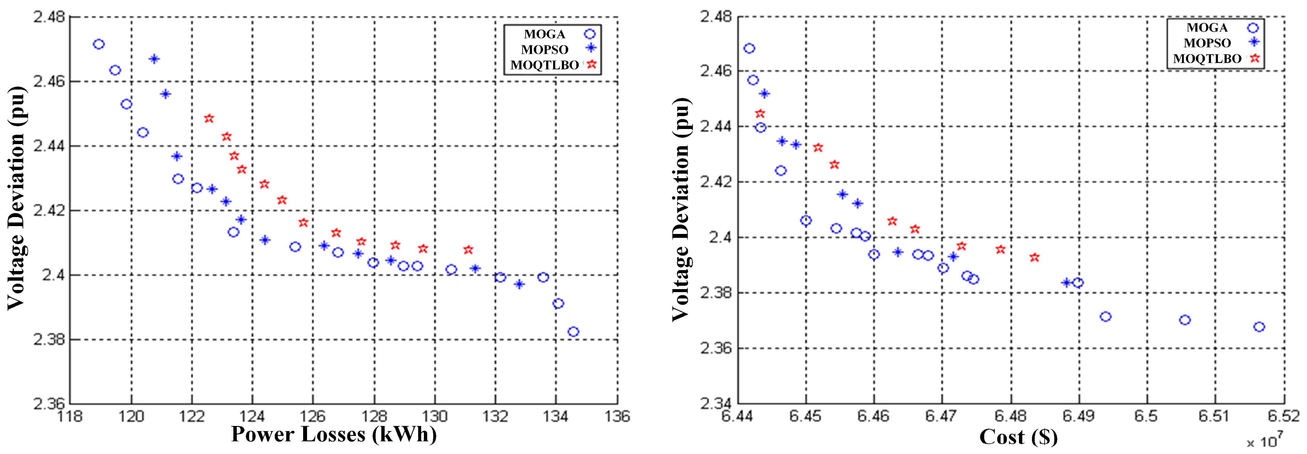
  • This paper compares the proposed algorithm’s optimal solutions and the best-reported optimization algorithms for DG placement in the distribution system to prove the superiority.
  • This paper compares the optimal solutions of DG placement in the cases of a similar type of DG for fuel cells, photovoltaic units, wind turbines, and a combination of all the mentioned DGs.
  • This paper presents a methodology for integrating DG to improve the power quality issues of the distribution system.

2. Multi-Objective Formulation for Placement of Distributed Generators

In optimization problems, the multi-objective or single-objective approach can be employed to derive results based on the specified objective functions. Decision-makers play a crucial role in identifying their desired objective functions. The multi-objective approach is particularly relevant when conflicts arise among the objective functions. The main objective of this paper is to determine the optimal location and size of DG by effectively optimizing the proposed objective functions. This section presents the proposed objective functions and practical constraints that constitute the mathematical formulation of the problem.
Some efforts should be performed to point out the difficulties in finding and combining two optimization algorithms. First of all, the No Free Lunch Theorem shows that no algorithm is appropriate for all models. Therefore, suitable optimization algorithms should be selected for combination. In this regard, the literature review of the latest papers about DG placement helped this research to find TLBO and SA algorithms as the best ones in this specific optimization problem. The second difficulty is finding the advantages and disadvantages of each optimization algorithm to eliminate weaknesses. For example, the liability of these algorithms is that they go to local optimum solutions in some cases instead of optimum global ones. For this problem, this paper has used the nondominated solutions of both algorithms simultaneously to decrease the probability of achieving the unwanted local optimum solution. The last difficulty is finding the correct optimization technique to increase calculation velocity and accuracy. In this way, this paper has applied a fuzzy clustering technique.

2.1. Objective Functions

2.1.1. Total Electricity Generation Cost

In line with the economic considerations of DG, this paper formulates the cost function for each unit based on the specifications outlined in [39] and are as follows:
C p = ( C o s t 1 g e n + C o s t 2 g e n ) × p ,
C o s t 1 g e n = C a p × C o s t × A r L T × L F × 365 × 24
C o s t 2 g e n = F c o s t + O   &   M   c o s t
The total electricity generation cost mathematic model is as follows:
f 1 X = i = 1 N p v C p v P p v + j = 1 N f c C f c P f c + k = 1 N w i n d C w i n d ( P w i n d ) + c o s t s u b
c o s t s u b = Q s u b × P s u b
F 1 X = m i n [ f 1 X ]
The power and location vector of fuel cell units, photovoltaic units, and wind units represent X, which this paper will define in Section 3 by Equation (26). The optimization algorithm should minimize the first objective function, i.e., f 1 X [21].

2.1.2. The Bus Voltage Deviation

This paper defines the bus voltage deviation as follows:
f 2 X = m = 1 N b u s V n o m V r V n o m
F 2 X = m i n ( f 2 X )
The optimization algorithm should minimize the second objective function. i.e., f 2 X [23].

2.1.3. Power Losses

This paper determines the third objective function in the DG placement problem as follows [19,40]:
f 3 X = a = 1 N l t b = 1 N n b ( R m × I m 2 × t )
F 3 X = min ( f 3 X )

2.1.4. Emission

This paper calculates the total emission of greenhouse gases (i.e., E t ) such as nitrogen oxides (i.e., NOx) and Sulphur oxides (i.e., SOx) caused by fossil-fueled thermal units as follows:
E t = n = 1 n D G E n ( P n ) = n = 1 n D G ( α n P n 2 + β n P n + γ n + ξ n exp 9 λ n P n )
f 4 X = E t f c + E t w i n d + E t p v
F 4 X = m i n ( f 4 X )
The fourth objective function for minimizing by optimization algorithm is f 4 X [27].

2.2. Constraints

2.2.1. Limitation of Voltage

The permissible voltage limits are as follows:
V min V m V max

2.2.2. DG Unit’s Number

The distribution network losses may achieve near zero in the ideal case of supplying all loads with the local DG. But this assumption, in most cases, is infeasible because of the high capital investment cost for local installation. Consequently, this paper has recommended a limited DG number but minimizes loss as the objective function [9].
n D G N D G

2.2.3. Size of DG

This paper has calculated the DG size by considering DG maximum allowable investment [41] as follows:
n = 1 n D G K W D G n η P l o a d

2.2.4. Other Limitations

DG limitations: DG systems’ limitations for generating electricity are significant factors in solving DG placement in the distribution system. This paper assumed that photovoltaic units could only make constant power daily from 6:00 a.m. to 6:00 p.m., and wind turbines can generate continuous power all the time [42,43]. Wind turbines, photovoltaic units, and fuel cells are considered PQ models [1] of an ideal generator in a single time step. If future research requires additional restrictions, such as limitations on hydrogen storage for fuel cells or specific time intervals like a particular month or year or fluctuations of the photovoltaic units and wind turbines, these constraints should be explicitly formulated and integrated into the optimization problem in the part constraints.
Load flow limitations: The load flow limitation should be checked in each iteration of the optimization algorithm. This paper obtains all calculations of objective functions by using the backward–forward load flow results. In order to reduce the repetitive discussion, we refer the interested readers to [10], which has discussed the load flow equations in detail.
If future studies necessitate further limitations, such as incorporating demand response into constraints within the optimization problem definition or incorporating different types of generators or energy storage systems, the power generation elements should be added to the objective functions while their limitations to the constraints of the problem.

3. Proposed MOQTLBO Method

In this work, we introduce the MOQTLBO algorithm as a solution for DG placement and sizing. Initially, we present the modification to the TLBO algorithm to enhance computational efficiency and accuracy. Subsequently, we define the concepts of quasi-opposition-based learning and optimization within the context of this problem. Finally, we discuss the integration of these techniques to propose the MOQTLBO algorithm, which combines the benefits of the modified TLBO and quasi-opposition-based approaches for effective DG placement and sizing optimization.

3.1. Modification of the Original TLBO

This paper designs a new modification for TLBO, intending to improve the convergence accuracy and velocity. The combination of SA and TLBO algorithms expands the optimization algorithm’s population and prevents premature convergence to a local minimum [44]. The current study connects an SA algorithm to the TLBO algorithm for improving the TLBO algorithm. This paper discusses some of the used optimization techniques in Appendix A, which contains a Pareto concept for a multi-objective approach and the Best-compromise-Solution method. The original TLBO algorithm is summarized in Appendix B, making a better understanding of the proposed modification.
Initially, the population generation of the SA algorithm in each step is as follows [45]:
X k + 1 s a = 0.8 * X k o l d + r a n d * 1.2 * X k o l d 0.8 * X k o l d         X k + 1 s a = X k + 1 s a , 1 , X k + 1 s a , 2 , , X k + 1 s a , N
K represents the vector component number. The algorithm combines the SA vector with the target vector as follows:
X K n e w = X K S A                             i f   r a n d 1 > r a n d 2 X K v                                                                     o t h e r w i s e X K n e w = X K n e w , 1 , X K n e w , 2 , , X K n e w , N
This algorithm compares the trial vector ( X k n e w ) with target vector ( X k v ) in single-objective problems to find the capability of it becoming a succeeding population member as follows:
X K + 1 n e w = X K v             i f               f x ( X K v ) < f x ( X K n e w ) X K n e w                                                     o t h e r w i s e
This algorithm compares the trial vector ( X k n e w ) with target vector ( X k v ) in multi-objective problems as follows:
X K + 1 n e w = X K v             i f               f x X K v   d o m i n a t e   f x ( X K n e w ) X K n e w       i f                   f x ( X K n e w )   d o m i n a t e   f x X K v
The relation between the sign “<” in Equation (19) and “dominate” in Equation (20) is discussed in Appendix A by Equations (A1)–(A3). The algorithm uses the Max-Min method by applying the achieved μ x f X of Equation (A4) if none f x X K v and f x ( X K n e w ) dominate each other, as follows:
α 1 = min μ i 1 , μ i 2 , , μ i L , α 2 = min μ n e w 1 , μ n e w 2 , , μ n e w L , X k + 1 n e w = X k i             i f               α 1 > α 2 X k n e w               o t h e r w i s e

3.2. Quasi-Opposition-Based Learning

The current study combines the modified TLBO with quasi-opposition-based learning (QOBL), which leads to finding more feasible solutions in the closing of the global optimum solution. Initially, this paper presents the concept of QOBL and its application to speed up the modified TLBO convergence. This paper uses the QOBL idea in generation jumping and population initialization [34,46].
In applying QOBL, this paper uses the following definitions:
  • Opposite number
The opposite number is defined by:
z * = a + b z
where z ϵ [ a , b ] .
  • Quasi opposite number:
The definition of a quasi-opposite number is as follows:
z q o = r a n d ( c , z * )
where c = a + b 2 .
  • Quasi opposite point:
T Let Z = ( z 1 , z 2 , , z L ) be a point in L dimensional space, where z 1 , z 2 , , z L ϵ Y and z l ϵ a l , b l l ϵ 1,2 , , L . The opposite point Z * = ( z 1 * , z 2 * , , z L * ) is defined by:
z d * = a l + b l z l
  • Quasi opposite point:
The definition of a quasi-opposite point is as follows:
z d q o = r a n d ( C d , z d o )
where C d = a d + b d 2 , and z d a d , b d ; D = 1,2 , , d .

3.3. Quasi-Oppositional Based Optimization

The quasi-oppositional-based (QOB) optimization involves two sections: the QOB generation jumping and the QOB initialization. Table 1 shows the QOB initialization Pseudocode. Also, Table 1 displays the QOB generation jumping Pseudocode. The authors of [16] have presented a Pseudocode of the original TLBO Algorithm.

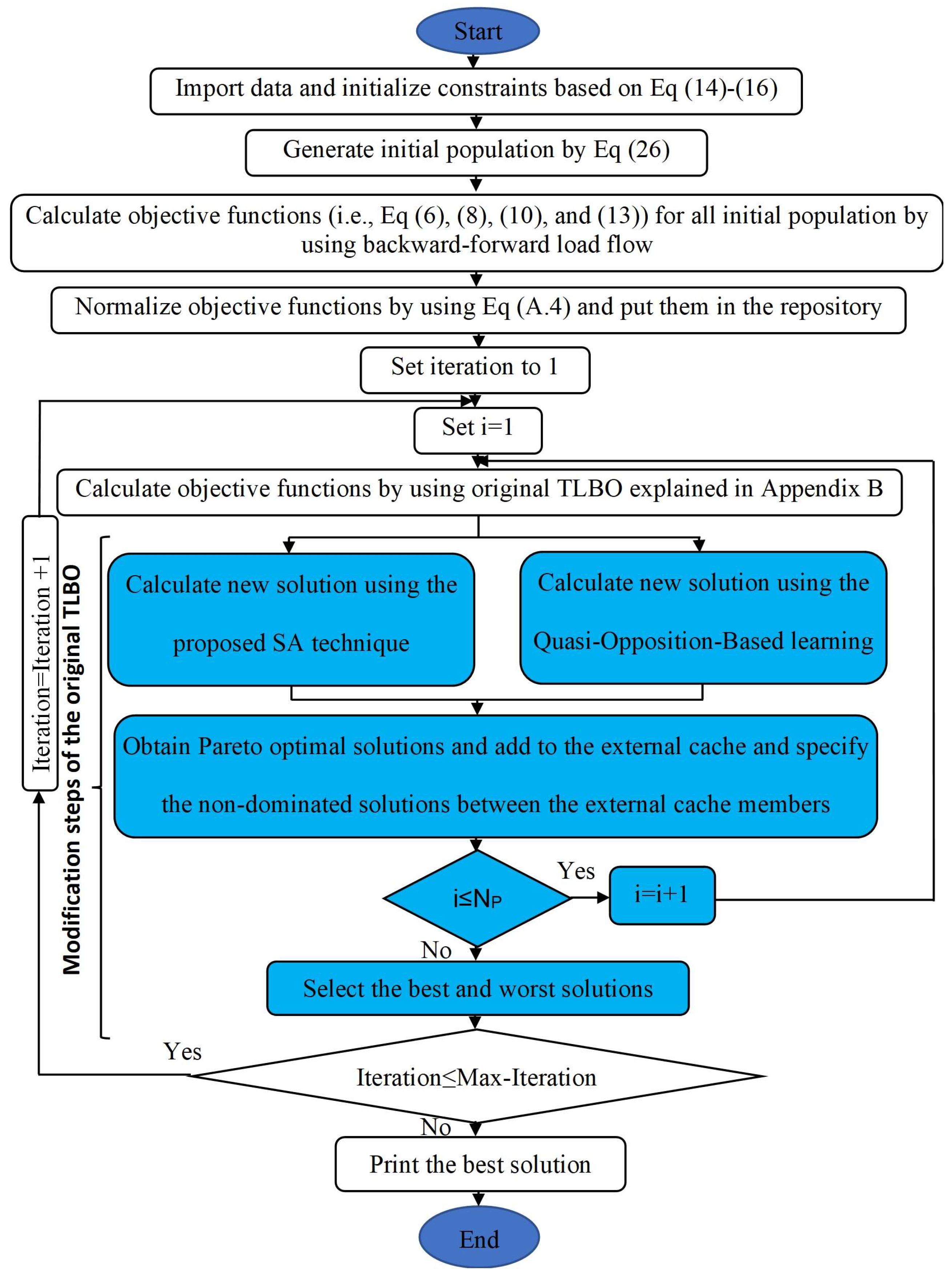
3.4. The Implementation of the Proposed MOQTLBO

The electric utilities (i.e., decision-makers of the optimization problem) first determined the objective functions based on the distribution system’s requirements, such as minimizing volt-age deviation and loss of the system. The permissible DG number using DG’s hosting capacity analysis of the distribution system is determined. The MQOTLBO algorithm can help the electric utility find the best place and size for the determined DG to optimize the objective functions. The MOQTLBO algorithm’s superiority is related to accuracy and calculation velocity to find the best optimum solutions. For applying the MOQTLBO algorithm in the DG placement problem, this paper takes the following steps into account, as Table 2 has shown, while Figure 1 shows the proposed algorithm’s flowchart.
As it is shown in Figure 1 and Table 2, the proposed algorithm includes two loops. The internal loop shows the individual updates from 1 to the number of population (np) to obtain their results. The external loop offers the iteration updates that result in collecting the best results among all iterations. In the case of weighted objective functions, the desired weight will be obtained in a way that i 4 w i = 1 . After calculating all non-dominated solutions by the proposed algorithm, the decision-maker can sort the obtained results by Equation (28), discussed in Section 5.2, as the selection of the best solution.
The definition of the initial population is as follows:
X r = L o c a t i o n 1 ,   , L o c a t i o n n ,   P 1 , P n ,   r = 1 , , n p ,   X = X 1 X 2 X n p n p F = F 11 F 21 F 31 F 41 F 12 F 22 F 32 F 42 F 1 n p F 2 n p F 3 n p F 4 n p
F 1 n p , F 2 n p , F 3 n p , and F 4 n p represent objective functions for the feasible solution number np. And also, n is the DG number, L o c a t i o n n is the nth DG location with the range between 1 and the maximum bus number, and the nth DG’s size with the range between 0 and the maximum size of the nth DG represented by P n . It is noteworthy that Xr has two variable types (i.e., discrete variables and continuous). These variables are related to the DG location (discrete) and the DG active power. This paper uses rounding function values for discrete variables.
The definition of the mean value in step 5 is as follows:
N = [ N 1 , N 2 , , N n ]

4. Conventional Optimization Approaches

As already mentioned in this work, the performance of the proposed method has been compared with that of conventional methods such as the GA, PSO, HBMO, and TLBO algorithms. Here, a brief description of each method is provided. GA is an evolutionary optimization technique inspired by the process of natural selection. It employs a population-based approach, where potential solutions evolve over generations through the application of genetic operators such as selection, crossover, and mutation. GA can explore a large search space, and its effectiveness lies in preserving promising solutions and gradually converging toward an optimal or near-optimal solution. More information on GA can be found in Refs. [37,46].
PSO is a population-based optimization algorithm that mimics the behavior of a social group. It operates by iteratively updating the positions and velocities of particles in a search space, with each particle influenced by its own best position and the best position found by the entire swarm. PSO emphasizes cooperation and information sharing among particles to search for the global optimum in the search space [9,22,26,27].
HBMO is a nature-inspired algorithm inspired by the mating behavior of honey bees. HBMO models the optimization problem as the process of finding the best mating partners among male and female bees. The algorithm iteratively improves the population through the stages of mating, recombination, and local search. HBMO utilizes the concept of neighborhood exploitation to enhance solution quality and convergence speed, making it suitable for various optimization problems. The algorithm, flowchart, Pseudo code, and all details of HBMO are available in [22,23].
TLBO is a metaheuristic algorithm inspired by the teaching and learning processes in a classroom. It employs a teacher and learner metaphor to optimize the objective function. In TLBO, the learner individuals improve their solutions by learning from the better solutions of the teacher individuals. This iterative process of teaching and learning aims to gradually improve the overall population and converge towards an optimal solution. Details of TLBO are available in Appendix B. Briefly, Table 3 displays the comparison of the mentioned optimization algorithms.

5. Simulation Results

This section shows the proposed optimization algorithm results for the DG placement problem. This paper presents the measured distribution system data in Appendix C. In essence, smaller systems lead to quicker solutions due to their simplicity, while larger systems demand more time due to their intricate nature. Smaller systems restrict ideal placements, whereas larger systems present abundant possibilities. The proposed algorithm efficiently manages large-scale challenges, offering speedy solutions, albeit without absolute certainty. In contrast, meticulous yet slower algorithms might yield superior results at the expense of time. Briefly, the choice of optimization algorithm should be tailored to the unique characteristics of the system at hand.
The proposed methods are implemented in the MATLAB software on a personal computer with an i7 core processor, 3.70 GHz, and 32 GB RAM. Two cases are analyzed, comparing the proposed algorithm with other evolutionary algorithms.
Case study 1 consists of two parts. Firstly, this paper considers single-objective optimization algorithms for the DG allocation. Thus, we suppose all four objective functions for solving the DG placement problem separately by running the single-objective optimization algorithms. The results of this part may be helpful for some decision-makers concerned with only one objective function.
Secondly, in case study 1, multi-objective optimization algorithms are considered using the Pareto optimal solution for DG placement in the distribution system. The results of two and three objective functions simultaneously optimized are presented in 2-dimensional and 3-dimensional spaces. Moreover, multi-objective optimization is applied, considering different weight options of the objective functions. Because of the variety in selection, nine cases are supposed to achieve the objective functions. This part may help decision-makers find the effectiveness of objective functions to each other and find the best solution in the specific projects.
In case study 2, this paper solves DG placement by a multi-objective optimization algorithm that considers different types of DG. In the first part, all the generators are the same in each simulation. The second part considers the combination of varying DG during the solving process. Case study 2 may help decision-makers to find the best renewable energy resources for specific projects.

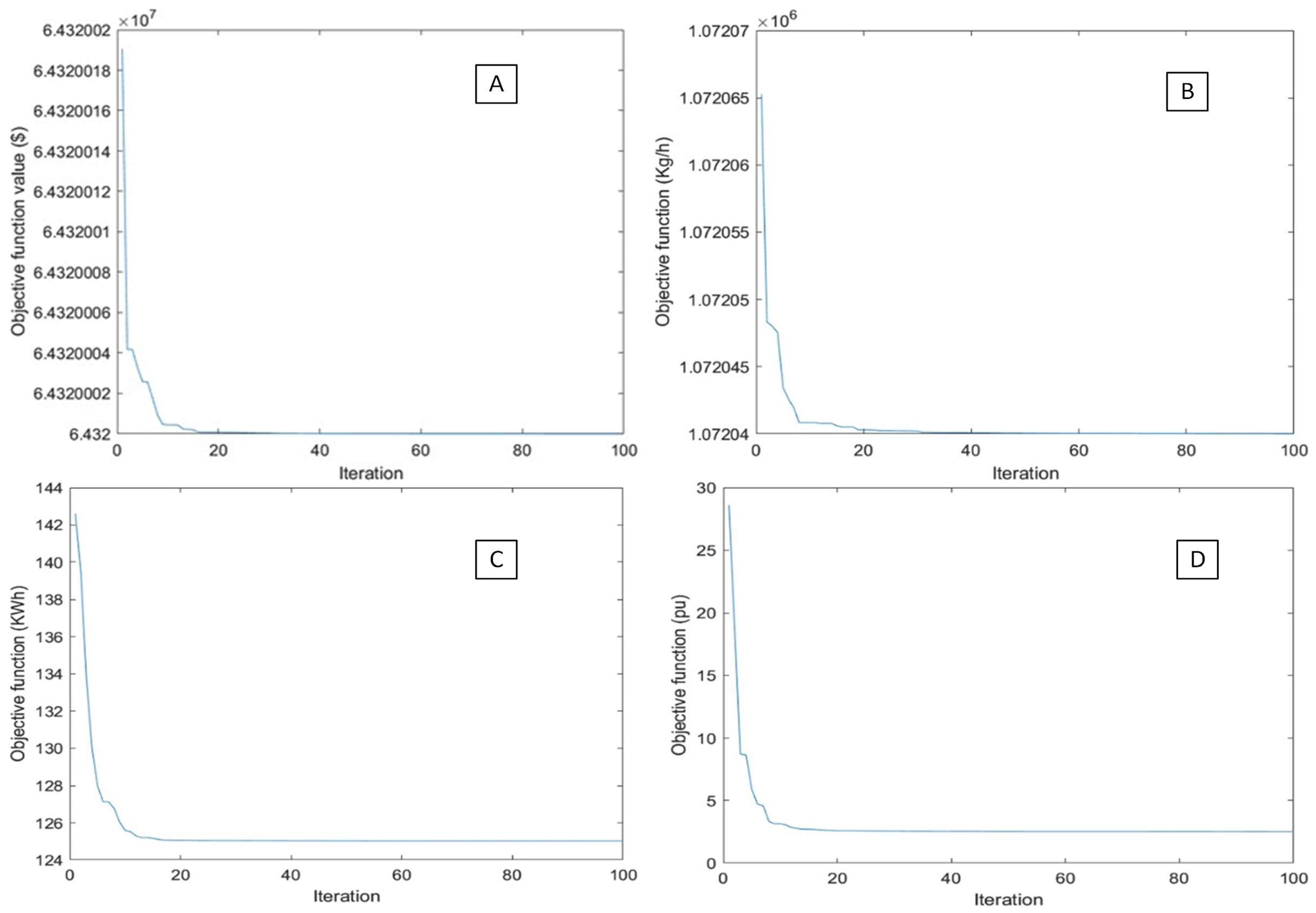
5.1. Case Study1: Part1—Single-Objective Results

Initially, to find the trade-off frontier’s extreme points, all four objective functions, namely the voltage deviation, total electrical losses, total emission, and total electrical energy cost, are optimized individually. In this regard, we should omit the Pareto concept mentioned in Section 3 (i.e., step 4). We have shown the results of PSO, GA, TLBO, HBMO, and MQOTLBO algorithms for all considered objective functions in Table 4. This paper selects the worst, average, and best results from feasible solutions after 50 trials of the simulation. This table displays the worst, best, and average results indicating the minimum, maximum, and intermediate obtained non-dominated solutions.
It is noteworthy that this paper has calculated the results of Table 4 in 50 trials. In the other analysis of this paper, we have considered 100 trials because obtained results in fewer trials (i.e., 50) are standard for comparing algorithms in the convergence velocity to the optimum solution. Also, the obtained results with more trials (i.e., 100) can be used to determine the superiority of the algorithms’ calculation accuracy. The proof of getting better outcomes for all objective functions is shown in Table 4.
This paper applies twelve fuel cells in this case. Their economic specification is the same as shown in Table 5, and their coefficients of emission are as follows: α = 4.285 K g h M W 2 , β = 5.094 K g h M W , γ = 4.586 K g h , ξ = 1.0 × 10 6 ,     a n d   λ = 8.00   M W 1 .
The location of DG, CPU time, and the best solutions obtained for the four objective functions are presented in separate tables (Table 6, Table 7, Table 8 and Table 9). The results presented in these tables demonstrate the superior performance of the MQOTLBO algorithm across multiple objective functions compared to other evolutionary algorithms. For instance, Table 6 illustrates that the MQOTLBO algorithm is approximately eight times faster than GA in achieving the best total cost solution. The calculation speed of these algorithms varies for different objective functions. For example, Table 7 demonstrates that the MQOTLBO algorithm is about four times faster than GA in finding the minimum voltage deviation solution, while Table 8 shows it is approximately 1.5 times faster in achieving the minimum loss function solution. Table 9 shows the results of different methods obtained by optimizing the emission and the MQOTLBO is the best one among them in calculation speed. It is worth emphasizing that all comparisons and evaluations were conducted on the same computer setup, ensuring a fair and unbiased assessment. The obtained results affirm the MQOTLBO algorithm’s potential as a promising optimization technique for DG location and related challenges in the field of power distribution systems.
We obtained the location of Fuel cell units by a single-objective MQOTLBO for different objective functions in the 70-bus test system, as shown in Figure 2.
This paper displays the convergence plot of MQOTLBO in Figure 3. This figure aims to show the capability of MQOTLBO to convergence. Parts A, B, C, and D of Figure 3 display the convergence of cost, emission, loss, and voltage deviation objective functions.
In this paper, the Friedman test among implemented optimization algorithms proves the superiority of the proposed algorithm. This paper uses the Friedman test to test for differences between results groups of optimization algorithms when measuring the dependent variable (i.e., objective function) is ordinal. Ref. [47] explains the formulation and coding of the Friedman test. The obtained Qs (i.e., test statistic) for the objective functions cost, loss, emission, and voltage deviations are 285.996, 276.348, 280.432, and 300, respectively, for 100 trials (i.e., n = 100), five algorithms (i.e., k = 5), and p-value (the level of significance) is considered less than 0.00001. The results are significant at p less than 0.10. A p-value, or probability value, is a number describing how likely it is that your data would have occurred by random chance. The level of statistical significance is often expressed as a p-value between 0 and 1. We refer the interested readers to [47] for finding the definition, meaning, and formulation of n, p, Q, and k. The Friedman test’s analysis shows that the best optimization algorithms for this specific optimization problem are MQOTLBO, TLBO, HBMO, PSO, and GA in order.

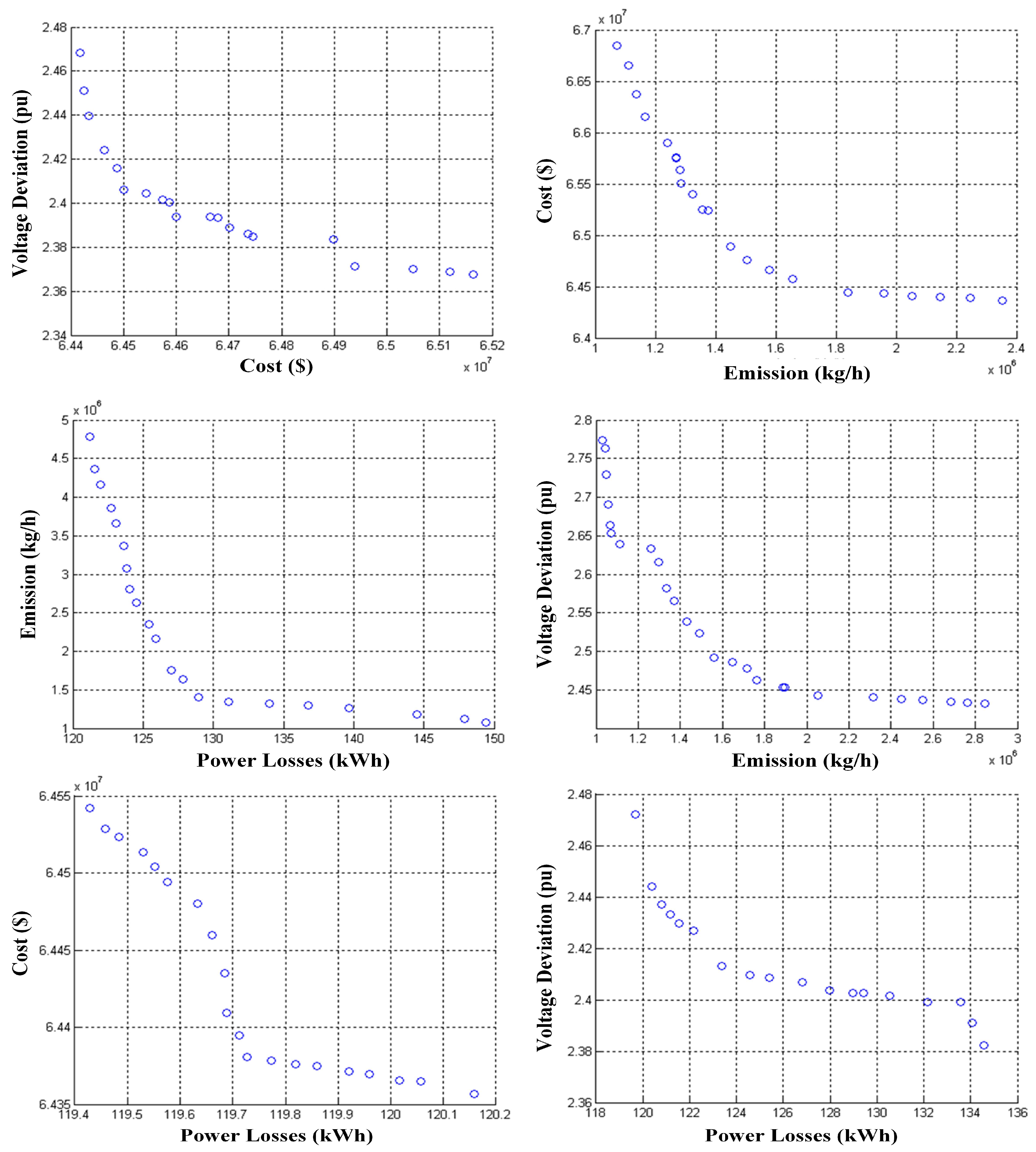
5.2. Case Study1: Part2—Multi-Objective Results

The concept of Pareto optimal solutions can help decision-makers select the best solution according to the comparing interests. We show the Pareto front obtained by MQOTLBO in Figure 4. Pareto optimal solutions are well distributed over the trade-off curves. Still, some objective functions, such as the cost and the power losses, offer some conflict with each other related to their formulations, as explained in Section 1.2.
This paper shows the obtained Pareto fronts by the MOPSO Algorithm [48], MOGA [49], and the proposed algorithm in Figure 5. Solutions of the proposed algorithm dominate the solutions obtained by MOPSO and MOGA. The proposed algorithm’s diversity is higher than other approaches because of the Quasi-opposition mechanisms used throughout the optimization process. We have shown only 2 out of 6 positions in Figure 5 for comparison.
Simultaneously optimizing three objective functions is shown in Figure 6 using three-dimensional diagrams. Different configurations are shown in Figure 6 to help the decision-maker (electric utility) choose the best solution.
To illustrate the improvement/worsening of each objective function to other ones, we have shown nine cases in Table 10. Cases I–IV involve single-objective optimization results, and the other issues are as follows:
  • Case V-assumed objectives: cost, power losses, and voltage deviation (i.e., f1, f2, and f3).
  • Case VI-assumed objectives: cost, voltage deviation, and emission (i.e., f1, f2, and f4).
  • Case VII-assumed objectives: power losses, voltage deviation, and emission (i.e., f2, f3, and f4).
  • Case VIII-assumed objectives: cost, power losses, and emission (i.e., f1, f3, and f4).
  • Case IX-assumed objectives: all objective functions (i.e., f1, f2, f3, and f4).
Selection of the best solution: In Table 10, cases I–IV show the results obtained by the single-objective of the proposed algorithm. In case I, the objective–function was total cost (f1), and we calculated the other objective–function values when f1 was at the minimum point. Moreover, Cases V–VIII show results obtained by optimizing three objective functions together.
Clearly, Figure 6 shows case VI of Table 10. Each Pareto optimal solution is an option assumed by the decision-maker.
The decision-maker of the distribution system (i.e., electricity utility) determines the weight factors for objective functions. In this determination, some issues are considered. First of all, the condition of the distribution system is the issue. For example, suppose the distribution system has a considerable amount of voltage deviation problem. In that case, the decision-maker to solve this problem selects a more significant weight factor voltage deviation compared to other objective functions because solving this problem is more important for this specific decision-maker. Secondly, the condition of the decision-maker or consumer is the issue. For example, suppose the decision-maker needs more benefits from selling electricity. In that case, the decision-maker determines a more significant weight factor for cost compared to other objective functions.
The system operator can adopt one of the optimal solutions for the particular frame based on its preferences over the objective functions. After obtaining all Pareto optimal solutions based on specific preferences, the decision-maker must select the best compromise solution. After applying the MQOTLBO to generate Pareto sets, the choice of the best-compromised solution performs as follows:
N μ l = i = 1 n w i × μ l i l = 1 m i = 1 n w i × μ l i
where m is the number of non-dominated solutions, n is the number of objective functions, and wi is the weight factor for the objective-function number k. It is noteworthy that the decision-maker should determine the importance of the objective function, such as Table 10, i.e., i 4 w i = 1 .
This paper proposed selecting best-compromise solutions among all Pareto optimal solutions, as shown in Table 10. The main points of the obtained results are as follows:
-
Comparing the obtained values of objective functions in Cases IV and IX-I shows that the voltage deviation value of Case IX-I (i.e., 1.4031) is lower than the voltage deviation of Case IV (i.e., 2.5059). Still, three other objective functions (i.e., cost, power loss, and emission) of Case IV are lower than Case IX–I. It means that the three objective functions’ worsened values in Case IV occur due to the reduction of voltage deviation in Case IX-I.
-
The first and second objective functions in case V have no conflict because when w1 and w2 are altered (decreased or increased), the objective functions do not change.
-
The objectives related to cost or power losses have the same behavior. The results of Cases I, II, III, IV, and V have proved this claim. In Cases I and III, cost and power losses have the same behavior. It means that when we minimize either cost or power loss individually, the other one is also minimized.
-
The cost and emission objective functions are conflicting with others. In Cases I, II, III, and IV, when the cost function is improved, the emission function is worsened and vice versa.

5.3. Case Study2: Part1—SAME Generators

This paper presents the effects of changing DG types in the second case study’s proposed optimization problem. We show results obtained by employing 10 kW and 100 kW wind turbines, photovoltaic units, and fuel cell units in Table 11. Their economic specification is the same as shown in Table 3. It is noteworthy that we considered that photovoltaic units and wind turbines can generate power continuously.
As shown in Table 11, when all 12 DG are fuel cell units, the cost function is the minimum value because of the lower capital cost of fuel cell units than the other used DG. On the other hand, the other used DG does not have emissions, while fuel cell units have. Some scholars have generally criticized intermittent generating power by renewable resources such as wind and solar power. Therefore, we should combine them with other continuous power generators. Using wind turbines or photovoltaic units as all power generators in this part is that obtained simulation results can help the decision-makers select a combination of renewable resources.

5.4. Case Study2: Part2—The Combination of Generators

This case study applies the combination of fuel cell units, photovoltaic units, and small wind turbines. In this regard, we assumed eight fuel cell units, two photovoltaic units, and two small wind turbines in this case study. The maximum generation of the small wind turbine, photovoltaic unit, and fuel cell unit are 10 kW, 100 kW, and 100 kW.
This paper assumed that small wind turbines could make power all the time and photovoltaic units could generate power only daily from 6:00 a.m. to 6:00 p.m. And also, other DG should compensate for the lack of power generation of photovoltaic companies.
This paper shows the current case study results in Table 12. We offer only ten positions of 104 calculated non-dominated solutions in Table 12. In this Table, we show the objective functions’ optimum values optimized separately in boldface. The current case study results show a slight increase in the cost-objective function, a decrease in the emission objective function, and a bit of change in the losses and voltage objective functions. The MQOTLBO algorithm obtains the results of this table.
The optimum values of objective functions, which are optimized separately, are shown in boldface.
The overall analysis of the results shows the superiority of the proposed method in calculation velocity and accuracy compared to the benchmark algorithms. These superiorities are because of the proposed modification that makes the parameters of the proposed algorithm needless to tuning during the optimization process and makes the population of non-dominated solutions more than before. Therefore, the proposed method could achieve the optimum solution more accurately and faster.
Generalizing that finding, everyone could expect that the proposed optimization algorithm may solve other optimization problems with single or multi-objectives. Additionally, the electric utility can use the proposed optimization algorithm to plan the installation of the future DG in the optimum location to improve power quality issues. For example, in Shiraz, a city located in Iran, the electric utility wants to install DG on the distribution system while considering the hosting capacity of the distribution system because of the interests of investors and customers to install DG as well as improving the voltage profile of the distribution system by using the integration of DG. In this case, the proposed optimization algorithm can help the electric utility find the best places and sizes of DG to allow the investors and customers to install DG.
Although this paper has proven the proposed method’s feasibility issues, some other support material from the practical perspective should be considered. The most important one is the complexity of the software to develop. Therefore, this paper suggests performing estimating software testing complexity [48] before implementing it practically. In addition, this method depends on personal factors such as relying on the print length, trust in the programmer’s style for writing source code, and how many statements one puts in one line. The estimating software testing complexity details are available in [50].
This paper’s results show that the proposed algorithm performs well in solving the DG placement problem. However, the No Free Lunch Theorem shows that no one algorithm is appropriate for all models. In this regard, the next step will be a sensitive and parameter analysis of the results to limit the proposed algorithm’s limitation in solving the optimization problems. Moreover, researchers can find the most valuable contributions in those that introduced nonlinear mathematical models and convexify them using some second-order cone programming (SOCP) and soft open point (SDP) relaxations for the 3-Ph unbalanced models.

6. Conclusions

A fast and accurate new hybrid multi-objective optimization algorithm (i.e., MQOTLBO) has been presented to handle complex, large-scale energy management problems, facilitate real-time decision-making, adapt to changing conditions, and optimize system performance. It is a Pareto-based optimization that leads to the best compromise solution by applying a fuzzy decision-making tool. The proposed algorithm has been employed for siting and sizing DG in the distribution network to optimize four objective functions.
Simulation results prove the proposed algorithm’s capability to minimize the cost of generation, losses, voltage deviations, and emission of greenhouse gasses in the test distribution system. The ability to obtain several Pareto optimal solutions to help the decision-maker select the best solution based on company preference and operating conditions of the policy are the main advantages of the proposed algorithm. The results obtained by other evolutionary algorithms such as PSO, GA, HBMO, and original TLBO compared with the suggested algorithm results proved the superiority of MQOTLBO in calculation speed and accuracy. For future planning of the distribution system, the electric utility can use the proposed optimization algorithm to benefit DG integration with the best size and location. In this regard, the electric utility should primarily consider the distribution system’s hosting capacity to install DG. They can then use the proposed optimization algorithm based on objective functions and determined DG.
In future research, integrating the proposed optimization algorithm with machine learning techniques can be explored to reduce human decision-making errors. Additionally, comparing the performance of the new optimization algorithms with the proposed method can lead to the discovery of more accurate and efficient optimization algorithms.

Author Contributions

Conceptualization, S.I.T.; methodology, S.I.T.; software, S.I.T.; validation, S.I.T., M.D. and M.H.A.; formal analysis, M.H.A.; investigation, M.H.A.; resources, S.I.T.; data curation, S.I.T.; writing—original draft preparation, S.I.T.; writing—review and editing, S.I.T., M.D., M.H.A.; visualization, M.D.; supervision, M.H.A.; project administration, M.H.A.; funding acquisition, M.H.A. All authors have read and agreed to the published version of the manuscript.

Funding

This research received no external funding.

Data Availability Statement

No new data were created.

Acknowledgments

The authors are pleased to acknowledge all support from the Dept. of Electrical and Computer Engineering at The University of Memphis, USA, to complete this work.

Conflicts of Interest

The authors declare no conflict of interest.

Abbreviations

A r Rate of annual interest
a , b Two real numbers ( b is bigger than a )
C a p The capacity of the generator [kW]
C f c Summation C o s t 1 g e n and C o s t 2 g e n when the generator is a fuel cell unit
C o s t Capital cost [$/kW]
C o s t 1 g e n The capital cost of the generator in the lifetime based on capacity, annual interest, and load factor
C o s t 2 g e n Summation of fuel cost and operation and maintenance cost
C p Cost function
C p v Summation C o s t 1 g e n and C o s t 2 g e n when a generator is a photovoltaic unit
c o s t s u b Cost of substation
C w i n d Summation C o s t 1 g e n and C o s t 2 g e n when the generator is a wind turbine
E n Emission of nth DG
E t The total emission of greenhouse gases from one kind of DG unit
E t f c The total emission of greenhouse gases from fuel cell units
E t p v The total emission of greenhouse gases from photovoltaic units
E t w i n d The total emission of greenhouse gases from wind turbines
f 1 X , f 2 X , f 3 X , f 4 X Total electricity generation cost, bus voltage deviation, power loss, and emission functions (objective functions)
F 1 X , F 2 X , F 3 X , F 4 X Minimized total electricity generation cost, bus voltage deviation, power loss, and emission functions
F c o s t Fuel cost [$/kWh]
f p   ( X ) , f q X pth and qth objective functions
f x max , f x min Upper and lower limits of f x ( X )
f x ( X ) The xth objective function
H A constant between 0 and 1
I m Actual current mth branch of the distribution system
j r r Jumping rate
K W D G n The capacity of the nth DG
L Number of objective functions in multi-objective problems
L F Load factor
L T Lifetime [year]
α Any value for which the normal distribution function is required
α 1 Minimum of membership function of ith feasible solution
α 2 Minimum of membership function of the new feasible solution
α n , β n , γ n , γ n , ξ n Emission characteristics coefficient of nth DG
t Time step [year]
μ Membership function
N b u s Maximum number of buses
N f c Number of fuel cell units
N l t The lifetime of DG units
N n b Number of distribution system branches
N p v Number of photovoltaic units
N w i n d Number of wind units
O & M c o s t Operation and maintenance cost of DG units
p Active power [kW]
P f c The power generated by the fuel cell unit
P l o a d Total load power
P n The electrical output of the nth generator
P p v The power generated by the photovoltaic unit
P s u b Value of injected active power to the distribution system
P w i n d The power generated by the wind turbine
Q s u b Price of injected active power to the distribution system
R m Resistance mth branch of the distribution system
  v a r 2 Variance
V m The magnitude of the voltage at mth bus
V max , V min Upper and lower voltage limits
V n o m The nominal voltage of the mth bus of the distribution system
V r Voltage magnitude of the mth bus of the distribution system
X Vector of location and power for DG units
X n e w New learner (new member of the population)
X o l d Old learner (an old member of the population)
X r d i f f the contrast between the teacher’s learning Level and the mean of the class at any iteration
X r + 1 N e w New teacher’s learning level in iteration r + 1
X r O l d Teacher’s learning level in iteration r
X r Matrix of location (discrete numbers) and size (continuous numbers) of DG units
X x Learner x (feasible solution x)
X z Learner z (feasible solution z)
X K s a , v SA vector (with K vector component for vth member of population)
X K v Feasible solution vector (with K vector component for vth member of population)
X K n e w New generated members of the population
X K + 1 n e w Equal to X K n e w or X K v based on the mentioned conditions
Z Any real number between [a,b]
z * Opposite number
z d q o Quasi opposite point

Appendix A. Optimization Techniques

(a) Pareto concept for a multi-objective approach: The optimization algorithm may face a set of optimal trade-offs between the different objective functions. Therefore, in multi-objective optimization issues, the idea of optimality is supplanted with Pareto optimality [51,52]. A Pareto optimal solution is a solution that any other solution could not dominate. A vector of decision variables X * ϵ F is Pareto optimal if there does not exist another X ϵ F such that:
F = [ f 1 X f 2 X f o X ]
f p   ( X ) f p   ( X * )   f o r   a l l   p = 1,2 , , o  
f q X < f q X *   f o r   a t   l e a s t   o n e   q p
where o is the number of objective functions, and X is a feasible solution. In the minimization problem, solution X dominates the solution X * if both conditions of Equations (A2) and (A3).
(b) The Best compromise solution method: The decision-maker needs to select the best compromise solution among the Pareto sets after having the Pareto-optimal set of non-dominated results. Therefore, we suggest a fuzzy concept to normalize the objective functions. A membership function represents the ith objective function ( μ x f X ) define as [6]:
μ x f X = f x max f x ( X ) f x max f x min               f o r             f x min f x ( X ) f x max 0                               f o r               f x ( X ) f x max 1                               f o r                 f x ( X ) f x min
The membership function comprises lower and upper restrictions, as shown in Figure A1. It is a strictly monotonically decreasing and continuous function [9]. The lower and upper limits (i.e., f x min and f x max ) of each objective function are established to produce a membership function μ x f X for each objective function (i.e., f x ( X ) ).
Figure A1. The illustration of membership functions for the objective function.
Computation 11 00214 g0a1

Appendix B. Original TLBO Algorithm

This algorithm is based on a teaching-learning concept aiming to increase the learner’s knowledge. The population members of this optimization algorithm are learners of a class. This algorithm obtains the global solutions without any specific control parameters by generating generation numbers and population size [29]. To achieve the original TLBO algorithm’s primary function, assume two different classes with two dissimilar teachers (i.e., T 1 and T 2 ) and the same cleverness level learners.
We show the distribution of students’ scores in Figure A2a, in which M 1 and M 2 are the mean scores of class-1 and class-2. Class-2 has gained better results than class-1.
Figure A2. Learners score distribution (a) for classes 1 and 2 (b) for classes A and B.
Computation 11 00214 g0a2
This algorithm assumes that the best solution, fitness value, design variables, and optimization population are teachers, learners’ scores, different class subjects, and students’ groups. We have modeled the obtained students’ ratings of class-A with M A in Figure A2b. We select the best student as the teacher (i.e., T A in Figure A2b).
The teacher’s effort is to increase the class mean from M A to a new mean (i.e., M B in Figure A2b), which means improving learners’ knowledge. After this step, a new teacher with more excellent knowledge than the learners require for the class (i.e., T B in class-B, who is a knowledgeable population learner).
The learners’ score distribution is calculated as follows:
f α = 1 v a r 2 π e ( α m e a n ) 2 2 v a r 2
The algorithm has two learning modes: the teacher and learner phases.
Teacher phase: This phase is part of the algorithm related to the learners’ learning from the teacher. In this phase, the teacher attempts to increase the class’s mean result towards his/her insight level. We consider N r and I r as the class’s mean results and teacher of the iteration number r [51]. Also, we upgrade the solution by the contrast between the teacher’s insight level (i.e., I r ) and the mean result of the class (i.e., N r ) at any iteration that can be shown as follows:
X r d i f f = r a n d * ( I r R s * N r )
Rs represents the teaching factor for changing the class’s mean result. The R_s magnitude is either 1 or 2, which is obtained randomly with equal probability based on the suggestion of Ref. [32]. After conducting several experiments on many benchmark functions, the authors of Ref. [32] concluded that the algorithm performs better if the R_s value is selected as either 1 or 2. For the same reason, the r a n d is suggested to be considered a random number in the range ( 0,1 ).
We modify the existing solution as follows:
X r + 1 N e w = X r O l d + X r d i f f
Learner phase: This phase increases the learner’s knowledge through class interactions. Randomly, the learners cooperate during class activities [52].
We can design the mathematical model by choosing two students X x and X z , randomly where x z . We took the objective functions into account by X x and X z and compared them to solve the single-objective problem. X n e w can be obtained as follows:
X n e w = X o l d + r a n d * X x X z       f X x < f X z X n e w = X o l d + r a n d * X z X x                   o t h e r w i s e

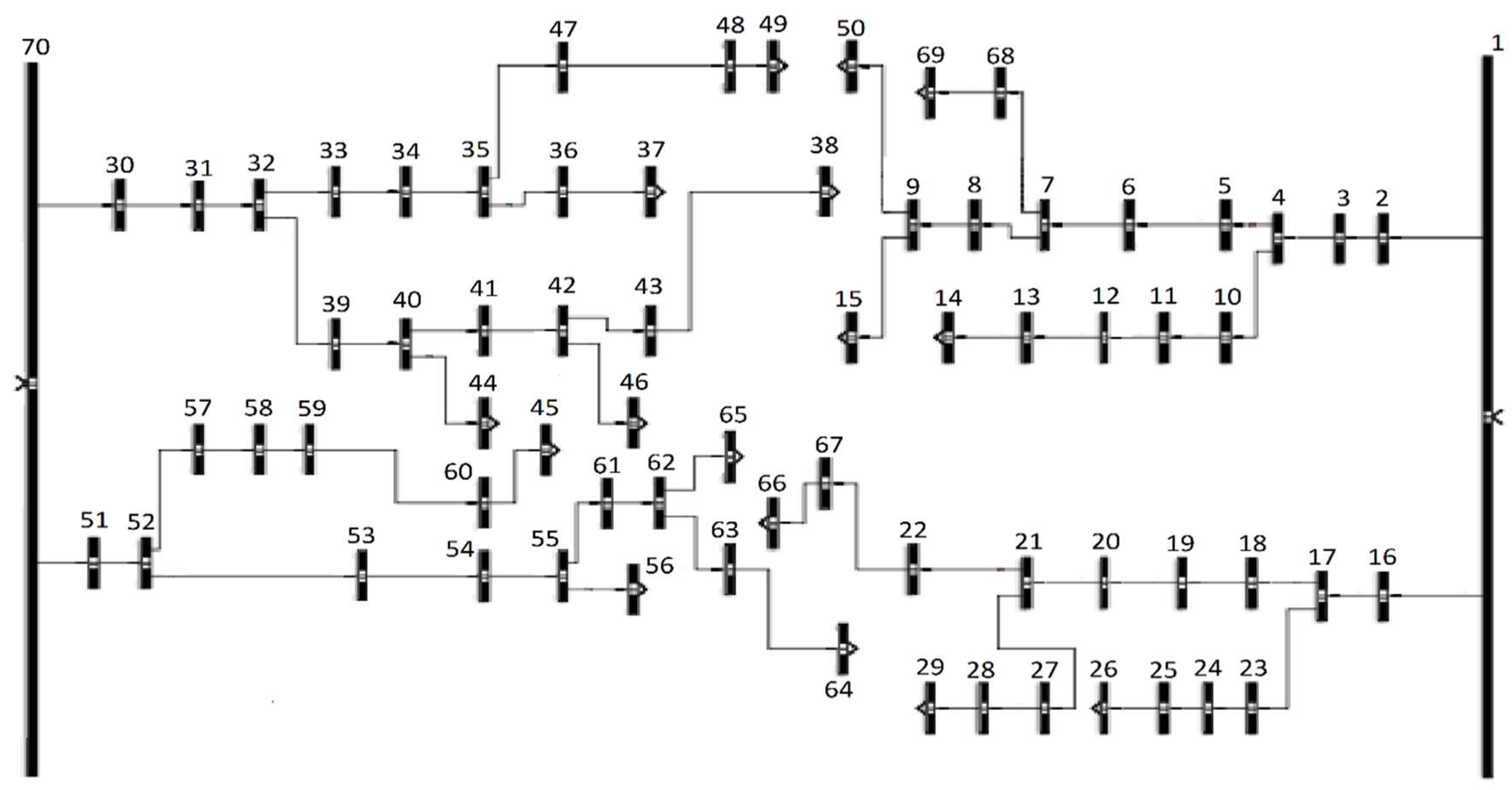
Appendix C. Test System Specification

This paper considers a standard test system that is shown in Figure A3. It is an 11-kV radial distribution system having 70 nodes, 69 branches, two substations, and four feeders [36]. The system data is shown in Table A1.
Figure A3. Test system.
Computation 11 00214 g0a3
Table A1. Test system Data.
Branch NumberSending BusReceiving BusR (Ω)X (Ω)p (kW)Q (kVAr)
1121.0971.074100.090.0
2231.4631.43260.040.0
3340.7310.716150.0130.0
4450.3660.35875.050.0
5561.8281.79015.09.0
6671.0971.07418.014.0
7780.7310.71613.010.0
8890.7310.71616.011.0
94101.0800.73420.010.0
1010111.6201.10116.09.0
1111121.0800.73450.040.0
1212131.3500.917105.090.0
1313140.8100.55025.015.0
1414151.9441.32140.025.0
157681.0800.734100.060.0
1668691.6201.10140.030.0
171161.0971.07460.030.0
1816170.3660.35840.025.0
1917181.4631.43215.09.0
2018190.9140.89513.07.0
2119200.8040.78730.020.0
2220211.1331.11090.050.0
2321220.4750.46550.030.0
2417232.2141.50560.040.0
2523241.6201.110100.080.0
2624251.0800.73480.065.0
2725260.5400.367100.060.0
2826270.5400.367100.055.0
2927281.0800.734120.070.0
3028291.0800.734105.070.0
3170300.3660.35880.050.0
3230310.7310.71660.040.0
3331320.7310.71613.08.0
3432330.8040.78716.09.0
3533341.1701.14550.030.0
3634350.7680.75240.028.0
3735360.7310.71660.040.0
3836371.0971.07440.030.0
3937381.4631.43230.025.0
4032391.0800.734150.0100.0
4139400.5400.36760.035.0
4240411.0800.734120.070.0
4341421.8361.24890.060.0
4442431.2960.88118.010.0
4540441.1880.80716.010.0
4644450.5400.367100.050.0
4742461.0800.73460.040.0
4835470.5400.36790.070.0
4947481.0800.73485.055.0
5048491.0800.734100.070.0
5149501.0800.734140.090.0
5270510.3660.35860.040.0
5351521.4631.43220.011.0
5452531.4631.43240.030.0
5553540.9140.89536.024.0
5654551.0971.07430.020.0
5755561.0971.07443.030.0
5852570.2700.18380.050.0
5957580.2700.183240.0120.0
6058590.8100.550125.0110.0
6159601.2960.88125.010.0
6255611.1880.80710.05.0
6361621.1880.807150.0130.0
6462630.8100.55050.030.0
6563641.6201.010130.020.0
6662651.0800.734130.0120.0
6765660.5400.367150.0130.0
6866671.0800.73425.015.0

References

  1. Taheri, S.I.; Salles, M.B.C.; Kagan, N. A New Modified TLBO Algorithm for Placement of AVRs in Distribution System. In Proceedings of the 2019 IEEE PES Conference on Innovative Smart Grid Technologies, ISGT Latin America 2019, Gramado, Brazil, 15–18 September 2019. [Google Scholar]
  2. Sabir, A.; Ibrir, S. A Robust Control Scheme for Grid-Connected Photovoltaic Converters with Low-Voltage Ride-through Ability without Phase-Locked Loop. ISA Trans. 2020, 96, 287–298. [Google Scholar] [CrossRef] [PubMed]
  3. Güler, N.; Irmak, E. Design, Implementation and Model Predictive Based Control of a Mode-Changeable DC/DC Converter for Hybrid Renewable Energy Systems. ISA Trans. 2021, 114, 485–498. [Google Scholar] [CrossRef] [PubMed]
  4. Sepehrzad, R.; Moridi, A.R.; Hassanzadeh, M.E.; Seifi, A.R. Intelligent Energy Management and Multi-Objective Power Distribution Control in Hybrid Micro-Grids Based on the Advanced Fuzzy-PSO Method. ISA Trans. 2021, 112, 199–213. [Google Scholar] [CrossRef] [PubMed]
  5. Gazijahani, F.S.; Ravadanegh, S.N.; Salehi, J. Stochastic Multi-Objective Model for Optimal Energy Exchange Optimization of Networked Microgrids with Presence of Renewable Generation under Risk-Based Strategies. ISA Trans. 2018, 73, 100–111. [Google Scholar] [CrossRef] [PubMed]
  6. Esmaeili, M.; Sedighizadeh, M.; Esmaili, M. Multi-Objective Optimal Reconfiguration and DG (Distributed Generation) Power Allocation in Distribution Networks Using Big Bang-Big Crunch Algorithm Considering Load Uncertainty. Energy 2016, 103, 86–99. [Google Scholar] [CrossRef]
  7. El-Fergany, A. Study Impact of Various Load Models on DG Placement and Sizing Using Backtracking Search Algorithm. Appl. Soft Comput. J. 2015, 30, 803–811. [Google Scholar] [CrossRef]
  8. Fu, G. An Explicit Divergence-Free DG Method for Incompressible Flow. Comput. Methods Appl. Mech. Eng. 2019, 345, 502–517. [Google Scholar] [CrossRef]
  9. Hadidian-Moghaddam, M.J.; Arabi-Nowdeh, S.; Bigdeli, M.; Azizian, D. A Multi-Objective Optimal Sizing and Siting of Distributed Generation Using Ant Lion Optimization Technique. Ain Shams Eng. J. 2018, 9, 2101–2109. [Google Scholar] [CrossRef]
  10. Das, B.; Mukherjee, V.; Das, D. Optimum DG Placement for Known Power Injection from Utility/Substation by a Novel Zero Bus Load Flow Approach. Energy 2019, 175, 228–249. [Google Scholar] [CrossRef]
  11. Niknam, T.; Taheri, S.I.; Mohammadi, M. Improvement and Revision of Polymer Electrolyte Membrane Fuel Cell Dynamic Model. Electr. Power Compon. Syst. 2010, 38, 1353–1369. [Google Scholar] [CrossRef]
  12. Ravindran, S.; Victoire, T.A.A. A Bio-Geography-Based Algorithm for Optimal Siting and Sizing of Distributed Generators with an Effective Power Factor Model. Comput. Electr. Eng. 2018, 72, 482–501. [Google Scholar] [CrossRef]
  13. Molver, I.; Chowdhury, S. Alternative Approaches for Analysing the Impact of Distributed Generation on Shunt Compensated Radial Medium Voltage Networks. Comput. Electr. Eng. 2020, 85, 106676. [Google Scholar] [CrossRef]
  14. Bayat, A.; Bagheri, A.; Noroozian, R. Optimal Siting and Sizing of Distributed Generation Accompanied by Reconfiguration of Distribution Networks for Maximum Loss Reduction by Using a New UVDA-Based Heuristic Method. Int. J. Electr. Power Energy Syst. 2016, 77, 360–371. [Google Scholar] [CrossRef]
  15. Iqbal, F.; Khan, M.T.; Siddiqui, A.S. Optimal Placement of DG and DSTATCOM for Loss Reduction and Voltage Profile Improvement. Alex. Eng. J. 2018, 57, 755–765. [Google Scholar] [CrossRef]
  16. Niknam, T.; Azizipanah-Abarghooee, R.; Aghaei, J. A New Modified Teaching-Learning Algorithm for Reserve Constrained Dynamic Economic Dispatch. IEEE Trans. Power Syst. 2013, 28, 749–763. [Google Scholar] [CrossRef]
  17. Kumar, S.; Mandal, K.K.; Chakraborty, N. Optimal DG Placement by Multi-Objective Opposition Based Chaotic Differential Evolution for Techno-Economic Analysis. Appl. Soft Comput. J. 2019, 78, 70–83. [Google Scholar] [CrossRef]
  18. ChithraDevi, S.A.; Lakshminarasimman, L.; Balamurugan, R. Stud Krill Herd Algorithm for Multiple DG Placement and Sizing in a Radial Distribution System. Eng. Sci. Technol. Int. J. 2017, 20, 748–759. [Google Scholar] [CrossRef]
  19. Kasaei, M.J.; Gandomkar, M.; Nikoukar, J. Optimal Management of Renewable Energy Sources by Virtual Power Plant. Renew. Energy 2017, 114, 1180–1188. [Google Scholar] [CrossRef]
  20. Bahmanifirouzi, B.; Niknam, T.; Taheri, S.I. A New Evolutionary Algorithm for Placement of Distributed Generation. In Proceedings of the 2011 IEEE Power Engineering and Automation Conference, Wuhan, China, 8–9 September 2011; Volume 1, pp. 104–107. [Google Scholar] [CrossRef]
  21. Niknam, T.; Taheri, S.I.; Aghaei, J.; Tabatabaei, S.; Nayeripour, M. A Modified Honey Bee Mating Optimization Algorithm for Multiobjective Placement of Renewable Energy Resources. Appl. Energy 2011, 88, 4817–4830. [Google Scholar] [CrossRef]
  22. Miao, D.; Hossain, S. Improved Gray Wolf Optimization Algorithm for Solving Placement and Sizing of Electrical Energy Storage System in Micro-Grids. ISA Trans. 2020, 102, 376–387. [Google Scholar] [CrossRef] [PubMed]
  23. Ayoubi, M.; Hooshmand, R.A. A New Fuzzy Optimal Allocation of Detuned Passive Filters Based on a Nonhomogeneous Cuckoo Search Algorithm Considering Resonance Constraint. ISA Trans. 2019, 89, 186–197. [Google Scholar] [CrossRef] [PubMed]
  24. Ramirez-Rosado, I.J.; Dominguez-Navarro, J.A. New Multiobjective Tabu Search Algorithm for Fuzzy Optimal Planning of Power Distribution Systems. IEEE Trans. Power Syst. 2006, 21, 224–233. [Google Scholar] [CrossRef]
  25. Khare, R.; Kumar, Y. A Novel Hybrid MOL-TLBO Optimized Techno-Economic-Socio Analysis of Renewable Energy Mix in Island Mode. Appl. Soft Comput. J. 2016, 43, 187–198. [Google Scholar] [CrossRef]
  26. Zou, F.; Chen, D.; Xu, Q. A Survey of Teaching–Learning-Based Optimization. Neurocomputing 2019, 335, 366–383. [Google Scholar] [CrossRef]
  27. Joshi, P.M.; Verma, H.K. An Improved TLBO Based Economic Dispatch of Power Generation through Distributed Energy Resources Considering Environmental Constraints. Sustain. Energy Grids Netw. 2019, 18, 100207. [Google Scholar] [CrossRef]
  28. Sahu, S.; Barisal, A.K.; Kaudi, A. Multi-Objective Optimal Power Flow with DG Placement Using TLBO and MIPSO: A Comparative Study. Energy Procedia 2017, 117, 236–243. [Google Scholar] [CrossRef]
  29. Elsisi, M.; Soliman, M. Optimal Design of Robust Resilient Automatic Voltage Regulators. ISA Trans. 2021, 108, 257–268. [Google Scholar] [CrossRef]
  30. Srikanth, M.V.; Yadaiah, N. An AHP Based Optimized Tuning of Modified Active Disturbance Rejection Control: An Application to Power System Load Frequency Control Problem. ISA Trans. 2018, 81, 286–305. [Google Scholar] [CrossRef]
  31. Biswas, P.P.; Mallipeddi, R.; Suganthan, P.N.; Amaratunga, G.A.J. A Multiobjective Approach for Optimal Placement and Sizing of Distributed Generators and Capacitors in Distribution Network. Appl. Soft Comput. J. 2017, 60, 268–280. [Google Scholar] [CrossRef]
  32. Mandal, B.; Roy, P.K. Optimal Reactive Power Dispatch Using Quasi-Oppositional Teaching Learning Based Optimization. Int. J. Electr. Power Energy Syst. 2013, 53, 123–134. [Google Scholar] [CrossRef]
  33. Taheri, S.I.; Vieira, G.G.T.T.; Salles, M.B.C.; Avila, S.L. A Trip-Ahead Strategy for Optimal Energy Dispatch in Ship Power Systems. Electr. Power Syst. Res. 2020, 192, 106917. [Google Scholar] [CrossRef]
  34. Zhang, J.; Li, Z.; Wang, B. Within-Day Rolling Optimal Scheduling Problem for Active Distribution Networks by Multi-Objective Evolutionary Algorithm Based on Decomposition Integrating with Thought of Simulated Annealing. Energy 2021, 223, 120027. [Google Scholar] [CrossRef]
  35. Taheri, S.I.; Salles, M.B.C.; Nassif, A.B. Distributed Energy Resource Placement Considering Hosting Capacity by Combining Teaching-Learning-Based and Honey-Bee-Mating Optimisation Algorithms. Appl. Soft Comput. 2021, 113, 107953. [Google Scholar] [CrossRef]
  36. Das, D. A Fuzzy Multiobjective Approach for Network Reconfiguration of Distribution Systems. IEEE Trans. Power Deliv. 2005, 21, 202–209. [Google Scholar] [CrossRef]
  37. Taheri, S.I.; Salles, M.B.C. A New Modification for TLBO Algorithm to Placement of Distributed Generation. In Proceedings of the 2019 International Conference on Clean Electrical Power (ICCEP), Otranto, Italy, 2–4 July 2019; IEEE: Piscataway, NJ, USA, 2019; pp. 593–598. [Google Scholar]
  38. Singh, B.; Mukherjee, V.; Tiwari, P. Genetic Algorithm Optimized Impact Assessment of Optimally Placed DGs and FACTS Controller with Different Load Models from Minimum Total Real Power Loss Viewpoint. Energy Build. 2016, 126, 194–219. [Google Scholar] [CrossRef]
  39. Das, B.; Mukherjee, V.; Das, D. DG Placement in Radial Distribution Network by Symbiotic Organisms Search Algorithm for Real Power Loss Minimization. Appl. Soft Comput. J. 2016, 49, 920–936. [Google Scholar] [CrossRef]
  40. Taheri, S.I.; Rodrigues, L.L.; Salles, M.B.; Sguarezi Filho, A.J. A Day-Ahead Hybrid Optimization Algorithm for Finding the Dispatch Schedule of VPP in a Distribution System. Simpósio Bras. Sist. Elétricos-SBSE 2020, 1, 1–6. [Google Scholar] [CrossRef]
  41. Taheri, S.I.; Salles, M.B.C.; Costa, E.C.M. Optimal Cost Management of Distributed Generation Units and Microgrids for Virtual Power Plant Scheduling. IEEE Access 2020, 8, 208449–208461. [Google Scholar] [CrossRef]
  42. Niknam, T.; Azizipanah-Abarghooee, R.; Rasoul Narimani, M. A New Multi Objective Optimization Approach Based on TLBO for Location of Automatic Voltage Regulators in Distribution Systems. Eng. Appl. Artif. Intell. 2012, 25, 1577–1588. [Google Scholar] [CrossRef]
  43. Hosseinpour, H.; Bastaee, B. Optimal Placement of On-Load Tap Changers in Distribution Networks Using SA-TLBO Method. Int. J. Electr. Power Energy Syst. 2015, 64, 1119–1128. [Google Scholar] [CrossRef]
  44. Sultana, S.; Roy, P.K. Multi-Objective Quasi-Oppositional Teaching Learning Based Optimization for Optimal Location of Distributed Generator in Radial Distribution Systems. Int. J. Electr. Power Energy Syst. 2014, 63, 534–545. [Google Scholar] [CrossRef]
  45. Frey, B.B. Friedman Test. In The SAGE Encyclopedia of Educational Research, Measurement, and Evaluation; SAGE: Sauzend Oaks, CA, USA, 2018. [Google Scholar]
  46. Rathore, A.; Patidar, N.P. Optimal Sizing and Allocation of Renewable Based Distribution Generation with Gravity Energy Storage Considering Stochastic Nature Using Particle Swarm Optimization in Radial Distribution Network. J. Energy Storage 2021, 35, 102282. [Google Scholar] [CrossRef]
  47. Hemeida, A.M.; Bakry, O.M.; Mohamed, A.-A.A.; Mahmoud, E.A. Genetic Algorithms and Satin Bowerbird Optimization for Optimal Allocation of Distributed Generators in Radial System. Appl. Soft Comput. 2021, 111, 107727. [Google Scholar] [CrossRef]
  48. Ferrer, J.; Chicano, F.; Alba, E. Estimating Software Testing Complexity. Inf. Softw. Technol. 2013, 55, 2125–2139. [Google Scholar] [CrossRef]
  49. Kianmehr, E.; Nikkhah, S.; Rabiee, A. Multi-Objective Stochastic Model for Joint Optimal Allocation of DG Units and Network Reconfiguration from DG Owner’s and DisCo’s Perspectives. Renew. Energy 2019, 132, 471–485. [Google Scholar] [CrossRef]
  50. Alva, S.; Manjunath, V. Strategy-Proof Pareto-Improvement. J. Econ. Theory 2019, 181, 121–142. [Google Scholar] [CrossRef]
  51. Rao, R.V.; Savsani, V.J.; Vakharia, D.P. Teaching-Learning-Based Optimization: A Novel Method for Constrained Mechanical Design Optimization Problems. Comput. Aided Des. 2011, 43, 303–315. [Google Scholar] [CrossRef]
  52. Venkata Rao, R. Review of Applications of Tlbo Algorithm and a Tutorial for Beginners to Solve the Unconstrained and Constrained Optimization Problems. Decis. Sci. Lett. 2016, 5, 1–30. [Google Scholar] [CrossRef]
Figure 1. Flowchart of the proposed optimization algorithm.
Computation 11 00214 g001
Figure 2. Location of 12 Fuel cell units with different objective functions by the single-objective MQOTLBO algorithm in the 70-bus distribution system.
Computation 11 00214 g002
Figure 3. MQOTLBO convergence curves for (A) the cost, (B) emission, (C) losses, and (D) voltage deviation.
Computation 11 00214 g003
Figure 4. Pareto front obtained using the MQTLBO algorithm.
Computation 11 00214 g004
Figure 5. Comparison of various methods by their obtained Pareto fronts.
Computation 11 00214 g005
Figure 6. Pareto front of three objective functions.
Computation 11 00214 g006
Table 1. Pseudocodes of quasi-oppositional based initialization and quasi-oppositional based generation jumping.
MethodPseudocode
Quasi-oppositional based initializationBegin
      For d = 1: n p ( n p = population size)
         For l = 1: n d ( n d = controlvariable)
              x d l q 0 = r a n d ( a l + b l 2 , a l + b l x d l )
         End
      End
End
Quasi-oppositional based generation jumpingBegin
      If rand (0,1) < j r r
          For d = 1: n p
             For l = 1: n d
                x d l q 0 = r a n d ( a l + b l 2 , a l + b l x d l )
             End
          End
      End
End
Table 2. MOQTLBO algorithm to approach DG placement.
StepsDescription
Step 1The first step defines the algorithm’s inputs, such as population size, the iterations number, DG numbers, DG characteristics, constraints, and network data.
Step 2This step calculates the initial population by using Equation (26).
Step 3The third step firstly calculates the objective functions vectors (i.e., Equations (6), (8), (10) and (13)) by using the backward-forward distribution load flow [10] (this paper obtains all calculations of objective functions by using the results of backward-forward load flow). Secondly, this step normalizes them by Equation (A4).
Step 4This step calculates Pareto optimal solutions by normalized objective function vectors of Step 3, and it saves them in the external cache.
Step 5This step computes the population mean column-wise, such as in Equation (27). The algorithm randomly selects a Pareto optimal solution of the external cache as a teacher ( X o l d ). Then, it calculates Xnew according to Equation (A7) using Xdiffk obtained from Equation (A6).
Step 6This step is the Learner phase. The algorithm checks the limitations of the considered elements. If an independent variable is higher than the maximum level, the algorithm makes it similar to the top level. If it is less than the minimum level, the algorithm changes identically to the minimum value. This step calculates the new vector’s objective functions (i.e., X n e w ) and compares them with the existing vectors in the external cache. The algorithm approves it ( X n e w ) by Equation (19) or Equation (20).
Step 7This step obtains a new population member (SA vector) by Equation (17) and then calculates Xk+1new y Equation (20) and, after that, compares it with the existing vectors in the external cache. Finally, this step adds Pareto optimal solutions to the external cache.
Step 8This step is Quasi-opposition-based learning modification. This step generates the QOP set and calculates the corresponding fitness values.
Step 9This step chooses the required fittest vector number from Xi and QOP as a new population set.
Step 10Firstly, this step classifies the solutions to find the best one. Secondly, it assigns that solution to the new teacher. Thirdly, this step modifies each student’s grade based on the new teacher’s knowledge (i.e., modifying Xi). Lastly, the algorithm obtains Pareto optimal solutions and adds them to the external cache.
Step 11This step specifies the non-dominated solutions of the external cache. The algorithm added some solutions in steps 7 and 10, and they might dominate existing solutions. Consequently, the algorithm needs to apply the Pareto method to find the non-dominated answers among the old and new external cache members.
Step 12This step makes a loop by going back to Step 5 until the present iteration number equals the maxi-mum iteration number.
Table 3. Conventional optimization algorithm comparison.
AlgorithmPrincipleStrengthsWeaknesses
GABased on the process of natural selection, involving selection, crossover, and mutation operations on a population of potential solutions.Effective for exploring large solution spaces, suitable for complex, multimodal, and nonlinear optimization problems.Can get stuck in local optima, requires tuning of parameters, and may have slow convergence rates for some problems.
PSOMimics the social behavior of birds flocking, where particles adjust their positions based on their own best experience and the swarm’s collective knowledge.Fast convergence, easy implementation, and good at escaping local optima. Suitable for continuous and discrete optimization problems.Convergence to global optimum is not always guaranteed; performance highly depends on parameters and initialization.
HBMOInspired by the mating behavior of honey bees.Suitable for both continuous and discrete problems, capable of escaping local optima, and often effective for complex, multimodal functions.Requires careful parameter tuning, might have longer convergence times for some problems, and could be sensitive to initializations.
TLBOSimulates the teaching and learning processes in a classroom, where learners (solutions) improve over iterations by learning from each other and a teacher (best solution).Simplicity in implementation, less parameter tuning, and robust performance for various problem types. It’s particularly effective in continuous optimization.Can be sensitive to the initial population, might struggle with discrete or combinatorial problems, and might require more iterations for convergence in certain cases.
Table 4. Worst, best, and average results after 50 trials (cost ( f 1 ), voltage deviation ( f 2 ), loss ( f 2 ), emission ( f 4 )).
ObjectiveAlgorithmAverageBest ResultWorst Result
f 1 ( $ ) GA [46]6.531 × 1076.512 × 1076.568 × 107
PSO [45]6.526 × 1076.501 × 1076.555 × 107
HBMO [35]6.517 × 1076.499 × 1076.540 × 107
TLBO [35]6.493 × 1076.474 × 1076.511 × 107
MQOTLBO6.453 × 1076.433 × 1076.502 × 107
f 2 ( p u ) GA [46]2.558472.563842.58964
PSO [45]2.562172.555542.57894
HBMO [35]2.557842.541942.56985
TLBO [35]2.527192.515152.54573
MQOTLBO2.511022.505982.53169
f 3 ( k W h ) GA [46]132.7814129.5982135.8975
PSO [45]130.1585128.9817132.2548
HBMO [35]128.4562128.0254129.8372
TLBO [35]127.0255126.2418128.2651
MQOTLBO126.0288125.0252127.2222
f 4 ( k g / h ) GA [46]1.22908 × 1061.21003 × 1061.25609 × 106
PSO [45]1.08601 × 1061.08002 × 1061.08928 × 106
HBMO [35]1.08250 × 1061.07382 × 1061.08530 × 106
TLBO [35]1.07601 × 1061.07225 × 1061.07912 × 106
MQOTLBO1.07559 × 1061.07204 × 1061.07906 × 106
Table 5. Economic specification of the implemented DG.
DG TypeFuel CellPhotovoltaic UnitsWind Turbine (Small)Wind Turbine (Big)
Rated capacity (kW)10010010100
Capital cost ($/kW)3674667538661500
Fuel cost ($/kWh)0.029000
Operation and Maintenance cost ($/kWh)0.010.0050.0050.005
Lifetime (year)10202020
Table 6. Results of different methods obtained by optimizing the cost function.
MethodCost ($)DG Placement (Bus Number)CPU Time (s)
GA [46]6.508 × 1071, 2, 3, 13, 21, 29, 31, 33, 34, 44, 52, 53572.63
PSO [45]6.480 × 1071, 2, 3, 14, 21, 29, 31, 33, 34, 44, 52, 53354.2
HBMO [35]6.489 × 1071, 2, 3, 14, 21, 29, 31, 33, 34, 44, 52, 53102.3
TLBO6.471 × 1071, 2, 3, 14, 21, 29, 31, 33, 34, 44, 52, 5375.26
MQOTLBO6.432 × 1071, 2, 3, 14, 21, 29, 31, 33, 34, 44, 52, 5370.32
Table 7. Results of different methods obtained by optimizing voltage deviation of buses.
MethodVoltage Deviation (pu)DG Placement (Bus Number)CPU Time (s)
GA [46]2.5478710, 12, 13, 18, 28, 34, 35, 44, 51, 53, 66, 67445.12
PSO [45]2.5258811, 12, 13, 18, 28, 34, 35, 44, 51, 53, 66, 67226.18
HBMO [35]2.5232511, 12, 13, 18, 28, 34, 35, 44, 51, 53, 66, 67124.1
TLBO2.5125511, 12, 13, 18, 28, 34, 35, 44, 51, 53, 66, 67115.67
MQOTLBO2.5059811, 12, 13, 18, 28, 34, 35, 44, 51, 53, 66, 67110.52
Table 8. Results of different methods obtained by optimizing the total power losses.
MethodPower Losses (KWh)DG Placement (Bus Number)CPU Time (s)
GA [46]128.32586, 7, 8, 23, 30, 31, 41, 44, 58, 59, 66, 67147.21
PSO [45]127.15747, 8, 9, 23, 30, 31, 41, 44, 58, 59, 66, 69306.81
HBMO [35]126.23126, 8, 9, 23, 30, 31, 41, 44, 58, 59, 66, 67123.89
TLBO126.22586, 8, 9, 23, 30, 31, 41, 44, 58, 59, 66, 67110.56
MQOTLBO125.01846, 8, 9, 23, 30, 31, 41, 44, 58, 59, 66, 67104.74
Table 9. Results of different methods obtained by optimizing the emission.
MethodEmission (Kg/h)DG Placement (Bus Number)CPU Time (s)
GA [46] 1.15122 × 10 6 6, 7, 8, 23, 30, 31, 41, 44, 58, 59, 66, 67444.46
PSO [45] 1.07550 × 10 6 7, 9, 10, 23, 30, 31, 41, 44, 58, 59, 66, 67252.49
HBMO [36] 1.07241 × 10 6 7, 9, 10, 23, 30, 31, 41, 44, 58, 59, 66, 67122.78
TLBO 1.07225 × 10 6 7, 9, 10, 23, 30, 31, 41, 44, 58, 59, 66, 67115.52
MQOTLBO 1.07204 × 10 6 7, 9, 10, 23, 30, 31, 41, 44, 58, 59, 66, 67110.29
Table 10. Single-objective and multi-objective results of MQOTLBO in cases with different weights.
CasesImportanceCost
($)
Power Losses
(KWh)
Voltage Deviation
(PU)
Emission
(Kgr/h)
W1W2W3W4
Case I----6.432 × 107125.69822.52891.07903 × 106
Case II----6.501 × 107127.49352.58011.07204 × 106
Case III----6.433 × 107125.01842.52571.07542 × 106
Case IV----6.457 × 107126.80102.50591.07447 × 106
Case V0.330.330.33-6.4660 × 107128.89382.3800-
0.20.40.4-6.4443 × 107125.54600.1775-
0.40.20.4-6.4443 × 107125.54600.3732-
0.40.40.2-6.4443 × 107125.54600.3732-
Case VI0.33-0.330.336.4820 × 107-2.50981.5100 × 106
0.2-0.40.46.4725 × 107-0.36911.0772 × 106
0.4-0.20.46.4725 × 107-0.36911.0752 × 106
0.4-0.40.26.4725 × 107-0.17461.0762 × 106
Case VII-0.330.330.33-135.93350.30241.0785 × 106
-0.20.40.4-135.93350.38081.0785 × 106
-0.40.20.4-135.93350.37081.0785 × 106
-0.40.40.2-133.59850.15611.0808 × 106
Case VIII0.330.33-0.337.6062 × 107150.4555-1.0757 × 10⁶
0.20.4-0.46.8058 × 107148.2527-1.0807 × 10⁶
0.40.2-0.46.8059 × 107126.2527-1.0807 × 10⁶
0.40.4-0.26.8057 × 107130.0764-1.0807 × 10⁶
Case IX0.250.250.250.257.6813 × 107141.93351.40311.2657 × 106
0.10.30.30.37.7172 × 107139.21451.30511.1659 × 106
0.30.10.30.37.6063 × 107140.78651.27471.2554 × 106
0.30.30.10.37.5772 × 107138.83211.70141.2453 × 106
0.30.30.30.17.6270 × 107133.34720.39091.2873 × 106
Table 11. Comparison of using different types of DG.
DG TypeCost ($)Voltage Deviation (pu)Power Losses (kWh)Emission (kg/h)
10 kW Wind Turbine6.884 × 1072.88549791.19020
100 kW Wind Turbine300.361 × 1072.124123144.98120
Photovoltaic12.919 × 1072.169854121.68120
Fuel cell with CHP6.437 × 1072.3854111.15621.07305 × 106
Table 12. Results for all objective functions and DG placement in the proposed system.
Cost ($)Voltage Deviation (per unit)Power Losses (kWh)Emission (ton/h)Location of Fuel Cell UnitsLocation of Photovoltaic UnitsLocation of Wind Units
8.426 × 1072.569853134.68571.024 × 1064,7,12,14,21,29,31,3322,6956,57
8.487 × 1072.552981135.74121.072 × 1065,11,22,34,35,44,47,4915,6656,60
8.506 × 1072.694219119.55991.065 × 1066,8,18,23,31,33,39,4866,695,26
8.518 × 1072.727727116.99981.03 × 1069,23,30,31,41,44,58,5922,4557,60
8.525 × 1072.457199126.79231.069 × 10611,18,40,47,50,59,62,6445,6632,35
8.510 × 1072.777587127.12481.066 × 10611,19,40,44,56,57,60,6415,4554,60
8.522 × 1072.565555128.74981.014 × 10611,17,43,44,52,57,62,6415,225,60
8.527 × 1072.647498129.74591.061 × 1068,9,11,13,50,59,65,6922,4560,64
8.533 × 1072.384455135.12891.051 × 1064,8,11,22,41,46,58,6645,6932,57
8.542 × 1072.484489129.33551.075 × 1067,12,25,33,44,52,67,6922,6654,56
Disclaimer/Publisher’s Note: The statements, opinions and data contained in all publications are solely those of the individual author(s) and contributor(s) and not of MDPI and/or the editor(s). MDPI and/or the editor(s) disclaim responsibility for any injury to people or property resulting from any ideas, methods, instructions or products referred to in the content.

