Article

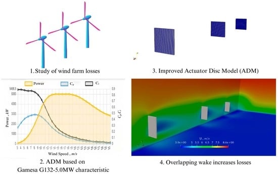
Modeling of Wind Turbine Interactions and Wind Farm Losses Using the Velocity-Dependent Actuator Disc Model

Department of Cryogenics and Aerospace Engineering, Wroclaw University of Science and Technology, Wybrzeże Wyspiańskiego 27, 50-370 Wroclaw, Poland
*
Author to whom correspondence should be addressed.
Computation 2023, 11(11), 213; https://doi.org/10.3390/computation11110213
Submission received: 20 September 2023 / Revised: 25 October 2023 / Accepted: 26 October 2023 / Published: 1 November 2023
(This article belongs to the Special Issue 10th Anniversary of Computation—Computational Engineering)

Abstract

:
This paper analyzes the interaction of wind turbines and losses in wind farms using computational fluid dynamics (CFD). The mathematical model used consisted of three-dimensional Reynolds-averaged Navier–Stokes (RANS) equations, while the presence of wind turbines in the flow was simulated as additional source terms. The novelty of the research is the definition of the source term as a velocity-dependent actuator disc model (ADM). This allowed for modeling the operation of a wind farm consisting of real wind turbines, characterized by power coefficients C p and thrust force coefficients C T , which are a function of atmospheric wind speed. The calculations presented used a real 5 MW Gamesa turbine. Two different turbine spacings, 5D and 10D, where D is the diameter of the turbine, and two different locations corresponding to the offshore and onshore conditions were examined. The proposed model can be used to analyze wind farm losses not only in terms of the geometric distribution of individual turbines but also in terms of a specific type of wind turbine and in the entire wind speed spectrum.

Graphical Abstract

1. Introduction

The use of wind energy has increased significantly since 2000, reaching 906 GW of installed capacity in 2022 [1]. Consequently, wind energy electricity production has increased substantially and was responsible for approximately 7.5% of global electricity production in 2022 [2]. According to IRENA data, global wind power generation capacity, including both offshore and onshore installations, has experienced a remarkable growth of almost 98 times over the past two decades [3]. In the case of onshore wind turbines the increase was from 22 GW in 2001 to 842 GW in 2022. In comparison, the offshore wind capacity has grown from zero in 2002 to 64 GW in 2022 [1]. Most newly installed wind turbines are three-blade units with a horizontal axis of rotation, characterized by the highest efficiency exceeding 50 % [4]. In the coming years, an equally rapid increase in new capacity installed in both onshore and offshore wind farms is expected [1,5].
When planning new wind farms, it is crucial to reliably determine the annual electricity production. To do this, it is necessary to know the wind conditions in the selected location. On this basis, it is possible to optimally design the spatial configuration of the wind farm to minimize losses related to the mutual impact of individual turbines on each other [6]. By knowing the wind conditions and losses, it is possible to determine the annual electricity production (AEG) and, consequently, the wind farm capacity factor, which compares the actual electricity production with the designed (nominal) production. This knowledge is necessary to conduct an economic analysis of the planned wind farm [7,8,9,10].
Despite these optimistic forecasts of the increase in new installations, wind farms perform worse than expected by producers. Their capacity factors are often overestimated by 10% to 30%. The average realized value for Europe between 2004 and 2009 was less than 21%, which reduced the expected profits by more than 60% and resulted in a 40% lower than expected reduction in CO2 emissions [11]. One of the key reasons is the underestimation of the deterioration of the aerodynamic characteristics of the turbine blades, caused by changes in their roughness, erosion, contamination with foreign bodies, icing, peeling of the coating, and also the wind velocity deficit in an aerodynamic wake behind wind turbines [12,13,14,15,16].
The influence of aerodynamic wake on the performance of a wind farm is of great importance in the field of wind energy production and has a significant impact on the overall efficiency and power output of wind farms. When the turbines are positioned too closely together or inappropriately in relation to the prevailing wind direction, the downstream turbines are subjected to lower wind speeds and increased turbulence, resulting in what is known as wake-induced power loss. This phenomenon can lead to a substantial reduction in energy production and hamper the economic viability of wind power plants [7,17]. Consequently, careful planning, layout optimization, and the use of advanced wake control strategies are necessary to minimize these adverse effects, improve farm performance, and ensure effective conversion of wind energy into electricity. With the continued growth of the wind energy sector, understanding and mitigating the impact of aerodynamic wakes remains an essential focus in using the full potential of this source of energy.
Existing wind farms are characterized by a significant variability in the average annual capacity factor, which, for European wind farms, is on average 21% for onshore and 32% for offshore farms [17]. Specific examples are the Margonin onshore wind farm with a capacity factor of 26%, the North Hoyle offshore wind farm with 25%, and the Scroby Sands offshore wind farm with 35% [18,19,20,21]. It should be noted that wind farm power losses are strongly related to their location and the prevailing wind directions. In the case of a poorly designed wind farm, they can reach 23%, and in the case of a properly designed wind farm, even 12.5% [22,23,24].
Flow disturbances that occur behind wind turbines may also have an impact on climate change. The study [25] showed that meeting the US electricity demand with wind energy would raise the surface temperature of the continental United States by approximately 0.24 C. This is related to the formation of a turbulent wake behind wind turbines and the distribution of heat by increasing the intensity of mixing in the boundary layer (the layer of air adjacent to the ground). It should be noted that the warming of the area where wind farms are located is a measurable and reported fact in many places [26,27,28,29,30].
Research [31,32] shows that wind turbines can help reduce the formation of water vapor, a greenhouse gas, on a global scale. Wind turbines reduce wind speed and, therefore, surface evaporation in the aerodynamic wake. This contributes to the heating of the surface, since evaporation is an energy-consuming process. At the same time, condensation of water vapor in the atmosphere is reduced, thereby cooling the air on a larger scale (since condensation is an energy-releasing process). These two factors essentially cancel each other out and should not increase the global average temperature.
The content presented above clearly indicates that the ability to reliably model the flow in a wind farm, and in particular the velocity deficit created in the aerodynamic wake, is a very important element in the planning of wind farms and estimating their impact on the environment. The impact of aerodynamic wakes created behind the turbines is very difficult and demanding to simulate in the case of three-dimensional CFD computational models. For this reason, many simple models have been created that can be used to analyze wind farm losses. One such model is the Jensen model.
The Jensen model is one of the simplest semi-empirical models. It assumes a top-hat distribution of the wake deficit in each cross-section. It is a simplified mathematical representation used to estimate the wind speed deficit and power reduction caused by the wake of a wind turbine on downstream turbines within a wind farm. The model assumes that the wake of a wind turbine spreads linearly downstream, causing the wind speed deficit to decay with distance [33,34]. The reliability of the results of this model strongly depends on the correct choice of the wake decay constant. Physically, its value is related to the value of the intensity of the turbulence and the atmospheric conditions. Therefore, it is not easy to estimate reliably. However, the comparative analysis with experimental data and other models carried out in [35,36] showed that the Jensen model is reliable in the case of large wind farms, both onshore and offshore.
The Jensen model is, in fact, a ’classical’ actuator disc model (ADM) based on the conservation of mass, momentum, and energy [37]. ADM can be used directly in CFD by implementing it as an additional source term in the Navier–Stokes equations [37]. This makes it possible to model the flow in a large wind farm without the need to define heuristic parameters such as the wake expansion constant, which is necessary for the Jensen model [36].
The authors of the work [38] analyzed the performance of the actuator line model (ALM) and ADM in relation to the production of wind power and the wake velocity deficit. The results were compared with the blade element model (BEM). However, these simulations were conducted for a single turbine. The findings indicated that the results obtained from ALM were very similar to those obtained from BEM. However, ALM and ADM gave similar results. In addition, ALM required the blades to rotate at each time step, resulting in the application of forces to different finite-volume cells each time. This significantly increased the computational cost.
The work [39] includes modeling the wind flow in a wind farm defined using the ADM and comparing them to real-world wind farms using two turbulence models: k- ϵ and k- ω S S T . It was observed that the first turbulence model performed slightly better than the second one.
The above review of the literature shows that, to the knowledge of the authors of this publication, there is no simple mathematical model that would take into account both the simplicity of the actuator disc model and the detailed characteristics of a specific wind turbine.
The main novelty of the current research was to take advantage of a simple form of the ADM model while defining its parameters as dependent on atmospheric wind velocity. The developed ADM model was then defined in the form of source term and incorporated into the Navier–Stokes equations. This allowed for CFD simulations of the flow in a number of different wind farms consisting of real wind turbines, characterized by specific power curves, power factors C p , and thrust coefficients C T . For the purposes of the developed model, these coefficients were defined as polynomials depending on the atmospheric wind velocity.
Next, the proposed model was used to conduct a series of simulations for wind farms characterized by different distances between turbines, different sizes of wind farms, and different weather conditions corresponding to onshore and offshore locations. The research carried out used the characteristics of an actual Gamesa wind turbine with a rated power of 5 MW. The calculations allowed for a comparative analysis, the criteria of which were losses in wind farms and annual electricity production.

2. Materials and Methods

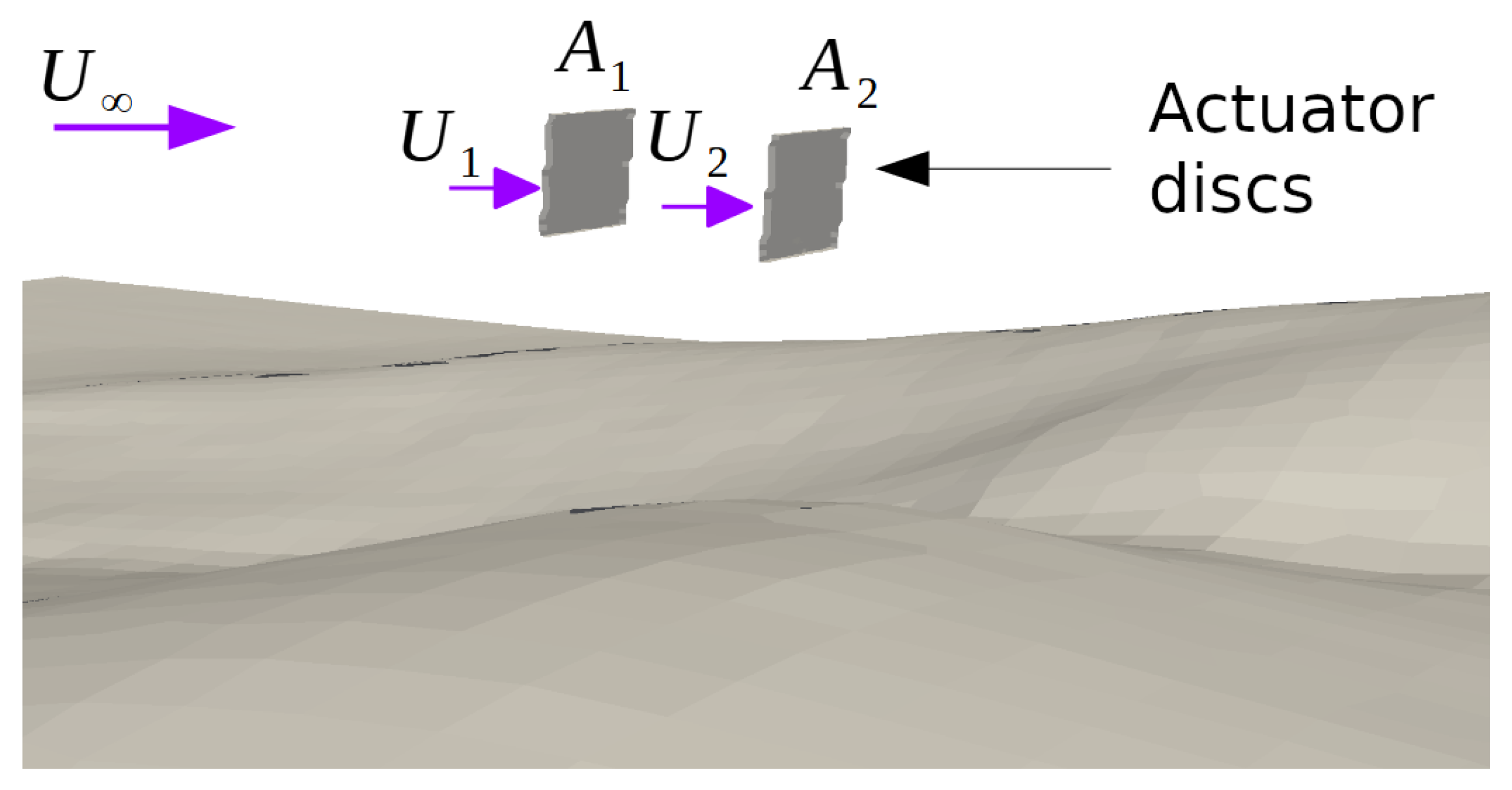
2.1. Mathematical Model

The actuator disc model (ADM) is based on the one-dimensional linear momentum approach and constitutes a basic theory for the calculation of propellers and wind turbines [40,41]. Figure 1 shows the schematic of the flow established around the actuator disc, which is treated as a permeable obstacle with zero thickness. The flow considered is assumed to be inviscid and laminar. Therefore, there is no exchange of momentum and energy through the streamlines that limits the considered flow. It allows for the definition of four characteristic cross-sections and application of the Bernoulli equations and continuity equations. Cross-section 1 is far upstream from the disc with pressure p 1 and velocity U 1 equal to atmospheric pressure and velocity p and U , respectively. Cross-section 2 is in front of the disc, and cross-section 3 is just behind it. Cross-section 4 is far downstream of the disc, where the pressure p 4 is again equal to p after the sudden drop at the disc.
It should be noted that, between cross-sections 2 and 3, where the sudden drop in pressure occurs, the velocity change is continuous. The pressure is rebuilt to the atmospheric pressure p in the wake in cross-section 4, but the wind velocity is lower than the atmospheric velocity U . This loss in wind kinetic energy is equal to the energy transferred from the wind to the disc (wind turbine).
In ADM, the relative change of linear velocity across the disc is called the axial induction factor and is defined as follows:
a = U 1 U 2 U 1
The consequence of the linear momentum theory is the possibility to define the power coefficient C p as a function of the axial induction factor a:
C p = P A D P w = 4 a ( 1 a ) 2
where P A D is the power transmitted by the wind to the actuator disc, and P w = 0.5 ρ A A D U 1 3 is the total power contained in the wind passing through the area equal to the area of the actuator disc A A D .
Similar to the power coefficient, the thrust factor coefficient C T can also be defined as a function of a:
C T = T A D T w = 4 a ( 1 a )
where T A D is the thrust force acting on the disc and T w is the total thrust force contained in the wind acting on the area A A D .
In the present work, the flow of the atmospheric wind was modeled by solving the system of three-dimensional incompressible Navier–Stokes equations:
ρ U t + ρ U U = p + · μ U + i N F i · U = 0
where U = ( U x , U y , U z ) is the velocity vector, p is kinematic pressure, ρ is density of air, and μ is dynamic viscosity of air. The presence of the i-th actuator disc in the flow (i-th wind turbine in a wind farm) was modeled as source terms F i , defined as follows:
F i = 0.5 ρ U Ri 2 A i C T , i = 2 ρ A i U Ri 2 a i 1 a i
where U i is the velocity vector in front of the i-th wind turbine, A i = π R i 2 is the swept area of the turbine, and a i is the axial induction factor of the i-th turbine, which, after applying Equations (2) and (3), can be defined in the following way:
a i = 1 C p , i C T , i
It should be noted that Equation (6) defines a specific wind turbine characterized by its power coefficient C p and thrust force coefficient C T . Consequently, as can be seen in Equation (5) the source term F depends on the characteristics of a wind turbine and the local velocity value, and it is therefore a function of spatial variables and time.
Figure 2 shows the actuator discs that simulate two wind turbines, one behind the other, on an undulating terrain. The characteristics of the actuator discs are described by the source terms (5) and (6). The velocities U R 1 and U R 2 are the wind speeds reaching the corresponding disc, which have swept area A 1 and A 2 , respectively. It is worth noting that any velocity profile can be defined at the inlet, taking into account the roughness of the terrain, any intensity of turbulence, and any (e.g., varying in time or direction) wind speed.
In the classical approach, the values of the power coefficient C p and the thrust force coefficient C T used in Equation (6) are constant. In the current approach, the model (6) was modified to account for variability of these values with respect to atmospheric wind velocity:
a i = 1 C p , i ( U R i ) C T , i ( U R i )
where U R i is the velocity reaching a wind turbine in the i-th row. Due to this, it was possible to use the functional dependencies of C p ( U ) and C T ( U ) for a specific wind turbine. To account for high Reynolds numbers, the k- ϵ turbulence model was used. The k- ϵ model is widely used and accepted for flows with a high Reynolds number where shear effects are of secondary importance and where flow separations do not occur. It is the simplest turbulence model and, therefore, when used properly, provides high convergence and low residuals. In the current research, residues on the order of 10 5 were obtained.

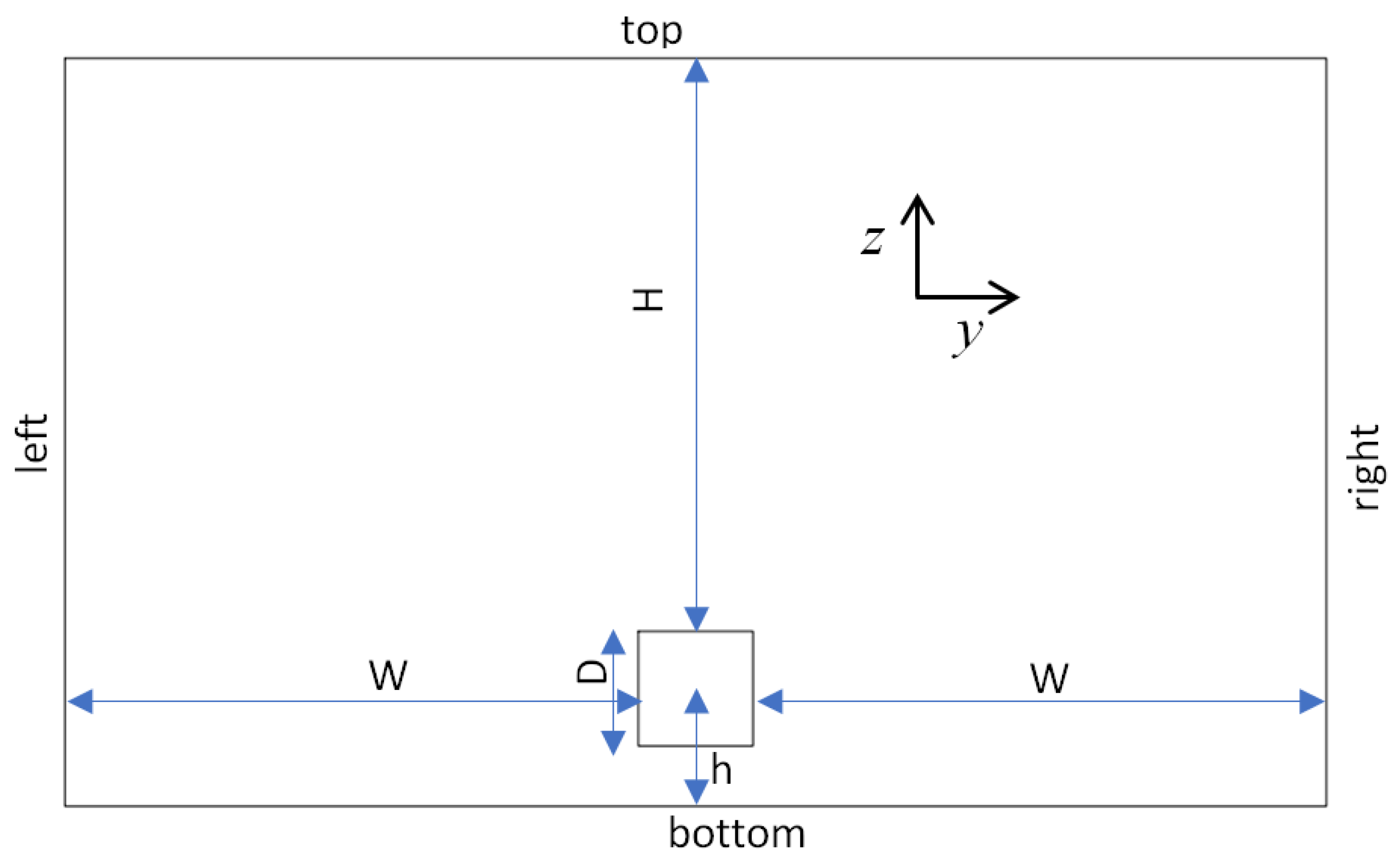
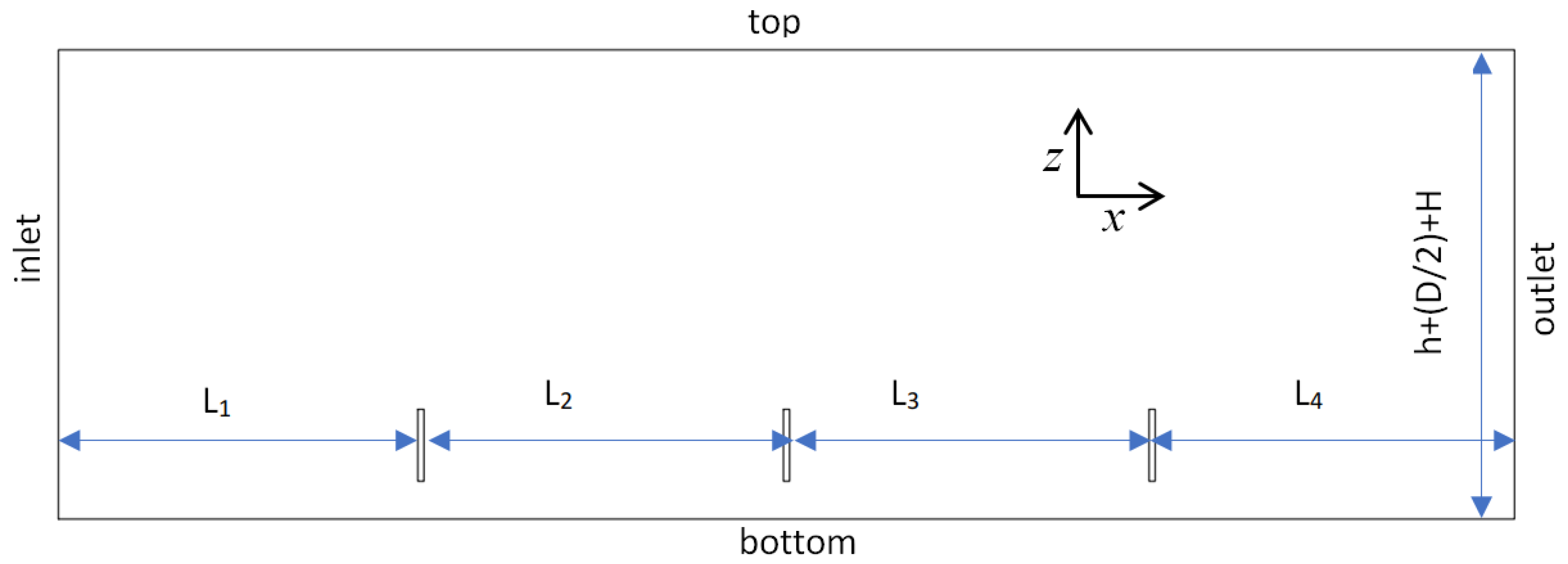
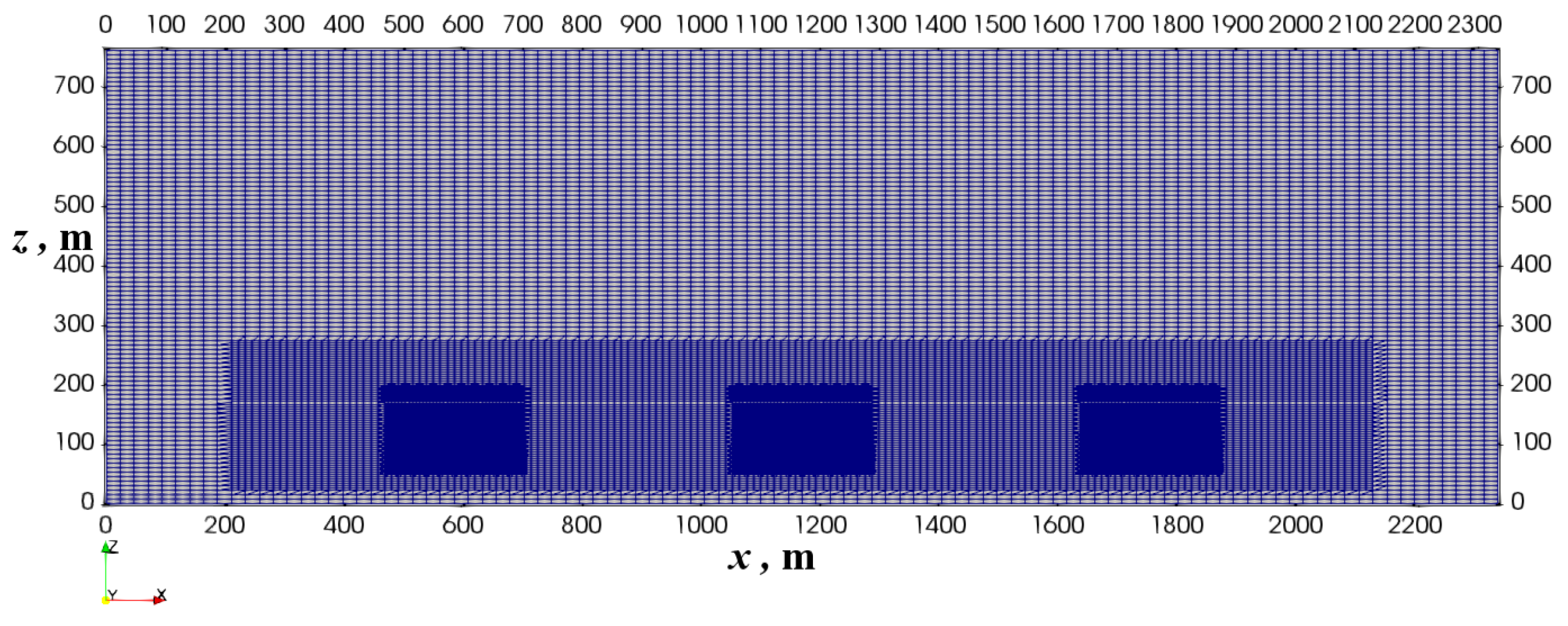
2.2. Numerical Model and Implementation

In the current study, Equations (5) were discretized using the finite volume method (FVM) and solved numerically using the OpenFOAM 7 CFD toolbox (Open Source Field Operation and Manipulation) [42,43] and the SIMPLE algorithm (Semi-Implicit Method for Pressure-Linked Equations) [44,45,46].
The source terms (5) representing wind turbines were defined using the power and trust coefficients C p ( U ) , C T ( U ) and the power curve P W T ( U ) specific to the wind turbine Gamesa G132-5.0MW. The functional dependence of these quantities on the wind velocity U is shown in Figure 3 and the main characteristics of the Gamesa G132-5.0MW turbine are listed in Table 1 [47]. Figure 3 clearly shows that both the coefficients C p and C T of real turbines strongly depend on the value of the wind velocity.
The curves C p ( U ) and C T ( U ) from Figure 3 were approximated using fourth-order polynomials:
C p ( U ) = 1.4462 · 10 5 U 4 + 0.0011 U 3 0.0279 U 2 + 0.254 U 0.2768 C T ( U ) = 1.9334 · 10 5 U 4 + 0.0014 U 3 0.0321 U 2 + 0.2243 U 0.4417
and then used in Equations (5) and (7).
The basic layout of the wind farm considered in the current study is presented in Figure 4 and Figure 5, and all the calculation scenarios considered, including boundary conditions, are shown in Table 2. The consecutive rows in Table 2 number the types of the wind farm (WF) considered:
1.
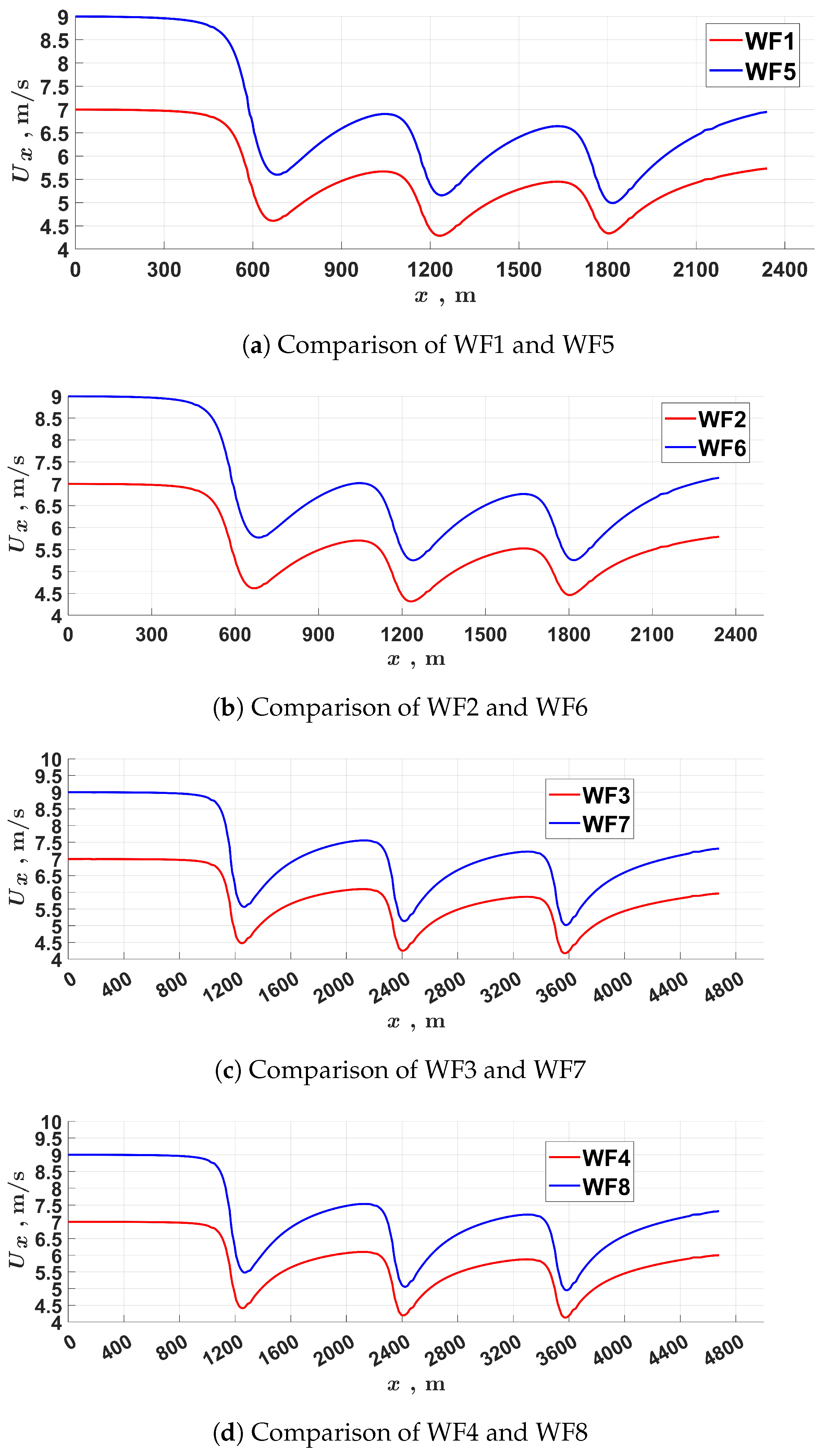
A single column of 3 turbines 5D apart on land (WF1).
2.
A multi-column wind farm composed of 3 rows 5D apart on land (WF2).
3.
A single column of 3 turbines 10D apart on land (WF3).
4.
A multi-column wind farm composed of 3 rows 10D apart on land (WF4).
5.
A single column of 3 turbines 5D apart on sea (WF5).
6.
A multi-column wind farm composed of 3 rows 5D apart on sea (WF6).
7.
A single column of 3 turbines 10D apart on sea (WF7).
8.
A multi-column wind farm composed of 3 rows 10D apart on sea (WF8).
At the inlet, the Atmospheric Boundary Layer (ABL) velocity profile is used, which is defined as follows:
U y = u * κ ln z + z 0 z 0 U x = U z = 0
where u * is the friction velocity, κ = 0.41 is the von Kármán constant, z is the ground-normal coordinate component, and z 0 is roughness length of the terrain. In the current study, two different classes of terrain were considered: land (ABL L ) and sea (ABL S ), for which z 0 = 0.03 m and z 0 = 0.0002 m, respectively. At the outlet (OUT), the standard boundary conditions were used: constant pressure and U n = 0 , where n denotes a normal direction to the boundary. Furthermore, it was assumed that the intensity of turbulence was 10% for the land locations and 1% for the sea locations [7].
The basic structure of a numerical mesh is shown in Figure 6. The use of square shapes to represent the presence of wind turbines in the flow allowed the use of an orthogonal numerical grid consisting of regular cubic elements. This ensured high quality of the numerical mesh, free of skewed and irregular cells.
The mesh was gradually refined in the direction of the turbines and consisted of 3 regions with different levels of refinement. In consecutive regions, the size of the mesh cells was reduced twice. Consequently, their volumes were approximately 1250, 156, and 19.5 m 3 , respectively. The total count of the mesh cell was approximately 3,000,000. In the centers of the areas with the densest mesh, the actuator discs were located.

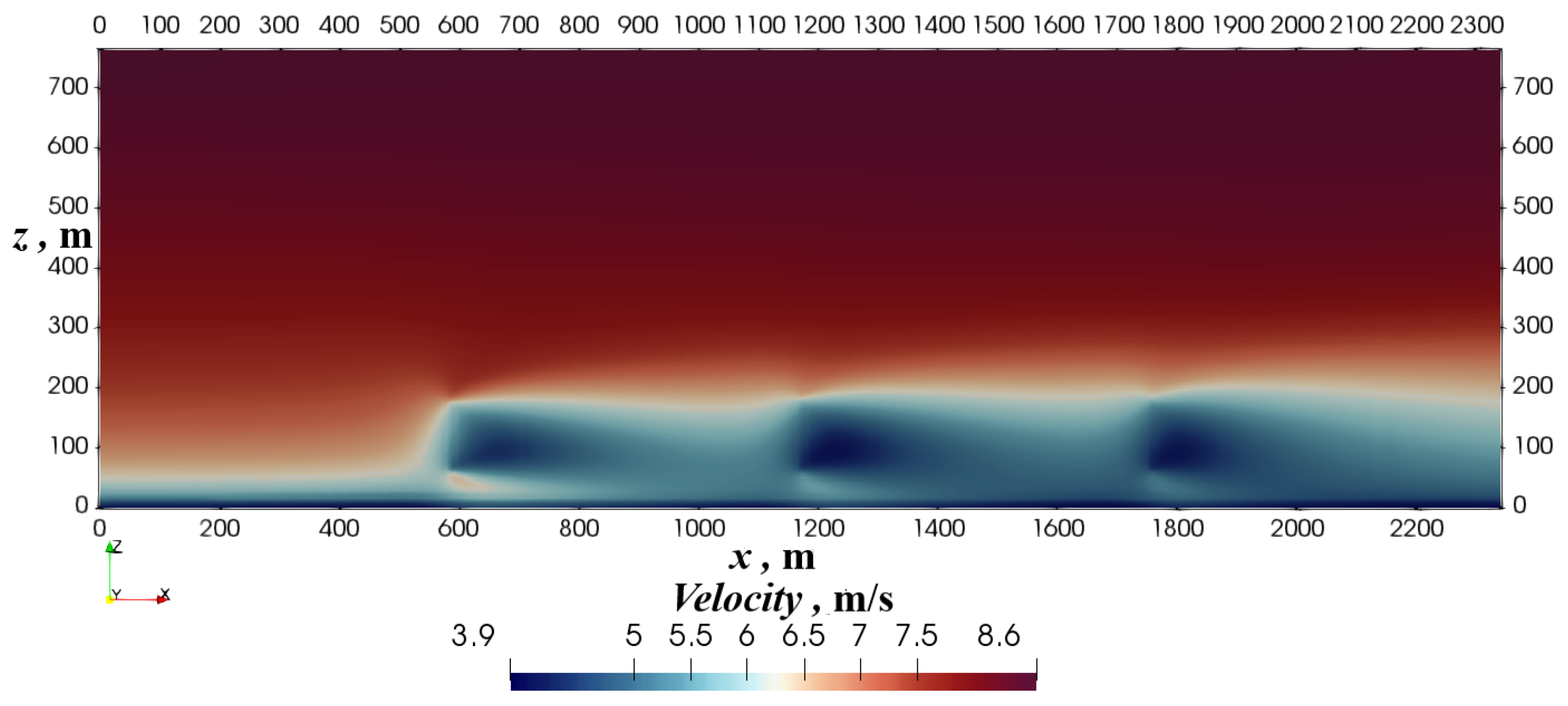
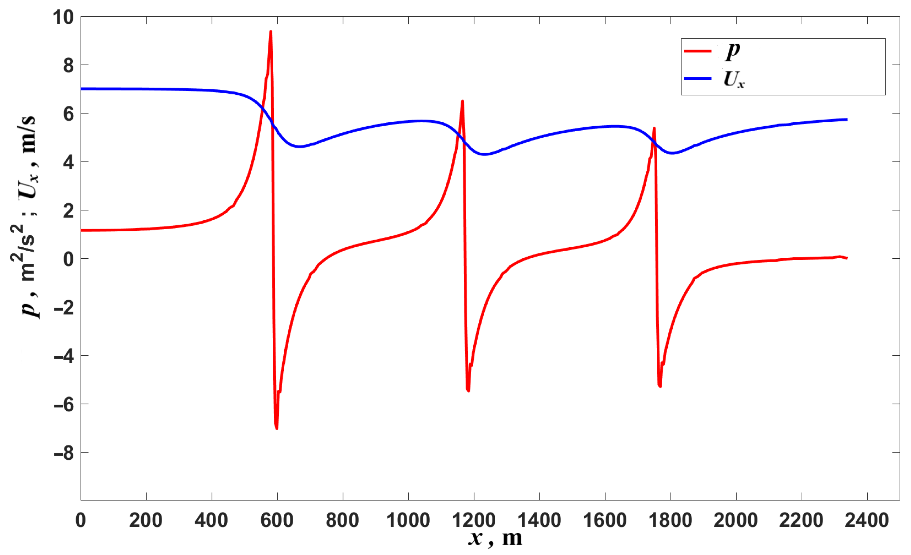
3. Results and Discussion

The aim of this section is to demonstrate the operation of the developed actuator disc model and to discuss the impact of the distance between turbines, atmospheric conditions, and location on the performance of the wind farm.
Figure 7 shows the distribution of the kinematic pressure p for WF number 1. The data presented are taken in the ( x , z ) plane and in the center of the width direction y. It can be seen that overpressure is created at the front of each wind turbine. Furthermore, it can be seen that, downstream of the wind farm, this overpressure decreases. Furthermore, it can be observed that an underpressure is created at the rear of each turbine. As before, the value of the overpressure established behind each turbine decreases down the wind farm. As a consequence, the overall pressure drop across subsequent wind turbines also decreases downstream of the wind farm.
Figure 8 corresponds to Figure 7 and shows the aerodynamic wakes that develop behind each turbine. It can be seen that the wakes overlap, resulting in the velocity deficit becoming larger behind the turbines in subsequent rows. Furthermore, it can be seen that the wakes are approaching the ground and begin to mix with the boundary layer.
The gradual deepening of the velocity deficit is clearly visible in Figure 9, which shows the pressure values and the x component of the velocity U x along the horizontal line that passes through the centers of the consecutive wind turbines. It can be seen that the value of the pressure drop is localized and decreases with each subsequent wind turbine. Moreover, the pressure drop at the first turbine is the largest. Consequently, the velocity drop is the largest at the first turbine as well. More importantly, it can be seen that the distance of 5D between the turbines is too small for the wind velocity to recover to the atmospheric value U . This causes the velocity deficit to deepen down the wind farm. It should be noted that the highest drop in velocity is associated with the highest drop in pressure and occurs after the first row of turbines.
Qualitatively similar behavior is observed for the remaining types of wind farm considered in the study and is listed in Table 2. Table 3 summarizes the results obtained and shows the change in the velocity deficit in each wind farm considered. It can be seen, not surprisingly, that the velocity deficit is larger for smaller distances between turbines (5D), because the velocity cannot be rebuilt before reaching the turbine in the next row. It is worth noting that the velocity deficit is smaller in the case of multi-column wind farms. This happens because the wind speed between wind farm columns may locally increase due to the narrowing of the cross-section of the flow field by the turbine rotors. It is visible in Figure 10, which shows the comparison of the x component of the wind velocity profiles U x in the wake behind the first, second, and third rows of the single-column wind farm (WF1) and the multi-column wind farm (WF2). It can be noticed that the velocity profiles of the multi-column wind farm (WF2) reach slightly higher values both in the wake and away from the turbine in the width y direction. The largest difference can be seen behind the third turbine. Qualitatively similar behavior can be observed when wind farm WF3 is compared with wind farm WF4, when comparing wind farm WF5 with wind farm WF6, and when comparing wind farm WF7 with wind farm WF8.
It should be noted that a greater velocity deficit was observed in the offshore location (wind farms WF5–WF8). This is due to the lower intensity of turbulence in this location compared to land. The consequence of this is less momentum exchange between the wakes and the external flow and a slower recovery of velocity behind the turbines.
The results gathered in Figure 11 summarize the research conducted and show a comparison between the corresponding offshore and onshore wind farms considered in the study. It can be seen that the relative decrease in the value of the velocity deficit in subsequent rows of wind farms is greater in the case of offshore installations. This is related, among other things, to the lower intensity of turbulence for these locations, which causes a slower recovery of the wind velocity behind individual turbines.

Estimation of Losses in Wind Farms

The relative loss (efficiency) η of wind turbines in successive rows compared to the turbine in the first row can be defined as follows:
η i = AEG of WT in i th row AEG of WT in 1 st row
where AEG stands for “Annual Energy Production”. The efficiency of the whole wind farm η W F can be defined as follows:
η W F = AEG of WF ( AEG of isolated turbine ) · N W T
where N W T is the total number of wind turbines in the wind farm under consideration. Consequently, using expression (11), the loss of WF can be calculated as:
ζ W F = 1 η W F
To calculate the loss of energy production ζ W F defined by the expression (12), it is necessary to calculate the AEG, which requires knowledge of the annual variability of the wind speed in a given location. It is generally accepted that this variability can be defined by the Weibull probability density function [41]:
f ( U ) = k U k 1 c k exp U c k
where k is the shape parameter and c is the scale factor defined as:
c = U a v e Γ ( 1 + 1 / k )
where U a v e is the average annual wind velocity at a given location and Γ ( ) is the gamma function. If the value of the shape parameter is not known, k = 2 can be assumed [41]. In the current study, k = 2 was chosen for the location on the land and k = 2.3158 for the offshore location, which is a realistic assumption based on real data [48,49].
It is important to note that the Weibull distribution defined by Equation (13) is only true for the first row of turbines. For subsequent rows, it must be modified due to the existing velocity deficit behind the subsequent rows of turbines. Using the velocity deficit values from Table 3, the probability of a given wind velocity occurring in the distribution should be changed accordingly. Figure 12 shows the probability density function of the wind velocity for the onshore location considered (WF1–WF4) and the modified probability functions for the subsequent rows for WF1. A similar approach was adopted for the other wind farms considered. For the onshore locations, the average velocity U a v e = 7 m/s was assumed, and for the offshore locations, U a v e = 9 m/s.
Finally, the annual electricity generation of the wind turbine in the ith row can be calculated as follows:
AEG i = U c u t i n U c u t o u t f i ( U ) P W T ( U ) d U
where f i ( U ) is the wind probability density function reaching the ith row and U c u t i n , U c u t o u t are the cut-in, cut-out velocities of the considerate turbine, respectively; see Table 1. Consequently, the values of AEG i of each wind turbine can be used to calculate the loss of every turbine using Equation (10). These values are collected in Table 4. By definition, the efficiency of the turbines in the first row η 1 = 1 . The efficiency in the subsequent rows decreases in value and becomes smaller downwind of the wind farm, which is a direct consequence of the observed pressure drop and velocity deficit observed in Figure 7, Figure 8 and Figure 9.
Finally, the annual electricity generation of the entire wind farm can be calculated by summing the individual contributions of each turbine:
AEG W F = i A E G i
The values of AEG W F for the considered wind farms and the corresponding losses are gathered in Table 5. It can be seen that the highest losses are related to the smaller distance between the turbines, which corresponds to the smallest annual energy production. It should be noted that the losses are larger in the case of single-column wind farms, that is, the losses of wind farms WF1, WF3, and WF5 are greater than the losses of WF2, WF4, and WF6.
Table 6 shows the losses of real wind farms, both onshore and offshore. It can be seen that the order of magnitude of the losses recorded in these wind farms is in agreement with the losses obtained in the current study. The relatively large losses recorded at the offshore wind farms of Lillgrund and Scroby Sands are associated with a too-small distance between the wind turbines in the direction of the prevailing wind. In the case of the Lillgrund wind farm, the distance is less than 5D [7].

4. Conclusions

The presented work proposed a modification of the actuator disc model by making it more realistic to real data. The modification was to allow for variability of a power coefficient and a thrust force coefficient by defining them as functions of the atmospheric wind speed. Due to this, the proposed actuator disc model could be used to simulate a specific real wind turbine, characterized by its individual power and thrust force coefficient fictions and for the entire spectrum of wind velocities. It is important especially in the case of wind farms, where the velocity deficit developed in aerodynamic wake behind consecutive rows of turbines is not known beforehand.
The developed model was implemented in the OpenFoam CFD toolbox and used to analyze the interactions of wind turbines and the related losses in electricity production in various configuration of wind farms. The calculations used incompressible three-dimensional Navier–Stokes equations, and the presence of wind turbines in the flow was simulated as additional source terms built on the basis of the proposed actuator disc model.
The calculations presented use the characteristics of a real Gamesa wind turbine with rated power equal to 5 MW. Ten different configurations of wind farms were analyzed, characterized by different distances between turbines (5D and 10D), different number of columns, and different wind conditions corresponding to the location on land and at sea. The velocity deficit was shown to be higher for smaller distances between turbines. It was due to the fact that the velocity was unable to rebuild itself before reaching the turbine in the next row. Furthermore, it was shown that the velocity deficit was smaller in the case of multi-column wind farms. This happened because the wind velocity between the wind farm columns locally increased due to the narrowing of the flow field cross-section caused by the presence of the turbine rotors. Additionally, a greater velocity deficit was observed in the offshore locations. This was due to the lower intensity of turbulence in these locations compared to land locations. The consequence of this was a less intense exchange of momentum between the aerodynamic shadows created behind the wind turbines and the external flow, and consequently, a slower recovery of kinetic energy behind the turbines. Finally, the study showed that the losses in wind farm electricity production could be up to several percent, which was consistent with the losses observed in real wind farms.
The proposed modification of the actuator disc model can be used to analyze wind farm losses, not only in terms of the geometric distribution of individual turbines, but also in terms of a specific type of wind turbine. It can also be used successfully to estimate losses in the case of wind farms consisting of turbines of various types and sizes and throughout the spectrum of wind speeds.

Author Contributions

Conceptualization, Z.M. and G.D.; methodology, Z.M. and G.D.; investigation, Z.M. and G.D.; resources, Z.M. and G.D.; writing—original draft preparation, Z.M. and G.D.; writing—review and editing, Z.M. and G.D.; visualization, G.D.; supervision, Z.M. All authors have read and agreed to the published version of the manuscript.

Funding

The work was financed by the statutory funds of the Department of Cryogenics and Aerospace Engineering of the Wrocław University of Science and Technology.

Data Availability Statement

The data presented in this study are available on request from the corresponding author.

Conflicts of Interest

The authors declare no conflict of interest.

References

  1. GWEC. Global Wind Report 2023; Technical Report; Global Wind Energy Council: Brussels, Belgium, 2023. [Google Scholar]
  2. Ember. Available online: https://ember-climate.org/topics/wind/ (accessed on 18 July 2023).
  3. IRENA. Available online: https://www.irena.org/Energy-Transition/Technology/Wind-energy (accessed on 14 September 2023).
  4. Numerical study of improving Savonius turbine power coefficient by various blade shapes. Alex. Eng. J. 2019, 58, 429–441. [CrossRef]
  5. Beiter, P.; Rand, J.T.; Seel, J.; Lantz, E.; Gilman, P.; Wiser, R. Expert perspectives on the wind plant of the future. Wind Energy 2022, 25, 1363–1378. [Google Scholar] [CrossRef]
  6. Lissaman, P.B.S.; Gyatt, G.W.; Zalay, A. Critical issues in the design and assessment of wind turbine arrays. In Proceedings of the 4th International Symposium on Wind Energy Systems, Stockholm, Sweden, 21 September 1982; Volume 2, pp. 411–423. [Google Scholar]
  7. Malecha, Z. Economic analysis and power capacity factor estimation for an offshore wind farm in the Baltic Sea. Instal 2023, 1, 4–11. (In Polish) [Google Scholar] [CrossRef]
  8. Jedral, W. Generation and storage of large amounts of electricity in the energy transition by 2050. Energetyka Ciepl. Zawodowa 2022, 816, 44–50. (In Polish) [Google Scholar]
  9. Jedral, W. Production of 100% electricity in Poland from RES—A real purpose or utopia? Rynek Energii 2022, 160, 3–15. (In Polish) [Google Scholar]
  10. Jedral, W. Energy storage and hydrogen power engineering in Poland as a result of the power engineering transformation. Rynek Energii 2022, 161, 8–15. (In Polish) [Google Scholar]
  11. Boccard, N. Capacity factor of wind power realized values vs. estimates. Energy Policy 2009, 37, 2679–2688. [Google Scholar] [CrossRef]
  12. White, E.; Kutz, D.; Freels, J.; Monschke, J.; Grife, R.; Sun, Y.; Chao, D. Leading-Edge Roughness Effects on 63(3)-418 Airfoil Performance. In Proceeding of the 49th AIAA Aerospace Sciences Meeting Including the New Horizons Forum and Aerospace Exposition, Orlando, FL, USA, 4–7 January 2011. [Google Scholar] [CrossRef]
  13. Gao, L.; Liu, Y.; Zhou, W.; Hu, H. An experimental study on the aerodynamic performance degradation of a wind turbine blade model induced by ice accretion process. Renew. Energy 2019, 133, 663–675. [Google Scholar] [CrossRef]
  14. Gao, L.; Tao, T.; Liu, Y.; Hu, H. A field study of ice accretion and its effects on the power production of utility-scale wind turbines. Renew. Energy 2021, 167, 917–928. [Google Scholar] [CrossRef]
  15. Corten, G.; Veldkamp, H. Aerodynamics. Insects can halve wind turbine power. Nature 2011, 412, 41–42. [Google Scholar] [CrossRef]
  16. Malecha, Z.; Sierpowski, K. Badania numeryczne wpływu erozji oraz zabrudzeń łopaty na pracę turbiny wiatrowej. Instal 2023, 7–8. [Google Scholar] [CrossRef]
  17. Linnemann, T.; Vallana, G. Wind energy in Germany and Europe Pt 2 Status, potentials and challenges for baseload application: European situation in 2017. Int. Z. Fur. Kernenerg. 2019, 64, 141–148. [Google Scholar]
  18. Gawronska, G.; Gawronski, K.; Król, K.; Gajecka, K. Wind farms in Poland—Legal and location conditions. The case of Margonin wind farm. Gll Geomat. 2019, 3, 25–39. [Google Scholar] [CrossRef]
  19. DTI. Capital Grants Scheme for North Hoyle Offshore Wind Farm; Technical Report; Department of Trade and Industry: London, UK, 2006.
  20. DTI. Capital Grants Scheme for Scroby Sands Offshore Wind Farm; Technical Report; Department of Trade and Industry: London, UK, 2006.
  21. Malecha, Z. Risks for a Successful Transition to a Net-Zero Emissions Energy System. Energies 2022, 15, 4071. [Google Scholar] [CrossRef]
  22. Hansen, K.S.; Barthelmie, R.J.; Jensen, L.E.; Sommer, A. The impact of turbulence intensity and atmospheric stability on power deficits due to wind turbine wakes at Horns Rev wind farm. Wind Energy 2012, 15, 183–196. [Google Scholar] [CrossRef]
  23. Dahlberg, J.; Thor, S. Power Performance and Wake Effects in the Closely Spaced Lillgrund Offshore Wind Farm. In Proceedings of the European Offshore Wind 2009 Conference and Exhibition, Stockholm, Sweden, 14–16 September 2009. [Google Scholar]
  24. Sørensen, T.; Thøgersen, M.L. Recalibrating Wind Turbine Wake Model Parameters—Validating the Wake Model Performance for Large Offshore Wind Farms. In Proceedings of the European Wind Energy Conference and Exhibition, Athens, Greece, 27 February–2 March 2006. [Google Scholar]
  25. Lee, M.; Keith, D. Climatic Impacts of Wind Power. Joule 2018, 2, 2618–2632. [Google Scholar] [CrossRef]
  26. Harris, R.A.; Zhou, L.; Xia, G. Satellite Observations of Wind Farm Impacts on Nocturnal Land Surface Temperature in Iowa. Remote. Sens. 2014, 6, 12234–12246. [Google Scholar] [CrossRef]
  27. Slawsky, L.M.; Zhou, L.; Roy, S.B.; Xia, G.; Vuille, M.; Harris, R.A. Observed Thermal Impacts of Wind Farms over Northern Illinois. Sensors 2015, 15, 14981–15005. [Google Scholar] [CrossRef]
  28. Smith, C.M.; Barthelmie, R.J.; Pryor, S.C. In situ observations of the influence of a large onshore wind farm on near-surface temperature, turbulence intensity and wind speed profiles. Environ. Res. Lett. 2013, 8, 034006. [Google Scholar] [CrossRef]
  29. Zhou, L.; Tian, Y.; Baidya Roy, S.; Thorncroft, C.; Bosart, L.F.; Hu, Y. Impacts of wind farms on land surface temperature. Nat. Clim. Chang. 2012, 2, 539–543. [Google Scholar] [CrossRef]
  30. Zhou, L.; Tian, Y.; Baidya Roy, S.; Dai, Y.; Chen, H. Diurnal and seasonal variations of wind farm impacts on land surface temperature over western Texas. Nat. Clim. Chang. 2013, 41, 307–326. [Google Scholar] [CrossRef]
  31. Jacobson, M.; Delucchi, M.; Cameron, M.; Mathiesen, B. Matching demand with supply at low cost in 139 countries among 20 world regions with 100% intermittent wind, water, and sunlight (WWS) for all purposes. Renew. Energy 2018, 123, 236–248. [Google Scholar] [CrossRef]
  32. Jacobson, M.Z.; Archer, C.L. Saturation wind power potential and its implications for wind energy. Proc. Natl. Acad. Sci. USA 2012, 109, 15679–15684. [Google Scholar] [CrossRef]
  33. Jensen, N. A Note on Wind Generator Interaction; Number 2411 in Risø-M; Risø National Laboratory: Roskilde, Denmark, 1983. [Google Scholar]
  34. Katic, I.; Højstrup, J.; Jensen, N. A Simple Model for Cluster Efficiency. In EWEC’86. Proceedings. Vol. 1, Proceedings of the European Wind Energy Association Conference and Exhibition, Rome, Italy, 8–10 October 1986; Palz, W., Sesto, E., Eds.; A. Raguzzi: Rome, Italy, 1987; pp. 407–410. [Google Scholar]
  35. Göçmen, T.; van der Laan, P.; Réthoré, P.E.; Diaz, A.P.; Larsen, G.C.; Ott, S. Wind turbine wake models developed at the technical university of Denmark: A review. Renew. Sustain. Energy Rev. 2016, 60, 752–769. [Google Scholar] [CrossRef]
  36. Peña, A.; Réthoré, P.E.; van der Laan, M.P. On the application of the Jensen wake model using a turbulence-dependent wake decay coefficient: The Sexbierum case. Wind Energy 2015, 19, 763–776. [Google Scholar] [CrossRef]
  37. Sørensen, J. 2.08-Aerodynamic Analysis of Wind Turbines. In Comprehensive Renewable Energy; Sayigh, A., Ed.; Elsevier: Oxford, UK, 2012; pp. 225–241. [Google Scholar] [CrossRef]
  38. Martinez, L.; Leonardi, S.; Churchfield, M.; Moriarty, P. A Comparison of Actuator Disk and Actuator Line Wind Turbine Models and Best Practices for Their Use. In Proceedings of the 50th AIAA Aerospace Sciences Meeting including the New Horizons Forum and Aerospace Exposition, Nashville, Tennessee, 9–12 January 2012. [Google Scholar] [CrossRef]
  39. Richmond, M.; Antoniadis, A.; Wang, L.; Kolios, A.; Al-Sanad, S.; Parol, J. Evaluation of an offshore wind farm computational fluid dynamics model against operational site data. Ocean. Eng. 2019, 193, 106579. [Google Scholar] [CrossRef]
  40. Manwell, J.F.; McGowan, J.G.; Rogers, A.L. Wind Energy Explained: Theory, Design and Application; John Wiley & Sons: Hoboken, NJ, USA, 2010. [Google Scholar]
  41. Burton, T.; Jenkins, N.; Sharpe, D.; Bossanyi, E. Wind Energy Handbook; John Wiley & Sons: Hoboken, NJ, USA, 2011. [Google Scholar]
  42. OpenFoam and OpenCFD. Available online: https://www.openfoam.com/ (accessed on 22 April 2023).
  43. OpenFOAM and The OpenFOAM Foundation. Available online: https://www.openfoam.org/ (accessed on 22 April 2023).
  44. Issa, R.; Gosman, A.; Watkins, A. The computation of compressible and incompressible recirculating flows by a non-iterative implicit scheme. J. Comput. Phys. 1986, 62, 66–82. [Google Scholar] [CrossRef]
  45. Ferziger, J.H.; Peric, M.; Street, R.L. Computational Methods for Fluid Dynamics; Springer: Cham, Switzerland, 2020. [Google Scholar] [CrossRef]
  46. Moukalled, F.; Mangani, L.; Darwish, M. The Finite Volume Method in Computational Fluid Dynamics: An Advanced Introduction with OpenFOAM and Matlab; Springer: Cham, Switzerland, 2015. [Google Scholar] [CrossRef]
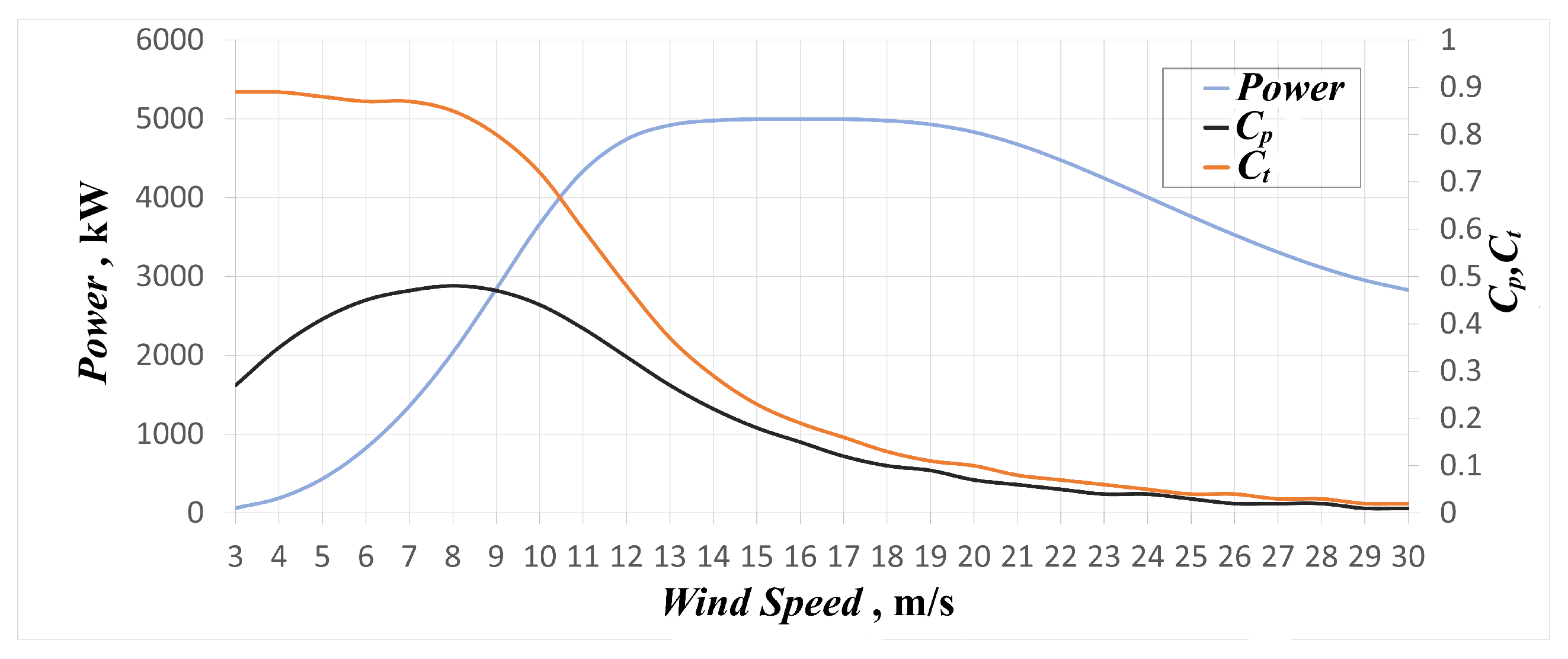
  47. Wind-Turbine-Models. Available online: https://en.wind-turbine-models.com/turbines/768-gamesa-g132-5.0mw#datasheet (accessed on 14 September 2023).
  48. Dailidiene, I.; Baudler, H.; Chubarenko, B.; Navrotskaya, S. Long term water level and surface temperature changes in the lagoons of the southern and eastern Baltic. Oceanologia 2011, 53, 293–308. [Google Scholar] [CrossRef]
  49. Svensson, N.; Arnqvist, J.; Bergström, H.; Rutgersson, A.; Sahlée, E. Measurements and Modelling of Offshore Wind Profiles in a Semi-Enclosed Sea. Atmosphere 2019, 10, 194. [Google Scholar] [CrossRef]
  50. Dahlberg, J.A.; Thor, S.E. Power performance and wake effects in the closely spaced Lillgrund offshore wind farm. In Proceedings of the European Offshore Wind 2009 Conference and Exhibition, Stockholm, Sweden, 14–16 September 2009; p. 1. [Google Scholar]
Figure 1. Sketch of the actuator disc model concept. Numbers 1, 2, 3, and 4 show the locations of the characteristic cross-sections used in linear momentum theory.
Computation 11 00213 g001
Figure 2. Actuator discs simulating two wind turbines placed one behind the other over rugged terrain. The characteristics of the turbines are described by the Equations (5) and (6). Calculation example taken from [42,43].
Computation 11 00213 g002
Figure 3. Power curve P W T ( U ) , C p ( U ) , and C T ( U ) of the Gamesa G132-5.0MW turbine considered in the current study [47].
Computation 11 00213 g003
Figure 4. Front view ( y , z plane) of the placement of the actuator disc, dimensions, and boundaries.
Computation 11 00213 g004
Figure 5. Side view ( x , z plane) of the placement of the actuator discs, dimensions, and boundaries.
Computation 11 00213 g005
Figure 6. Numerical mesh detail with visibility of three levels of refinement. The actuator discs are located in the center of the region with the finest mesh.
Computation 11 00213 g006
Figure 7. Kinematic pressure distribution in the ( x , z ) plane at y = W + 0.5 D for WF number 1.
Computation 11 00213 g007
Figure 8. Velocity magnitude distribution in the ( x , z ) plane at y = W + 0.5 D for WF number 1.
Computation 11 00213 g008
Figure 9. Kinematic pressure and x component of velocity distribution along a line parallel to the x axis and passing through the center of the discs for WF number 1.
Computation 11 00213 g009
Figure 10. Comparison of the velocity profiles in the wake between the single-column wind farm WF1 and multi-column wind farm WF2. The plots are taken in the direction of the width direction y just behind the actuator discs and at the height z = 120 m (the hub height).
Computation 11 00213 g010
Figure 11. Comparison of U x velocity between the corresponding onshore and offshore wind farms (see Table 2). Plots are taken along the line that goes through the centers of the actuator discs.
Computation 11 00213 g011
Figure 12. Weibull wind velocity probability distribution for the onshore location and modified wind velocity distributions reaching the turbines in subsequent rows. Data for WF1.
Computation 11 00213 g012
Table 1. Main characteristics of the Gamesa G132-5.0MW turbine.
Cut-in speed U c u t i n 3 m/s
Cut-out speed U c u t o u t 27 m/s
Rotor diameter R132 m
Swept area13,685 m 2
Hub height120 m
Table 2. Considered cases of the wind farm (WF) layouts and corresponding boundary conditions.
WFL 1 , 4 L 2 , 3 WHInletOutletLeftRightTopBottom
15D5D5D5DABL L OUTslipslipslipnoslip
25D5D2.5D5DABL L OUTcycliccyclicslipnoslip
310D10D10D5DABL L OUTslipslipslipnoslip
410D10D5D10DABL L OUTcycliccyclicslipnoslip
55D5D5D5DABL S OUTslipslipslipnoslip
65D5D2.5D5DABL S OUTcycliccyclicslipnoslip
710D10D10D5DABL S OUTslipslipslipnoslip
810D10D5D10DABL S OUTcycliccyclicslipnoslip
Table 3. Velocity deficit in front of the first, second, and third row of turbines; U = ( 7 , 9 ) m/s at the reference height z r e f = h = 120 m, for the onshore and offshore WF, respectively.
WF U R 1 / U U R 2 / U U R 3 / U
10.84670.7260.6868
20.84950.7320.7005
30.87460.78330.7559
40.87720.78640.7598
50.8690.69910.6827
60.85130.70490.6654
70.87470.75770.7256
80.87730.75960.7286
Table 4. Efficiency η of very turbine for every considered WF.
WF η 1 η 2 η 3
110.8970.840
210.9000.849
310.9260.886
410.9270.888
510.8800.831
610.8930.838
710.9180.876
810.9180.876
Table 5. Annual electricity production of the considered WF and corresponding losses.
WFAEG WF ζ WF
GWh%
12630.516.0
22671.215.1
32907.911.4
42925.211.2
53033.316.9
62982.716.2
73221.512.4
83234.612.4
Table 6. Losses ζ W F of existing wind farms; P R is the rated power of turbine [7,18,22,24,50].
WF ζ WF Turbine Type
Lillgrund
offshore
0.23Siemens SWT-2.3-93
P R = 2.3 MW
Horns Rev
offshore
0.124Vestas V80
P R = 2 MW
Margonin
onshore
0.2Gamesa G90
P R = 2 MW
Scroby Sands
offshore
0.385Vestas V80
P R = 2 MW
North Hoyle
offshore
0.15Vestas V80
P R = 2 MW
Disclaimer/Publisher’s Note: The statements, opinions and data contained in all publications are solely those of the individual author(s) and contributor(s) and not of MDPI and/or the editor(s). MDPI and/or the editor(s) disclaim responsibility for any injury to people or property resulting from any ideas, methods, instructions or products referred to in the content.

