Transformer-Based Model for Predicting Customers’ Next Purchase Day in e-Commerce

Abstract

The paper focuses on predicting the next purchase day (NPD) for customers in e-commerce, a task with applications in marketing, inventory management, and customer retention. A novel transformer-based model for NPD prediction is introduced and compared to traditional methods such as ARIMA, XGBoost, and LSTM. Transformers offer advantages in capturing long-term dependencies within time series data through self-attention mechanisms. This adaptability to various time series patterns, including trends, seasonality, and irregularities, makes them a promising choice for NPD prediction. The transformer model demonstrates improvements in prediction accuracy compared to the baselines. Additionally, a clustered transformer model is proposed, which further enhances accuracy, emphasizing the potential of this architecture for NPD prediction.

1. Introduction

E-commerce is an important category of websites that help in connecting businesses with their customers. These platforms are constantly improving in order to meet the needs of customers. E-commerce represents a virtual store where customers can search, compare, and buy their favorite products from the comfort of their homes or on the go. Another important advantage is removing geographical barriers, helping businesses to have larger audiences and customers to get products that were not previously accessible without travelling to that location. By having a digital presence, companies can target customers more efficiently and understand their behavior when it comes to purchasing products. E-commerce has also created new buying trends, such as subscription models or personalized experiences [1].

Customer behavior is analyzed by e-commerce businesses to understand how their platform is used and what habits their customers have. User actions, purchases, trends, and preferences are used to gain valuable insights into their behavior. The analysis usually starts from the moment a customer lands on the website until their final purchase decision. Every click, search query, and scroll can provide important information. Using the insights generated from these, companies can create product recommendations and marketing campaigns that are helpful for both the customer and business. Another important aspect is determining the churn rate. This includes the abandoned shopping carts, lack of stock, reviews, and ratings, allowing companies to adjust their platform to fit their customers’ needs. Studying consumer behavior is necessary for understanding the combination of requirements, expectations, and driving factors that influence customers [2].

There are multiple metrics that companies use to track their user behavior. These include conversion rate, average order value, customer lifetime value, customer acquisition costs, or others. These give businesses quantitative information about a variety of areas of their operations, such as sales, customer acquisition, and marketing performance. In this way, businesses can make data-driven decisions that have a solid foundation and remain flexible on small changes that occur depending on the market conditions and their customers’ behavior [3].

Another important metric that is harder to determine because it involves predicting the future values is the customer’s next purchase day (NPD). It is often overlooked because of the need for past data and algorithms that can help determine this value. NPD represents the predicted date when a customer is most likely to make a new purchase. Using the purchase data for each customer, a linear or machine learning model can successfully estimate when the customer will make the next purchase [4].

While the NPD metric can be used in multiple domains, such as “Software as a Service” (SaaS) products, financial services, hospitality, and supply chain management, the scope of this study is limited to e-commerce stores to better understand its characteristics and importance. Improving the method on an initial problem can be beneficial in generalizing a solution that can be used in multiple domains.

Predicting the NPD is addressed as a time series forecasting problem. The sequential purchases of each customer from e-commerce stores create a time series for the prediction task. The forecasting models usually require a significant amount of past data to estimate the future values. E-commerce platforms store these data internally, which can be used in predicting the NPD [5].

Knowing this metric can be used in multiple applications. For example, in targeted marketing, the NPD metric can be used to reach only the customers most likely to buy in the next period, optimizing the campaign budget. In revenue forecasting, the businesses can estimate future revenue using the number of customers that will purchase products as external information in the model. In customer lifetime value, businesses can better estimate and improve the future value of customers by determining their NPD, which can help in acquisition costs and determining the required marketing budgets.

The main contribution in this article is defining an architecture for predicting the NPD for customers of e-commerce stores. A transformer model is proposed to be used for the prediction, which is compared with baseline models used in other studies.

The rest of the paper is structured as follows. Section 2 includes relevant related work in the domain of time series forecasting and customers’ NPD. Section 3 presents the proposed transformer model and the architecture for determining the NPD. Section 4 shows the experimental results in terms of the effectiveness of the models when solving the NPD problem. The last section contains the conclusions and future work for improving the model.

2. Related Work

Predicting consumer behavior in e-commerce has attracted interest from businesses and academia. This section reviews the related work in the area of customers’ NPD prediction, focusing on time series forecasting models.

In [6], the NPD of customers from e-commerce websites is predicted using several methods, such as random forest (RF), autoregressive integrated moving average (ARIMA), convolutional neural network (CNN), and multilayer perceptron (MLP). The authors proposed a deep learning method based on long short-term memory (LSTM) networks. The model has two LSTM layers with sixteen neurons each. The authors test and compare the proposed model with RF, ARIMA, CNN, and MLP using a retail market dataset. While the model outperforms the alternative techniques in this study, it is shown that LSTMs have difficulty handling very long sequences due to the vanishing gradient problem, and scaling to larger datasets because of the lack of parallelization and sensitivity to hyperparameters. The studies [5,7] also determine the NPD for a customer on specific products using machine learning models, such as linear regression, XGBoost, ANNs, and RNNs. It uses the Cross Industry Standard Process for Data Mining (CRISP-DM) for building the solution to a feasible NPD predictor. A combination of methods are used, such as ANN with extreme gradient boosting (XGBoost), ANN with Recurrent Neural Network (RNN), and XGBoost with RNN. Overall, the ANN outperforms the individual models and the combinations of models with an error of less than 1–2 days and is selected for the final solution. ANNs are versatile for a large number of problems, but have limitations when handling sequential data, such as not taking into account positional information and lacking inherent memory, unlike RNNs.

Analyzing the papers that address the NPD problem, the usage of the same known methods for time series forecasting is observed. This leaves a gap for predicting the NPD with more efficient methods that handle sequential data. The following studies address different problems than NPD, but with more varied methods that show improvements in forecasting the specified datasets.

Thus, in a different context than NPD prediction, ref. [8] compares ARIMA, LSTM and Prophet models for time series forecasting in the case of oil production datasets. ARIMA is found to be suitable for short-term predictions, while LSTM and Prophet excel in capturing unusual production changes. The Prophet model reveals potential seasonal effects. When extended to predict oil production across multiple wells in unconventional reservoirs, ARIMA and LSTM outperforms Prophet, suggesting the absence of seasonality in certain oil production curves.

Some hybrid approaches integrating deep learning models with statistical features extracted from the input data are described in [9]. They involve two stages: feature computation and XGBoost-based model fitting in the first stage, and training deep neural networks using original and feature-based samples in the second stage. Three deep learning methods, temporal convolutional networks (TCN), Multi-head Attention, and Multi-head-Attention-Res, are combined with XGBoost to create XGBoost-TCN, XGBoost-ATT, and XGBoost-ATT-Res models. The results on renewable energy consumption datasets reveal that the combined models outperform regular variants and seem to be superior to existing time series forecasting models, which demonstrates the effectiveness of integrating side information with input data for improved predictions.

The experiments performed in [10] also highlight the effectiveness of using hybrid approaches by combining two sub-optimal models: ARIMA and XGBoost. This demonstrates that a fusion can produce forecasts comparable to or better than highly optimized models, in a significantly reduced computation time. Through extensive testing on over 4000 real-life time series, the hybrid method consistently delivers forecasts surpassing a heavily optimized ARIMA model while utilizing only around 25% of the computational resources. Furthermore, it outperformed the simpler ARIMA model with just a negligible increase in computational time. This underscores the importance of not only prioritizing forecasting accuracy but also considering advancements in speed and computational efficiency as time series forecasting gains prominence across diverse business domains and at increasingly granular levels.

The transformer architecture with its attention mechanism is used by researchers in different forecasting problems. By analyzing the production history of three wells, ref. [11] proposes a data-driven approach using an attention mechanism combined with a LSTM network (A-LSTM). This proves highly accurate and versatile; the combination significantly improves accuracy and accommodates noisy data well. It shows the stability, feasibility, and cost-efficiency of the A-LSTM compared to various other models, and it emphasizes A-LSTM as a powerful tool for production forecasting, promising valuable insights for engineers and operators in the oil and gas sector.

The research conducted in [12] addresses the need for accurate time series forecasting in diverse domains such as energy planning, epidemic prevention, and financial analysis. It identifies challenges tied to cumulative errors in autoregressive models for long-term forecasting and the complexity of temporal patterns. The proposed solution is a hierarchical transformer with a probabilistic decomposition representation, integrating the transformer with a conditional generative model based on variational inference. This hierarchical approach effectively mitigates cumulative errors by imposing sequence-level constraints and enables the separation of temporal patterns for enhanced interpretability and prediction accuracy. The evaluation of multiple time series datasets shows the superior accuracy of the method compared to state-of-the-art approaches. Ablation experiments confirm the effectiveness and robustness of the probabilistic decomposition block, establishing this method as a reliable alternative for time series probabilistic forecasting.

A transformer model is also used in [13] for predicting potential floods with a lead time of one day in advance. The utilized model slightly differs from the original implementation in [14]; the absence of decoder layers is the primary distinction. As a result, it uses just encoder layers and directly translates the extracted representations to the output value. The transformer outperforms both LSTM and gated recurrent unit (GRU) neural networks, which are used as benchmarks in the experiments.

While many research papers show that transformers offer better results than RNNs, ref. [15] challenges the efficiency of transformers for long time series forecasting. It demonstrates that a linear model can offer slightly better results than transformer-based methods, such as autoformer or informer.

3. The Proposed Model

To estimate when a consumer is likely to make their next purchase, data analysis and machine learning techniques are used to predict the next purchase day of clients in e-commerce stores. The steps for generating the NPD are presented as follows [16].

Data gathering. The necessary data about the customers are gathered from the e-commerce platform. Historical transaction data are required, which include dates of purchases, customer IDs, product categories, order values, and customer demographics. The data need to be cleaned to make sure they are accurate and in a usable format. Managing missing values, eliminating outliers, and transforming categorical variables into numerical representation using methods like one-hot encoding may be required. Other features that help in determining the day of the upcoming transaction are recency (the number of days since the customer’s last purchase) and frequency (the number of purchases made by the customer).

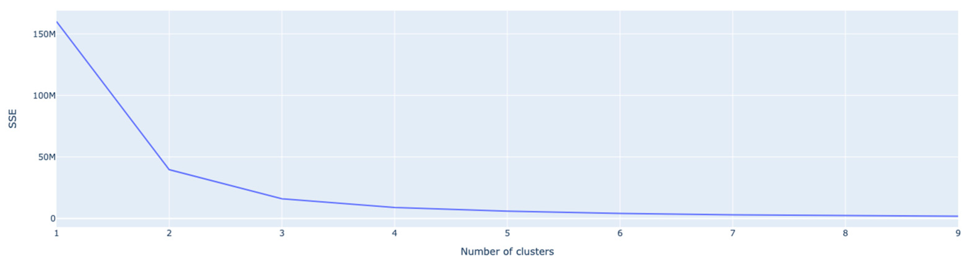
Clustering. Grouping customers that have similar buying patterns can be used to create a more accurate model. The unsupervised k-means clustering algorithm can be used for this purpose, i.e., to divide the dataset into a predetermined number of clusters. The procedure starts with choosing the appropriate number of clusters k and randomly initializing the centroid of each cluster. The next step is to assign each data point to the closest centroid using a predefined distance metric, usually the Euclidean distance. The algorithm then computes a new mean for the data points given to each cluster in order to update the centroids. This assignment–update cycle continues repeatedly until the centroids stabilize or a predetermined number of iterations is reached. For good results, selecting the ideal number of clusters is essential, as well as taking into account how sensitive the algorithm is to the original centroid placement. The number of clusters can be selected using the elbow method [17].

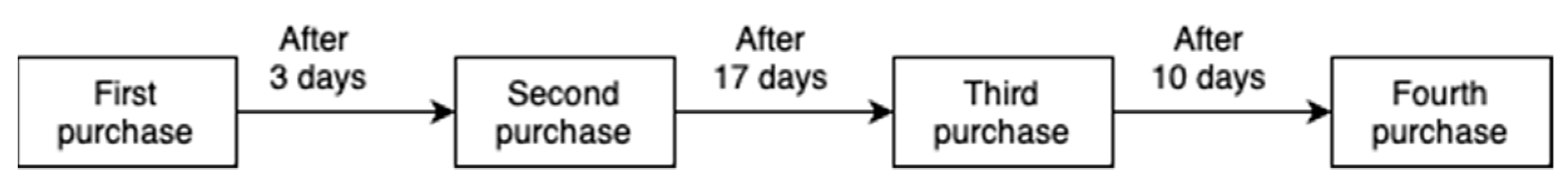
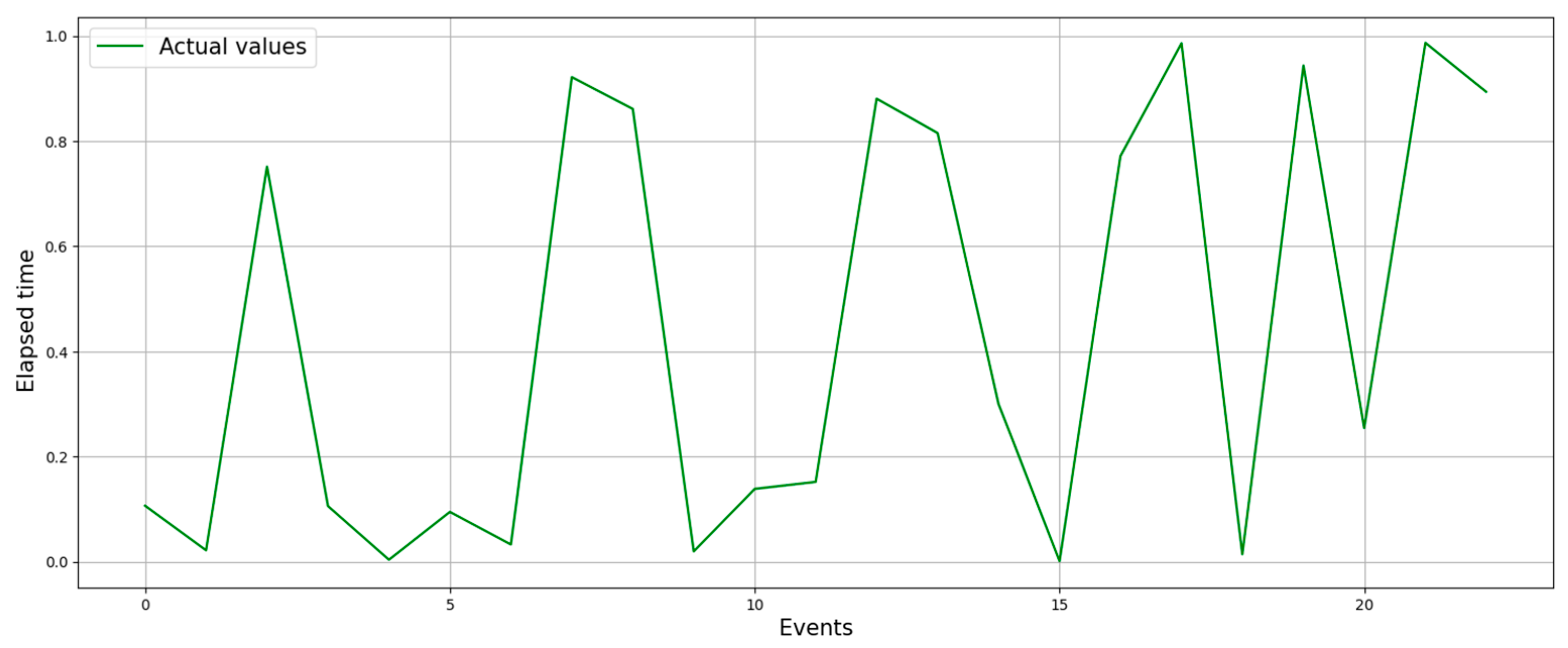
Data pre-processing. A feature that represents the elapsed time between purchases is generated from the customer purchases dataset. The days between orders, exemplified in Figure 1, are calculated for each customer by taking the date difference between two consecutive purchases.

Figure 1. Days between orders feature generation (adapted after [5]).

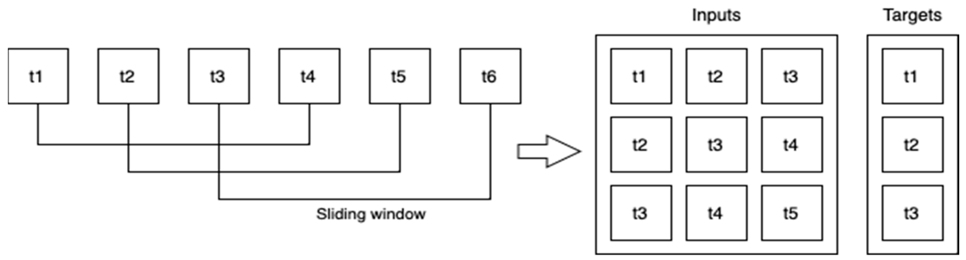
The sequential time series data are converted to be used in a supervised learning model. A sliding window approach is used, as shown in Figure 2. The values from the most recent time steps are used to estimate the value in the following time step. Partitioning the time series data into overlapping subsequences and selecting a portion for training and another for testing are necessary for the creation of a training–testing split.

Figure 2. Converting the time series data into a supervised learning problem (adapted after [18]).

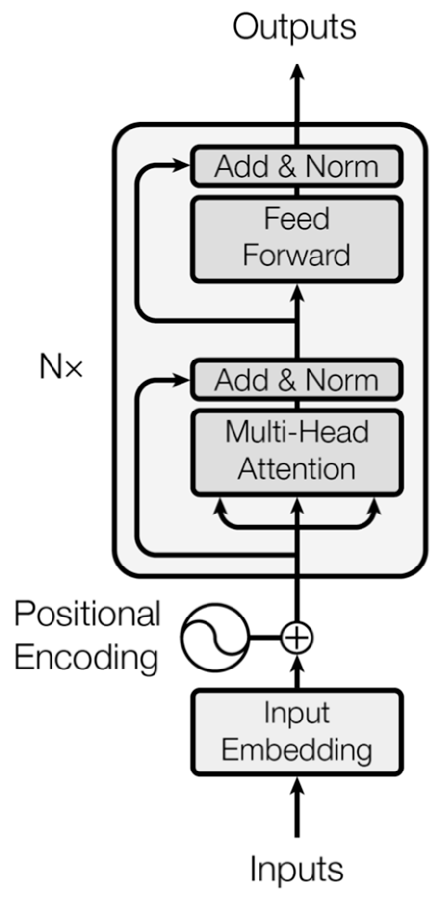
Model training. Training a time series forecasting model with a transformer involves a structured series of steps. Data are transformed using tokenization and normalization into an appropriate format. The model architecture is defined by selecting the number of encoder and decoder layers, attention heads, feedforward network dimensions, and other important hyperparameters, as shown in Figure 3. The proposed model uses only encoder layers to offer the best results with the lowest computation time. Positional encodings are included to provide positional information to the model. Regularization methods used to prevent overfitting and improve generalization are dropout and layer normalization. The effectiveness of the model is determined using the mean square error (MSE) loss function. During training, the weights of the model are adjusted to minimize the loss function using the Adam optimizer.

Figure 3. The proposed transformer architecture (adapted from [14]).

The model representations of the encoder layers are mapped directly to the outputs. The model returns a single prediction. After model training, the generalization and predictions of the model are assessed using a test dataset. A set of evaluation metrics is used to compare the predictions of the model for the target time series to the actual ground truth values: root mean square error (RMSE) and mean absolute error (MAE). The precision, accuracy, and deviation of the predictions from the actual values are all quantified by these metrics. Better model performance is indicated by the lower values of these indicators. A qualitative evaluation of the predicting ability of the model can be provided by visualizations such time series plots that overlay actual and expected values.

Model architecture. While other studies focus on well-known models for time series forecasting, this article focuses on using a recent transformer model used especially in large language models. It is based on the transformer model proposed by [14]. The pseudocode of the proposed technique is presented in Pseudocode 1.

• Pseudocode 1. The workflow using the transformer model.

input data frame with the e-commerce store purchase history determine the number of clusters k and apply k-means to group data into k clusters filter data and select the min threshold for frequency of purchases for each cluster:   for each customer in cluster:      create the time series with time differences between consecutive purchases   create the dataset with the time series of customers in the cluster   train the transformer model for each customer:      predict the next purchase day

4. Experiments

4.1. Dataset

The dataset used is the “Online Retail Data Set” [19]. It has details about 5942 online customers from 43 different nations. The available information is invoice number, stock code, description, quantity, invoice date, unit price, customer ID, and country. This is presented in Table 1. The main elements used are customer ID and invoice date.

Table 1. Online retail dataset structure (showing four examples of purchases).

	Invoice No.	Stock Code	Description	Quantity	Invoice Date	Unit Price	Customer ID	Country
1	489434	85048	15 cm Christmas Glass Ball 20 Lights	12	1 December 2009 07:45:00	6.95	13085	United Kingdom
2	489434	79323P	Pink Cherry Lights	12	1 December 2009 07:45:00	6.75	13085	United Kingdom
3	489434	79323W	White Cherry Lights	12	1 December 2009 07:45:00	6.75	13085	United Kingdom
4	489434	22041	Record Frame 7” Single Size	48	1 December 2009 07:45:00	2.10	13085	United Kingdom

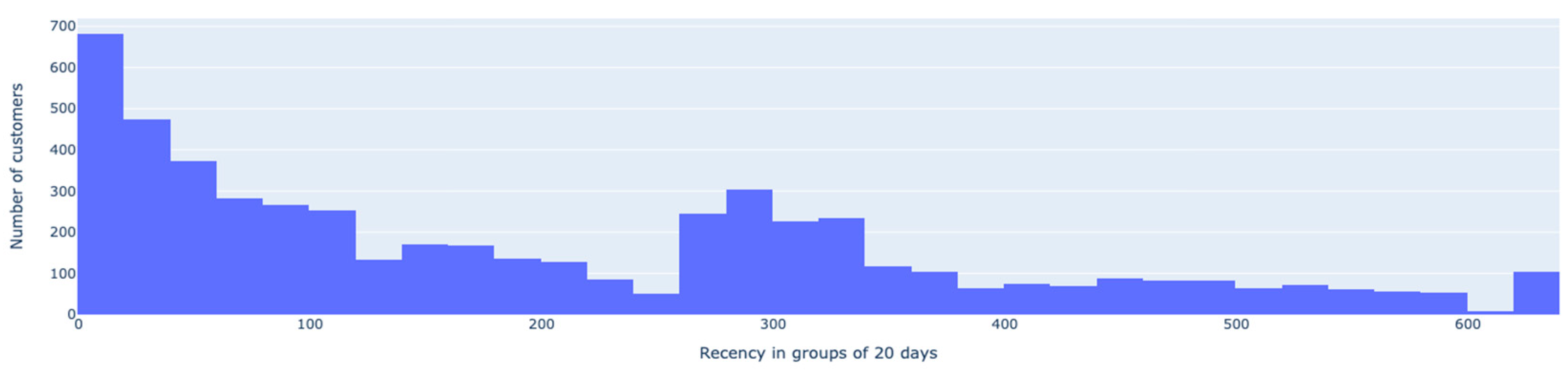
Before determining the NPD, the recency and frequency of each customer is calculated to have a better view of the dataset.

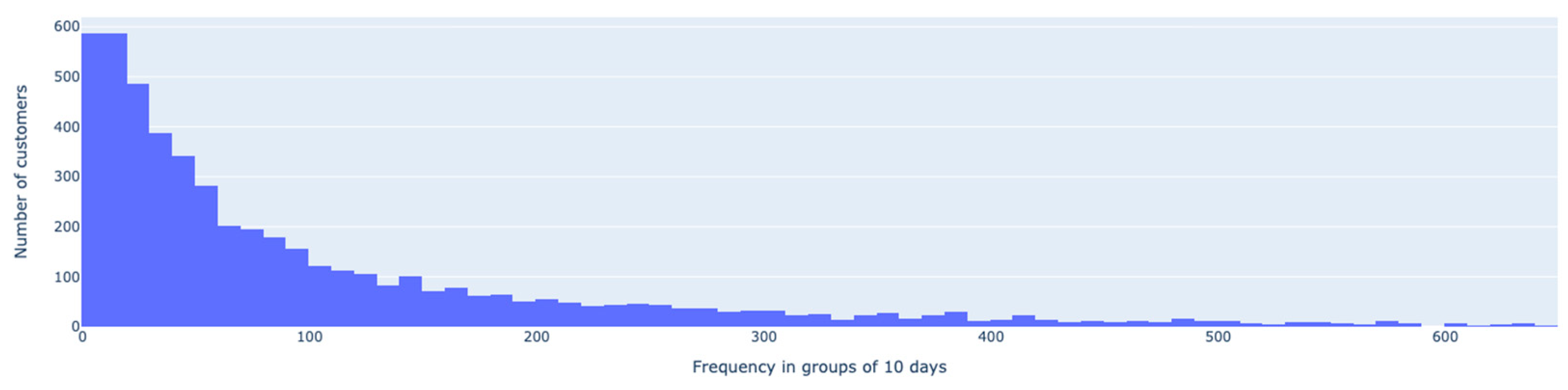
The customer recency determines how recently a customer made a purchase. In Figure 4, it can be noticed that there is a higher distribution of customers that made a new purchase in the first 20 days. The frequency is shown in Figure 5 and represents the number of times a customer makes a purchase. This is exemplified in Table 2 using the selected dataset. The higher number of orders, the more frequently a customer buys. This is important in filtering the customers that are the most relevant for determining the NPD. The proposed solution requires a significant amount of past data and works best with customers that already have a track record of purchases. To forecast x days into the future, a time series forecasting model usually requires at least 2x past days. In this study, 4x days have been selected to avoid bias related to customers with fewer orders. It forecasts the next 5 days, selecting 411 customers with at least 20 orders. For the other customers, this analysis is not relevant.

Figure 4. Customers’ recency distribution.

Figure 5. The frequency distribution of customers’ orders.

Table 2. The last NPD, recency, frequency, and cluster for the selected dataset.

	Customer ID	NPD	Recency	Frequency	Cluster
1	13085.0	9999.0	57	92	3
2	13078.0	13.0	0	855	3
3	18102.0	27.0	26	1068	3
4	12682.0	15.0	0	1042	3
5	18087.0	46.0	44	95	3

The elbow method is used to determine the optimal number of clusters for the input of the k-means algorithm. Figure 6 shows that the best number of clusters in our case is four, and Table 3 presents the descriptive statistics for each cluster. In this table, “Count” represents the number of values, “Mean” represents the average, “Std” represents the standard deviation, “Min” and “Max” are the minimum and maximum values, and “25%”, “50%” and “75%” represent the first, second, and third quartile. More specifically, when the instance values are arranged in increasing order, “x%” is the value under which x% of instance values are found.

Figure 6. The within clusters sum of squared errors (SSE) employed to select the most appropriate number of clusters using the elbow method.

Table 3. Descriptive statistics for the selected dataset of each cluster.

Cluster	Count	Mean	Std	Min	25%	50%	75%	Max
1	750	520.50	65.21	418	465	517	571.5	638
2	1427	314.36	41.12	236	281.5	308	338	416
3	1101	155.62	39.24	97	118	153	187	234
4	2037	37.96	27.74	0	13	33	59	96

The period between purchases is measured in days. Two examples for the customers with ids 14395 and 14911 can be seen in Figure 7 and Figure 8, respectively. The first is a customer with a smaller frequency, and the second is a customer with a higher frequency. These examples are considered to show how the models perform in these situations.

Figure 7. Time series data with the NPDs for customer 14395.

Figure 8. Time series data with next purchase days for customer 14911.

4.2. Models

The models selected for comparison with the proposed transformer model are ARIMA, XGBoost, and LSTM. The parameters for each model that offer the best results, according to the experiments performed, are shown in Table 4.

Table 4. Parameters used in experiments.

Algorithm	Parameters
ARIMA	automatically searches the parameters: number of lag observations, degree of differencing, order of the moving average
XGBoost	input length: 2 · forecast length loss: squared error estimators: 1000 learning rate: 0.3
LSTM	optimizer: Adam loss: mean squared error LSTM layers: 4 epochs: 300 batch size: 8
Transformer	optimizer: Adam epochs: 100 encoder layers: 128 attention layers: 128 attention heads: 8 dropout rate: 0.8 learning rate: 0.001

The ARIMA model is implemented using the AutoTS Python package [20] using only ARIMA models to determine the best combination for the selected dataset. XGBoost Python package [21] is used to implement the model using the XGBRegressor wrapper interface. The LSTM model is implemented in Tensorflow [22] using a sequential model with LSTM and dense layers. The transformer model is implemented in Tensorflow, and the Scikit-learn package is used for the k-means algorithm [23].

4.3. Results

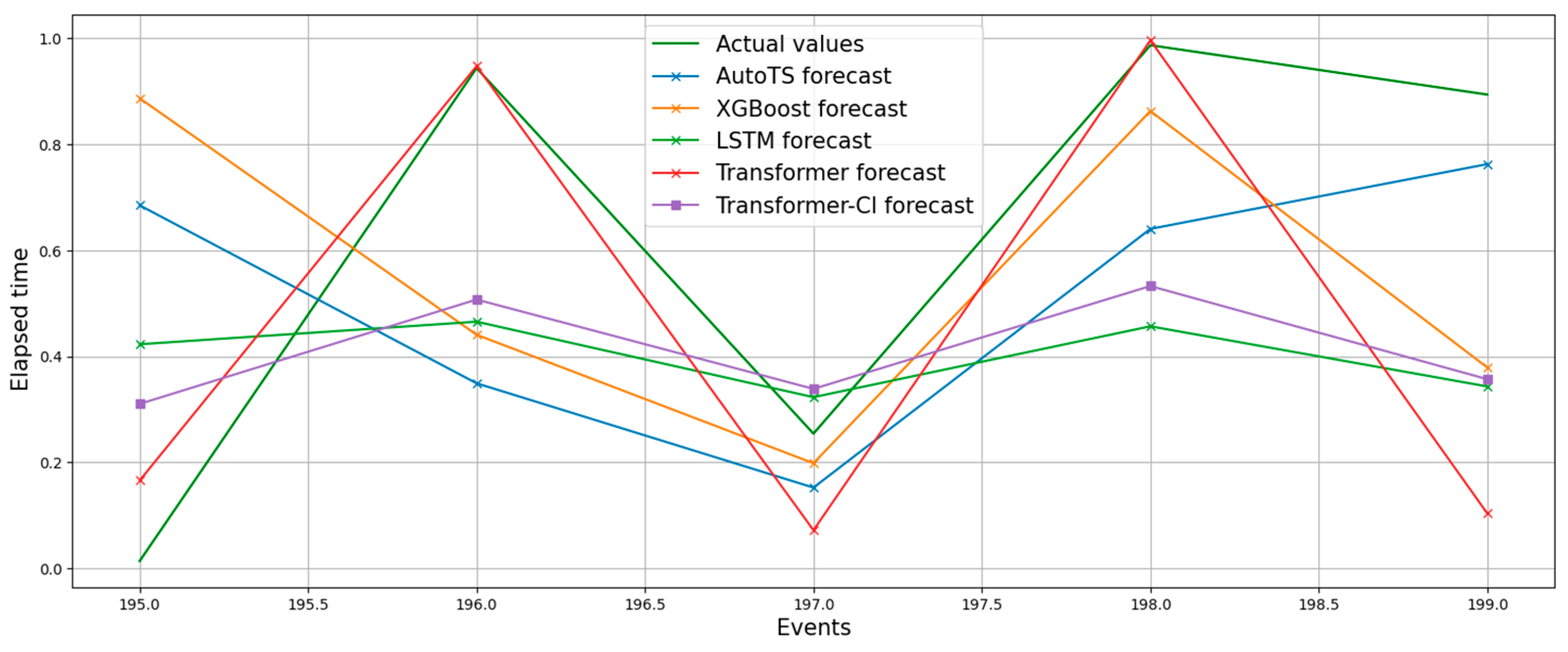
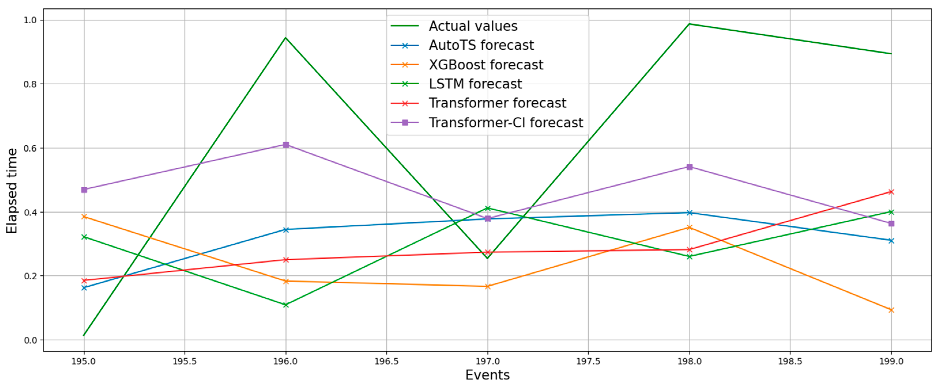
The experiments performed focus on predicting the next five purchase days to determine how likely a customer is to make new purchases. Two examples are used to show how the models perform on different time series. In Figure 9 (for the customer with id 14395), the models tend to fit the series better, especially the transformer, while in Figure 10, (customer with id 14911) the models tend to average the prediction values as the calculated predictions. RMSE and MAE are used to evaluate the performance of the models.

Figure 9. Time series using selected models for customer 14395.

Figure 10. Time series using selected models for customer 14911.

Performing an augmented Dickey–Fuller test [24] on these time series can determine whether the time series are stationary or not. The first one has a p-value of 0.733492, which means it is stationary, while the second one has a p-value of 0.000002, meaning it is not stationary. The stationarity of a time series means that its statistical properties such as mean, variance, and auto-covariance remain constant over time. A stationary time series is often easier to model and forecast. This can be one of the reasons why the models perform better on the stationary dataset, but there are also other factors that can influence the prediction such as data quality, randomness, or complexity.

The mean RMSE values for the two customers and the average values for each model are shown in Table 5. Analyzing the RMSE values on both examples, the differences between the models tend to remain similar, even though the mean RMSE is higher in the first one.

Table 5. Mean RMSE results using selected models for customers 14395 and 14911.

Customer	ARIMA	XGBoost	LSTM	Transformer	Transformer- Clustered
14395	0.4361	0.5096	0.5218	0.3767	0.3950
14911	0.3185	0.3203	0.3283	0.3159	0.3618
Average	0.3773	0.4149	0.4250	0.3463	0.3784

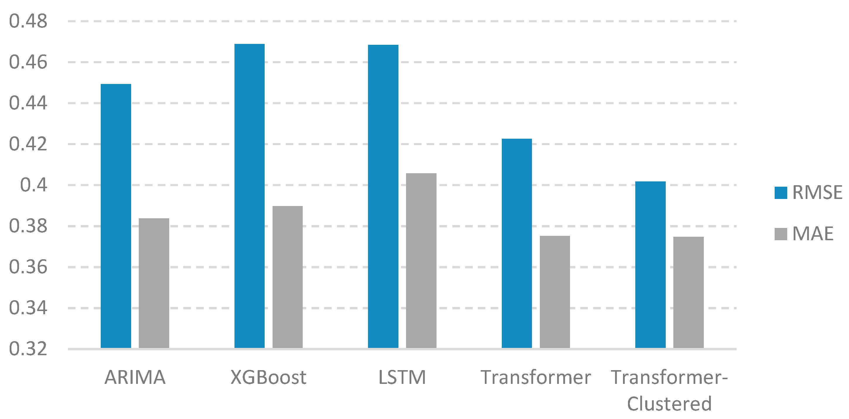
To determine the overall performance of the models, an experiment was executed for the 411 customers. Figure 11 shows a comparison of RMSE and MAE values for the selected models. The transformer model has a 6.15% improvement considering the RMSE and 2.25% improvement in MAE against the best classic model, ARIMA. The clustered transformer model has an 11.20% improvement in RMSE and 2.35% in MAE against the ARIMA model. The experiments show that the transformer-based forecasting is able to make good predictions for the problem under study.

Figure 11. The errors obtained by the selected models.

The execution speed is also reduced significantly by clustering the customers. This is demonstrated against other studies that focus on ARIMA, XGBoost, LSTM, and combination of these methods.

It can also be seen that linear models, such as ARIMA, perform well and are usually the first choice when considering a time series forecasting application. On this dataset, the advantage of the proposed transformer is its efficiency in capturing long-term dependencies within time series data through the self-attention mechanisms. Unlike ARIMA, transformers do not rely on assumptions of stationarity and can adapt to diverse time series patterns, including trends, seasonality, and irregularities. To improve ARIMA, external regressor variables, such as holidays, weekends or others, are used. In the scope of NPD, the external regressor cannot be used in the same way because the dataset does not take into account actual dates, but rather a series of data that does not have a direct real-world correspondence.

XGBoost usually offers fast and accurate results, which gives it a competitive advantage if execution time is the most important factor. When looking at the results, it is similar to ARIMA and does not fit the series properly. This is because it cannot deal with time series data containing long-term dependencies, seasonal patterns, or irregular trends as well as the proposed model. The transformer’s ability to handle long-range dependencies without manual feature engineering is very beneficial in this particular case.

Against the LSTM model, the transformer has an advantage in the execution speed. The transformer architecture is designed to be parallelized and to use the graphics processing unit (GPU). The parallel computation capability of transformers accelerates training and allows for the effective extraction of complex features, minimizing the need for manual feature engineering. This is important when scaling to a larger dataset. The scores also show a difference in this experiment. The attention mechanism enables the model to focus on the most important time steps and features, enhancing adaptability to changing patterns.

5. Conclusions

Today’s e-commerce stores are effective online platforms that give businesses access to a global consumer base, promote easy shopping experiences, and play an important part in modern commerce. Predicting the NPD of customers is an important metric that can help businesses understand and predict customer behavior, allowing for strategic planning and targeted marketing efforts to increase customer retention, enhance loyalty, and optimize sales and revenue in the long term.

While other studies on NPD prediction focus on known methods for time series forecasting, such as ARIMA, XGBoost and LSTM, this article proposes a new approach, based on the transformer model. The experiments were conducted on an online retail dataset, where a subset of customers were selected to determine their NPD. The proposed model was compared with the abovementioned techniques and shown to offer an improvement in RMSE of 6.15%. To further increase the model performance, the customers were grouped using the k-means clustering algorithm, demonstrating an additional improvement of 5.05% in RMSE, and a clear reduction in execution time. The advantages of using the transformer model are as follows: efficiently scaling on GPU because of parallelization, capturing long-term dependencies within time series data through self-attention mechanisms, and training the model on multiple time series by clustering to better capture the patterns in data. One of the limitations of the transformer model is that the self-attention mechanism is permutation-invariant and affects the order of the values returned, which impacts time series data more than in NLP applications.

The successful application of the transformer model in this context encourages further exploration and adoption of transformer-based solutions for a wide range of predictive analytics and forecasting tasks in the evolving e-commerce space. There are several paths to further expand the utilization of these models for predicting customers’ NPD in the e-commerce domain. Addressing the challenge of imbalanced data present in customer purchase data is an important step. Integration of external features, such as marketing campaigns, seasonal trends, and customer demographics into the model, can improve the predictive accuracy by accounting for a broader array of influences on customer behavior. The proposed model should also be applied to multiple public benchmark time series to demonstrate its generalizability. Another direction of research is to explore the ensemble methods that combine the strengths of various predictive models, which could offer a robust predictive framework. Continuous model retraining is also important when applying a model in production, as it needs to remain effective in a dynamic landscape of e-commerce stores that are continuously changing. Enhancing interpretability and researching new methods of efficient retraining is also important for optimal results.