A General Procedure to Formulate 3D Elements for Finite Element Applications

Abstract

This paper presents a general procedure to formulate and implement 3D elements of arbitrary order in meshes with multiple element types. This procedure includes obtaining shape functions and integration quadrature and establishing an approach for checking the generated element’s compatibility with adjacent elements’ surfaces. This procedure was implemented in Matlab, using its symbolic and graphics toolbox, and complied as a GUI interface named ShapeGen3D to provide finite element users with a tool to tailor elements according to their analysis needs. ShapeGen3D also outputs files with the element formulation needed to enable users to implement the generated elements in other programming languages or through user elements in commercial finite element software. Currently, finite element (FE) users are limited to employing element formulation available in the literature, commercial software, or existing element libraries. Thus, the developed procedure implemented in ShapeGen3D offers FEM users the possibility to employ elements beyond those readily available. The procedure was tested by generating the formulation for a brick element, a brick transition element, and higher-order hexahedron and tetrahedron elements that can be used in a spectral finite element analysis. The formulation obtained for the 20-node element was in perfect agreement with the formulation available in the literature. In addition, the results showed that the interpolation condition was met for all the generated elements, which provides confidence in the implementation of the process. Researchers and educators can use this procedure to efficiently develop and illustrate three-dimensional elements.

1. Introduction

The finite element method (FEM) is a popular numerical technique for solving partial differential equations (PDE) in engineering and mathematics. Traditional areas in which this method has been applied include structural analysis, heat transfer, fluid flow, mass transport, electromagnetic potential, and augmented reality [1,2,3,4,5]. Under this method, the domain is subdivided into smaller parts, called elements, composed of multiple nodes. The number of nodes within an element determines the order of the interpolation function that represents the approximate solution of the PDE. The interpolation function is defined in terms of nodal basis functions, also known as shape functions. The error associated with the interpolation is minimized using the calculus of variation, resulting in a system of algebraic equations. The variational formulation also requires the integration of finite element variables that are a function of shape functions and other properties, such as shape function derivatives, over the element’s domain. These integrals are approximated using a quadrature rule, which requires selecting appropriate integration points and corresponding weights to obtain an exact integration. Finally, each element’s equations are combined into a larger system of equations that models the entire problem.

The shape functions and integration quadrature are essential parts of the FEM formulation of an element. Generally, the nodal shape functions are defined in a reference element in local coordinates. If the same shape functions used to interpolate displacements in a reference element are used to map local and global coordinates, they are termed isoparametric elements. The nodal functions and integration quadrature are available for several three-dimensional elements in the literature and are incorporated into commercial FEM software. These elements are generally lower order and limited to four specific elements: hexahedrons from the Lagrangian and Serendipity families, tetrahedrons, prisms, and pyramids [6]. For instance, ABAQUS [7] only offers elements of quadratic order to model solids, including a hexahedron from the Serendipity family, also known as the 20-node brick element, tetrahedrons, and prism elements.

Researchers generally use elements only up to the second order of the geometries mentioned above when modeling three-dimensional solids. However, there is a need to employ elements of higher order in many applications. For instance, transition elements are extensively used for mesh refinement [8], where relying only on quadratic elements brings up hanging node problems. Unconventional elements, such as the xNy-element concept [9], are developed to tackle this issue. Transition elements are also employed in contact problems. Buczkowski [10] developed 22 and 21-node elements, and Smith et al. [11] developed 14-node hexahedral isoparametric elements to analyze contact problems by modifying the 8 and 20-node hexahedral elements. In addition to transition elements, there is also a need for higher-order three-dimensional elements as they offer higher accuracy in calculating Lagrangian solid dynamics. For instance, the spectral finite element method [12] uses the interpolation function of high-order Lagrange polynomials to capture high-frequency wave propagation that benefits fields such as structural health monitoring [13,14,15,16] and seismology [17].

Formulating shape functions for elements with arbitrary numbers of nodes in 3D requires defining the nodal distribution, interpolation functions, and integration quadrature. The method for determining the shape functions [3] requires incorporating a polynomial function as the interpolation function in each nodal point. These calculations can be carried out by hand for one-dimensional and lower-order two-dimensional elements. For three-dimensional cases, the procedure is extremely laborious. Another aspect in generating the element formulation is verifying that the shape functions fulfill the following conditions [3]: (a) Interpolation: take a unit value at node $\mathit{i}$ and zero at all other nodes; (b) Local support: vanish over any element boundary that does not include node $\mathit{i}$; and (c) Interelement compatibility: No discontinuities at the element boundary, i.e., for solid mechanics applications, the elements should deform along the common surface without openings and overlaps. If two elements share a surface, the difference in the value of the shape functions at common nodal points between the two elements should be zero. If the element is a hexahedron or tetrahedron, the need to define the nodal distribution can be avoided by following specific procedures available in the literature. For the hexahedron element of the Lagrangian family, the procedure is explained in [3], whereas in the case of the Serendipity family, Arnold and Arnold [18] provided the theory to obtain shape functions for any given order. In the case of higher-order tetrahedrons, Silvester [19] proposed a simple and elegant procedure based on four-digit node numbering to obtain nodal coordinates that generate a uniform nodal distribution, which is observed to cause Runge oscillations [20]. Some alternative nodal distributions to mitigate this effect are Fekete points, Gauss–Legendre points, and Chebyshev points.

There are several methods to obtain the integration quadrature, such as the Gaussian quadrature rule [21] and Legendre–Gauss–Lobatto nodes [22] for hexahedrons. In the case of higher-order tetrahedrons, the standard collapsed coordinate system that maps the quadrature to the tetrahedron from a reference hexahedron [23] is a popular choice. Another approach is based on the integration scheme used for the finite cell method, where a high-order tetrahedron is subdivided into multiple sub-tetrahedrons [20], and numerical integration is carried out on each of them using Gaussian quadrature.

Several existing libraries provide the nodal shapes for higher-order elements that have been obtained a priori. For example, ELEMENTS [24] is a library written in c++ that focuses on supporting novel element spaces, such as Serendipity element space and any order spectral elements. Nekter++ [25] is a FEM solver that supports variable polynomial order in space and heterogeneous polynomial order within two and three-dimensional elements. Scilab [26] is another platform that offers spectral elements in 2D. Some other libraries, such as deal.ii [27], Dune [28], and MFEM [29] are also available. These codes do not generate shape functions nor determine the appropriate integration quadrature for a custom element and do not provide a visual representation.

No methodology exists in the literature for formulating elements of arbitrary order in an automated way. Moreover, if a new element is generated, checks must be performed to guarantee that the interpolation and location support conditions are satisfied. Such a task is difficult to perform for a 3D element as they contain more than three boundaries or surfaces where the local support condition needs to be satisfied for each shape function. In addition, an approach must be established to verify the interelement compatibility of elements in a multielement mesh. Hence, a general procedure is developed in this paper to perform these tasks programmatically. This procedure is capable of generating shape functions and integration quadrature for: (1) arbitrary or custom elements with a given nodal distribution and interpolation function; (2) hexahedrons of the Serendipity and Lagrange families; and (3) tetrahedrons of any given element order. The integration quadrature includes integration points and weights for: (1) volume; and (2) surface integration. The normal vector and parametric coordinates for each element surface are also obtained to enable users to implement the traction vector in FEM applications. The interpolation and local support conditions are checked qualitatively through computer graphics, while interelement compatibility is verified by establishing expressions that ensure nodal shape agreement from adjacent elements at common nodes.

An attractive feature of the proposed procedure is that it can be automated using symbolic and graphical tools, readily available in programming platforms such as Matlab, Python, and Mathematica. In this paper, Matlab was used to implement the procedure, but other users can program the procedure on the platform of their choice. In addition, a Graphical User Interfaces (GUI), named ShapeGen3D (ShapeGen 3D installation file link: https://github.com/sjdyke-reth-institute/ShapeGen3D/blob/main/ShapeGen3D.mlappinstall, accessed on 19 September 2023), was developed to expedite the use of the procedure. GUIs have facilitated the implementation of novel techniques developed by FE code developers, such as in [30,31]. Hence, the development of ShapeGen3D can serve as an interactive approach for developing 3D elements and providing finite element users the flexibility to adopt elements of arbitrary order in their simulations.

The remainder of this paper is organized as follows. Section 2 presents the generalized procedure for generating element properties and explains the implementation of the GUI interface, ShapeGen3D. Section 3 obtains the formulation for several 3D elements through the use of ShapeGen3D. The numerical examples are relevant to applications that can be potentially impacted by this work, including the generation of tailored elements designed to reduce the computational cost associated with the analysis (Section 3.3), transition elements that connect fine to coarse mesh regions, such as in contact problems (Section 3.4), and high-order spectral elements to simulate wave propagation behavior (Section 3.5). Section 4 discusses the potential impact of this development in the computational mechanics field. Finally, Section 5 concludes with some final remarks.

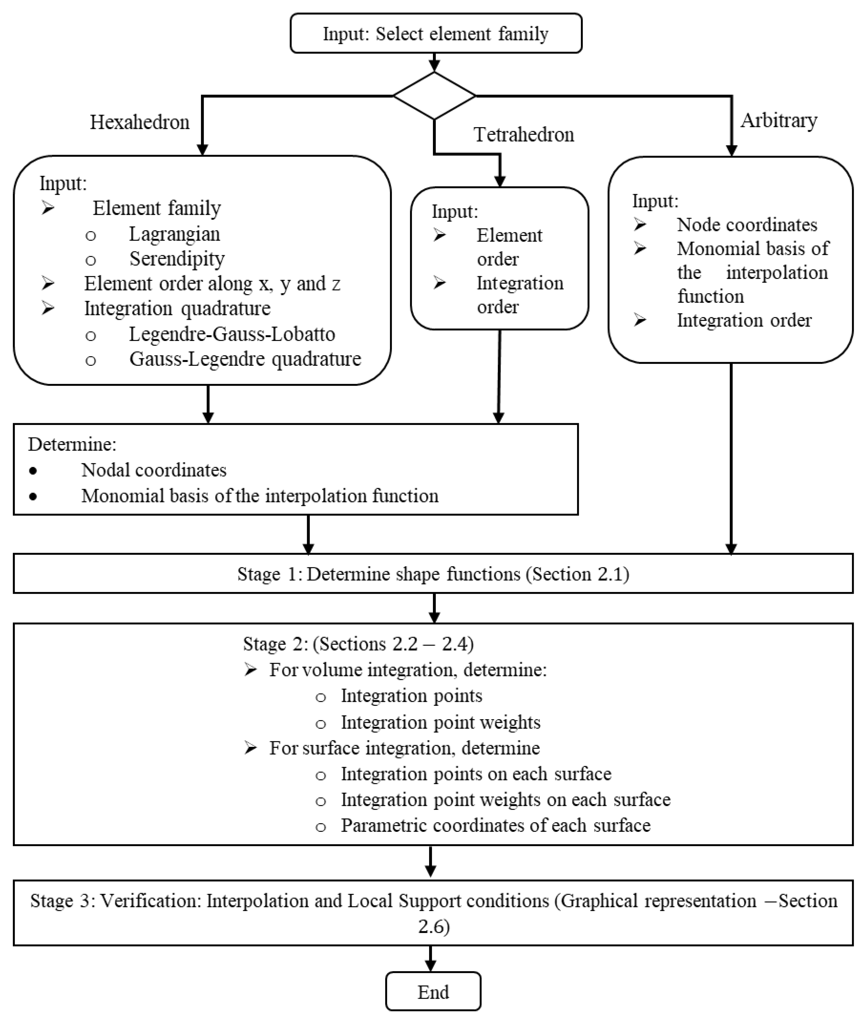
2. Materials and Methods

This section illustrates the general procedure to formulate and implement an element within a multielement FE mesh through computer implementation. The formulation of the element includes three stages, which are (1) the generation of shape functions, (2) integration quadrature, and (3) verification by checking interpolation and local support conditions. If stages 1 and 2 are completed, the element can be incorporated into a multielement mesh if the interelement compatibility is satisfied between the adjacent elements of different types. Hence, stage 3 checks the elements’ compatibility. The procedure was outlined in such a way as to make computer implementation possible. This procedure was implemented using a Matlab app with a GUI interface.

Figure 1 breaks down the steps to formulate an element (stages 1 to 3). At the input step, a distinction is made between hexahedron and tetrahedron elements and arbitrary elements. Arbitrary elements, such as transition elements, do not have any specified nodal coordinates and shape functions. Hence, an approach was developed that utilizes (1) nodal coordinates and (2) the monomial basis of the interpolation function to calculate the shape functions, as described in Section 2.1. The procedure for determining the shape functions of hexahedrons and tetrahedrons of elements followed existing literature (see Section 2.3 and Section 2.4).

Next, in stage 2, the volume and surface integration quadrature are obtained. The integration quadrature in volumetric space includes only integration points and weights, whereas the surface integration quadrature includes integration points, weights, and parametric coordinates for each element’s surface. As arbitrary elements do not have any reference quadrature, a method similar to the finite cell method [32,33] was implemented, as described in Section 2.2. Following this approach, the integration quadrature for any element type can be determined for both volume and surface integrations in an automated way, allowing computer implementation. Moreover, the formulation of standard quadratures for hexahedrons and tetrahedrons was implemented as outlined in Section 2.3 and Section 2.4, respectively. Stage 3 is a verification step to check the interpolation and local support conditions. This verification was conducted through a graphical representation of the shape function in Matlab (see Section 2.6). The locations where the shape functions yield a 0 value are presented as a void (blank space).

For the final implementation stage, if an element is to be incorporated into a multielement mesh, the interelement compatibility condition between two adjacent elements must be checked. In this paper, a method was developed that can be used to check this condition for each of the integration points of the adjacent surfaces numerically. Such a task is highly labor-intensive to perform by hand for 3D elements, but it can be automized, as presented in Section 2.5. Figure 2 shows the overview of this stage, which requires the input of the surface pairs that will form the interelement boundary.

The layout of this methodology was essential for developing GUI software that automizes the generation of arbitrary 3D element formulation. Finally, Section 2.7 shows the implementation of the GUI interface, which facilitates the execution of the procedure outlined in Figure 1 and Figure 2.

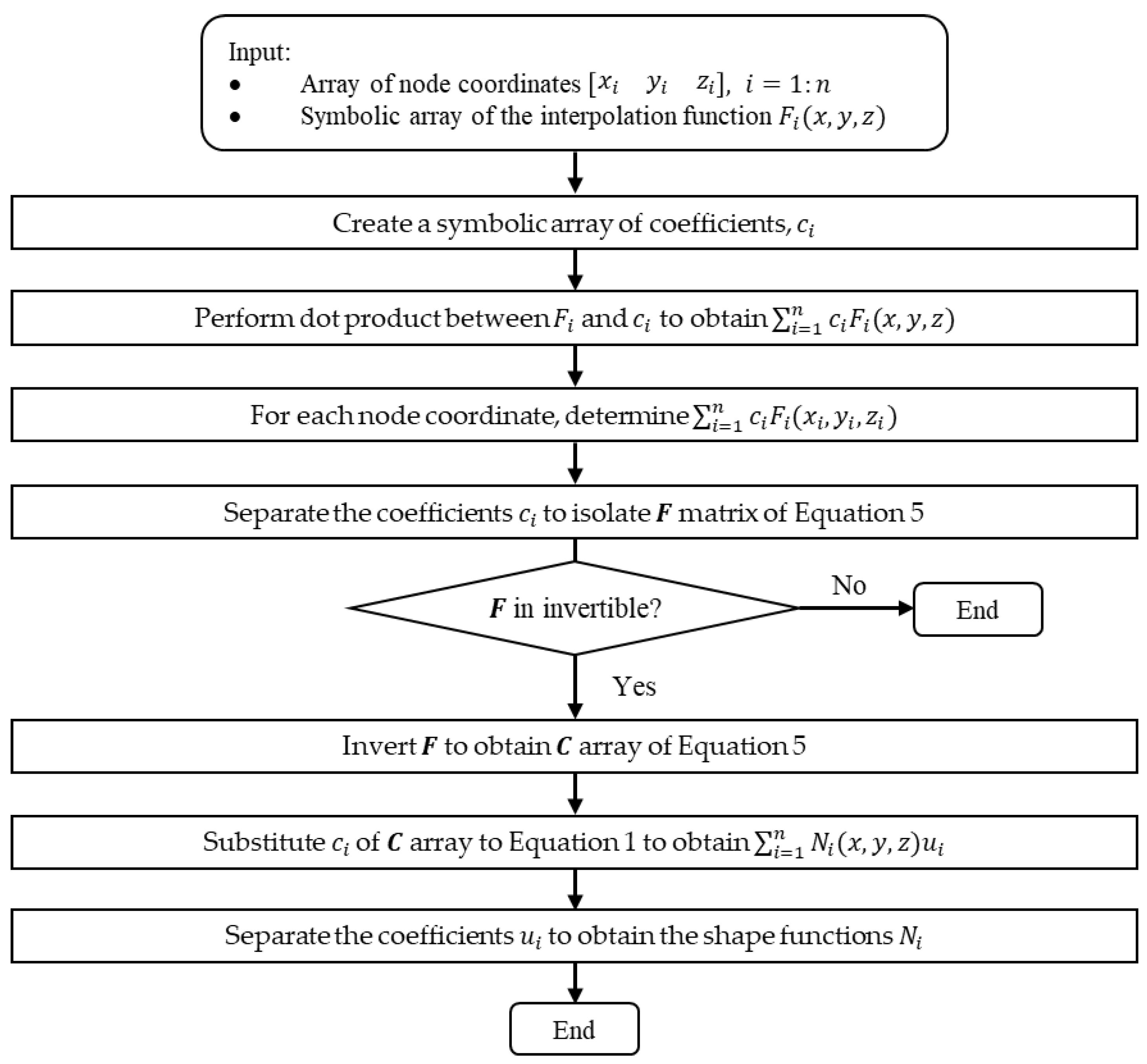
2.1. Computation of Shape Functions for a Given Nodal Distribution and Interpolation Function

The generation of shape functions of the development stage is discussed here. Assume that an element defined by a node-set ${\mathit{P}}_i=\left[\begin{array}{ccc}{x}_i& y_i& z_i\end{array}\right]$ consists of $n$ nodes and an interpolation function $f_n\left(x,y,z\right)$. If $f_n\left(x,y,z\right)$ is a linear combination of arbitrary constants $c_i$ and a function with a monomial basis, $F_i(x,y,z)$, then the interpolation function can be written as

$$f_n\left(x,y,z\right)=\sum _{i=1}^n{c}_i{F}_i(x,y,z)$$

(1)

This function, $f_n$, can also be expressed in terms of the shape function terms, $N_i$, as

$$f_n\left(x,y,z\right)=\sum _{i=1}^n{N}_i(x,y,z)u_i$$

(2)

where $u_i$ is a variable associated with node $i$. Plugging Equation (1) into Equation (2)

$$\sum _{i=1}^n{c}_i{F}_i(x,y,z)=\sum _{i=1}^n{N}_i(x,y,z)u_i$$

(3)

The shape functions can be obtained for a given set of known function ${\mathit{F}}_{\mathit{i}}$ by manipulating Equation (3) to solve for parameters ${\mathit{c}}_{\mathit{i}}$. In matrix form, this operation becomes x

$$\left[\begin{array}{c}{c}_1\\ c_2\\ .\\ .\\ c_n\end{array}\right]={\left[\begin{array}{ccccc}{F}_1\left({\mathit{P}}_1\right)& F_2\left({\mathit{P}}_1\right)& .& .& F_n\left({\mathit{P}}_1\right)\\ F_1\left({\mathit{P}}_2\right)& F_2\left({\mathit{P}}_2\right)& .& .& F_n\left({\mathit{P}}_2\right)\\ .& .& .& .& .\\ .& .& .& .& .\\ F_1\left({\mathit{P}}_n\right)& F_2\left({\mathit{P}}_n\right)& .& .& F_n\left({\mathit{P}}_n\right)\end{array}\right]}^{-1}\left[\begin{array}{c}{u}_1\\ u_2\\ .\\ .\\ u_n\end{array}\right]$$

(4)

$$\mathit{C}={\mathit{F}}^{-1}\mathit{U}$$

(5)

Plugging $c_i$ in Equation (3) and isolating $u_i$, yields the shape functions [4]. If the interpolation function $f_n$ is unable to form a non-invertible matrix $\mathit{F}$ with node set $\mathit{P}$, then the node-set and interpolation function are not valid. If invertible, shape functions can be formulated that automatically satisfy the interpolation and partition of unity condition. This method cannot be used to generate shape functions for rational polynomials, such as in the case of Wachspress basis functions [34] and Radial basis functions [35]. This approach for determining shape functions was implemented using the symbolic toolbox in Matlab. The steps implemented in the Matlab routines are summarized in Figure 3.

2.2. Determination of Integration Quadrature for an Arbitrary Element

The integration quadrature for an arbitrary element is determined following an approach similar to the finite cell method [32,33], which involves dividing the element into a finite number of tetrahedron cells and mapping the integration points from a reference tetrahedron to each cell. First, the Delaunay triangulation [36] is carried out for the given set of node $\mathit{P}$, which subdivides the arbitrary element into multiple tetrahedrons in the $xyz$ space. Each of the tetrahedrons is termed as $S_e$, where the subscript $e$ indicates the element number with nodal coordinates $(x_n,y_n,z_n)$, and $n$ can take values from 1 to 4. Next, a reference element, consisting of a standard orthogonal tetrahedron in $\xi \eta \gamma$ space with vertices $\left(0,0,0\right),\left(1,0,0\right),$ $(0,1,0)$, and $(0,0,1)$ is formulated. An integration quadrature, i.e., integration points and weights, up to order 4 is used from [37] for such reference tetrahedron element. The shape functions of the reference 4-noded tetrahedron element are

$$\begin{gathered} N_1=1-\xi -\eta -\gamma \\ {N}_2=\xi \\ {N}_3=\eta \\ {N}_4=\gamma \end{gathered}$$

(6)

Finally, the integration quadrature of the global cells or tetrahedrons is calculated. Each integration point coordinate $({\xi }_i,{\eta }_i,{\gamma }_i)$ from the reference tetrahedron in $\xi \eta \gamma$ space is mapped to each $S_e$ in the $xyz$ space following Equation (7) [3]

$$\left[\begin{array}{c}x\\ y\\ z\end{array}\right]={\left[\begin{array}{cccccccccccc}{N}_1& 0& 0& N_2& 0& 0& N_3& 0& 0& N_4& 0& 0\\ 0& N_1& 0& 0& N_2& 0& 0& N_3& 0& 0& N_4& 0\\ 0& 0& N_1& 0& 0& N_2& 0& 0& N_3& 0& 0& N_4\end{array}\right]}_{{\xi }_i,{\eta }_i,{\gamma }_i}\left[\begin{array}{c}{x}_1\\ y_1\\ z_1\\ .\\ .\\ x_4\\ y_4\\ z_4\end{array}\right]$$

(7)

The weight of the integration points for the global element $\left(w_i^{\mathit{x}}\right)$, where superscript $\mathit{x}$ indicates $xyz$ space, is mapped by multiplying the weights of integration points of the reference element $\left(w_i^{\mathit{\xi }}\right)$ with the determinant of Jacobian, as $w_i^x=\left|\mathit{J}\right|w_i^{\mathit{\xi }}$. Following the isoparametric mapping, the Jacobian matrix can be determined as

$$\mathit{J}=\left[\begin{array}{ccc}\frac{\partial x}{\partial \xi }& \frac{\partial y}{\partial \xi }& \frac{\partial z}{\partial \xi }\\ \frac{\partial x}{\partial \eta }& \frac{\partial y}{\partial \eta }& \frac{\partial z}{\partial \eta }\\ \frac{\partial x}{\partial \gamma }& \frac{\partial y}{\partial \gamma }& \frac{\partial z}{\partial \gamma }\end{array}\right]={\left[\begin{array}{cccc}\frac{\partial N_1}{\partial \xi }& \frac{\partial N_2}{\partial \xi }& \frac{\partial N_3}{\partial \xi }& \frac{\partial N_4}{\partial \xi }\\ \frac{\partial N_1}{\partial \eta }& \frac{\partial N_2}{\partial \eta }& \frac{\partial N_3}{\partial \eta }& \frac{\partial N_4}{\partial \eta }\\ \frac{\partial N_1}{\partial \gamma }& \frac{\partial N_2}{\partial \gamma }& \frac{\partial N_3}{\partial \gamma }& \frac{\partial N_4}{\partial \gamma }\end{array}\right]}_{{\xi }_i,{\eta }_i,{\gamma }_i}\left[\begin{array}{ccc}{x}_1& y_1& z_1\\ x_2& y_2& z_2\\ x_3& y_3& z_3\\ x_4& y_4& z_4\end{array}\right]$$

(8)

For linear tetrahedrons, i.e., the reference element,

$$\mathit{J}=\left[\begin{array}{cccc}-1& 1& 0& 0\\ -1& 0& 1& 0\\ -1& 0& 0& 1\end{array}\right]\left[\begin{array}{ccc}{x}_1& y_1& z_1\\ x_2& y_2& z_2\\ x_3& y_3& z_3\\ x_4& y_4& z_4\end{array}\right]$$

(9)

The integration quadrature on each surface is also determined to allow the computation of equivalent nodal flux. First, the surfaces of an element must be identified. This step can be accomplished by determining the convex hull [36], which is the smallest convex set that bounds all the nodes of an element. Hence, the convex hull of the Delaunay triangulation is determined to obtain the integration points and weights at the surfaces. Each surface $\mathit{s}$ of the set is a triangle with three vertices $(a_n,b_n,c_n)$, where $n$ is from 1 to 3. The integration point coordinates for a surface $\mathit{s}$ are determined as,

$${\mathit{x}}_s=\left[\begin{array}{c}x\\ y\\ z\end{array}\right]=\frac{1}{3}\left[\begin{array}{c}{a}_1+a_2+a_3\\ b_1+b_2+b_3\\ c_1+c_2+c_3\end{array}\right]$$

(10)

The normal vector for the surface, pointing outside the element interior, can be determined by performing the following cross-product operation as,

$${{}_s\mathit{n}}_z=\frac{\left(\left(a_2,b_2,c_2\right)-\left(a_1,b_1,c_1\right)\right)\times \left(\left(a_3,b_3,c_3\right)-\left(a_1,b_1,c_1\right)\right)}{‖\left(\left(a_2,b_2,c_2\right)-\left(a_1,b_1,c_1\right)\right)\times \left(\left(a_3,b_3,c_3\right)-\left(a_1,b_1,c_1\right)\right)‖}$$

(11)

where $‖\mathit{v}‖$ indicates the second norm of vector $\mathit{v}$. The parametric coordinates of a surface $s$, ${{}_{\mathit{s}}\mathit{n}}_{\mathit{x}},{{}_{\mathit{s}}\mathit{n}}_{\mathit{y}}$ can be determined as

$${{}_s\mathit{n}}_y=\frac{\left(\left[\begin{array}{ccc}{b}_1& b_2& b_3\end{array}\right]-\left[\begin{array}{ccc}{a}_1& a_2& a_3\end{array}\right]\right)}{‖\left[\begin{array}{ccc}{b}_1& b_2& b_3\end{array}\right]-\left[\begin{array}{ccc}{a}_1& a_2& a_3\end{array}\right]‖}$$

(12)

$${{}_s\mathit{n}}_x={{}_s\mathit{n}}_z\times {{}_s\mathit{n}}_y$$

(13)

The area of the surface is the weight of the integration, which can be determined as

$$w_s=\frac{1}{2}\left|n\right|$$

(14)

2.3. Formulation of Nodal Coordinates and Integration Quadrature for Hexahedron Elements

A standard orthogonal hexahedron in $xyz$ space is considered to formulate hexahedron elements with eight vertices as $\left(1,-1,-1\right)$, $\left(1,1,-1\right)$, $\left(-1,1,-1\right)$, $\left(-1,-\mathrm{1,1}\right)$, $\left(1,-1,1\right)$,$\left(1,1,1\right)$, $(-1,1,1)$. If $c_n$ is an arbitrary constant, the interpolation function for Lagrange family elements can be written as,

$$f_n=\sum _{i=0,j=0,k=0}^{i=m_x,j=m_y,k=m_z}{c}_n{x}^i{y}^j{z}^k$$

(15)

where $m_x,m_y$, and $m_z$ are the polynomial order along $x,y,$ and $z$ axis. For the Serendipity family, the interpolation function for such element can be obtained as,

$$f_n=1+\sum _{i=1,j=0,k=0}^{i=m_x,j=1,k=1}{c}_n{x}^i{y}^j{z}^k+\sum _{i=0,j=1,k=0}^{i=1,j=m_y,k=1}{c}_n{x}^i{y}^j{z}^k+\sum _{i=0,j=0,k=1}^{i=1,j=1,k=m_z}{c}_n{x}^i{y}^j{z}^k$$

(16)

Many studies and codes [37,38] follow a uniform nodal distribution that exhibits Runge oscillations. To avoid this numerical artifact, this development follows Legendre–Gauss–Lobatto nodes [22] where the node coordinates for each of the three axes, ${}_x\mathit{P},{}_y\mathit{P},{}_z\mathit{P}$, is the solution of Equations (17)–(19) between $+1$ and $-1$, respectively.

$$\left(1-x^2\right)\frac{d}{dx}{L}_{m_x}\left(x\right)=0$$

(17)

$$\left(1-y^2\right)\frac{d}{dy}{L}_{m_y}\left(y\right)=0$$

(18)

$$\left(1-z^2\right)\frac{d}{dz}{L}_{m_z}\left(z\right)=0$$

(19)

where, $L_{m_x}$ indicates the Legendre polynomial of the degree $m_x$. Each of these vectors of Equations (17)–(19) comprise a set of $(m_x+1)$, $\left(m_y+1\right),$ and $(m_z+1)$, respectively. To obtain the nodal coordinates in three dimensions, a mesh grid of size $\left(m_y+1\right)\times \left(m_x+1\right)\times \left(m_z+1\right)$ is generated using the obtained one-dimensional grids. For the Lagrange family, all the mesh grid points were considered, whereas only the points on the element edges were considered for the Serendipity family elements.

For integration quadrature, Legendre–Gauss–Lobatto quadrature and Gauss–Legendre quadrature were computed for a given element order along the x, y, and z-axis. Similar to node generation, one-dimensional reference grids were generated at first. For the Legendre–Gauss–Lobatto quadrature [22], the weights ${}_x\mathit{w}$, for each component of a one-dimensional reference grid in the $x$ axis can be determined as

$$w_{x_i}=\frac{2}{m_x\left(m_x+1\right){\left(L_{m_x}\left(x\right)\right)}^2}$$

(20)

For the Gauss–Legendre quadrature [21], the coordinate of integration points in one dimension, ${}_{Ix}\mathit{P}$ can be determined as the solutions of Equation (21) between $+1$ and $-1$ as

$$L_{m_x}\left(x\right)=0$$

(21)

The corresponding weight components of ${}_x\mathit{w}$ can be determined as

$${}_x{w}_i=\frac{2}{(1-{{}_{Ix}\mathit{P}}_i^2){\left[{\left.\left(\frac{d}{dx}{L}_{m_x}\left(x\right)\right)\right|}_{{{}_{Ix}\mathit{P}}_i}\right]}^2}$$

(22)

Considering that ${}_{y}w$ and ${}_{z}w$ are reference grids for the weights along $y$ and $z$ axes, the weights $\mathit{w}$ for the integration points in 3D can be determined using the tensor product [39] as presented in Equation (23). The components of the product $\mathit{w}$ are then assigned to the corresponding points.

$$\mathit{w}={}_z\mathit{w}\ast \left({}_x\mathit{w}{}_y{\mathit{w}}^T\right)$$

(23)

where “$\ast$” indicates elementwise multiplication. For the surfaces, the interpolation order for each surface is determined before computing the integration quadrature. If a surface $s$ contains node $i$, the number of differentiations along each axis of the shape function that produces a constant can be set as the interpolation order. This operation can be performed for all the nodes contained by $s$, where the maximum order is chosen for the surface. For ${{}_{s}m}_x$, this condition can be defined using a constant $C$ as presented in Equation (24), which is carried out using the symbolic toolbox of Matlab.

$$\frac{{\partial }^n{N}_i}{\partial x^n}=C,{{}_{s}m}_x=\max (nforalli\in s)$$

(24)

The coordinates and weights of the integration points and parametric coordinates for each of the six surfaces for hexahedron elements, $x=1,x=-1,y=1,y=-1,z=1,\mathrm{and}z=-1$ are defined according to

Table 1. Integration points weights and parametric coordinates of the element’s surfaces.

Surface	Integration Point Weights	${{}_{\mathit{s}}\mathit{n}}_{\mathit{x}}^{\mathit{T}}$	${{}_{\mathit{s}}\mathit{n}}_{\mathit{y}}^{\mathit{T}}$	${{}_{\mathit{s}}\mathit{n}}_{\mathit{z}}^{\mathit{T}}$
$x=1$	${}_y\mathit{w}{{}_z\mathit{w}}^T$	$\left[\begin{array}{ccc}0& 1& 0\end{array}\right]$	$\left[\begin{array}{ccc}0& 0& 1\end{array}\right]$	$\left[\begin{array}{ccc}1& 0& 0\end{array}\right]$
$x=-1$	${}_y\mathit{w}{{}_z\mathit{w}}^T$	$\left[\begin{array}{ccc}0& 0& 1\end{array}\right]$	$\left[\begin{array}{ccc}0& 1& 0\end{array}\right]$	$\left[\begin{array}{ccc}-1& 0& 0\end{array}\right]$
$y=1$	${}_x\mathit{w}{{}_z\mathit{w}}^T$	$\left[\begin{array}{ccc}0& 0& 1\end{array}\right]$	$\left[\begin{array}{ccc}1& 0& 0\end{array}\right]$	$\left[\begin{array}{ccc}0& 1& 0\end{array}\right]$
$y=-1$	${}_x\mathit{w}{{}_z\mathit{w}}^T$	$\left[\begin{array}{ccc}1& 0& 0\end{array}\right]$	$\left[\begin{array}{ccc}1& 0& 0\end{array}\right]$	$\left[\begin{array}{ccc}0& -1& 0\end{array}\right]$
$z=1$	${}_x\mathit{w}{{}_y\mathit{w}}^T$	$\left[\begin{array}{ccc}1& 0& 0\end{array}\right]$	$\left[\begin{array}{ccc}0& 1& 0\end{array}\right]$	$\left[\begin{array}{ccc}0& 0& 1\end{array}\right]$
$z=-1$	${}_x\mathit{w}{{}_y\mathit{w}}^T$	$\left[\begin{array}{ccc}0& 1& 0\end{array}\right]$	$\left[\begin{array}{ccc}1& 0& 1\end{array}\right]$	$\left[\begin{array}{ccc}0& 0& -1\end{array}\right]$

.

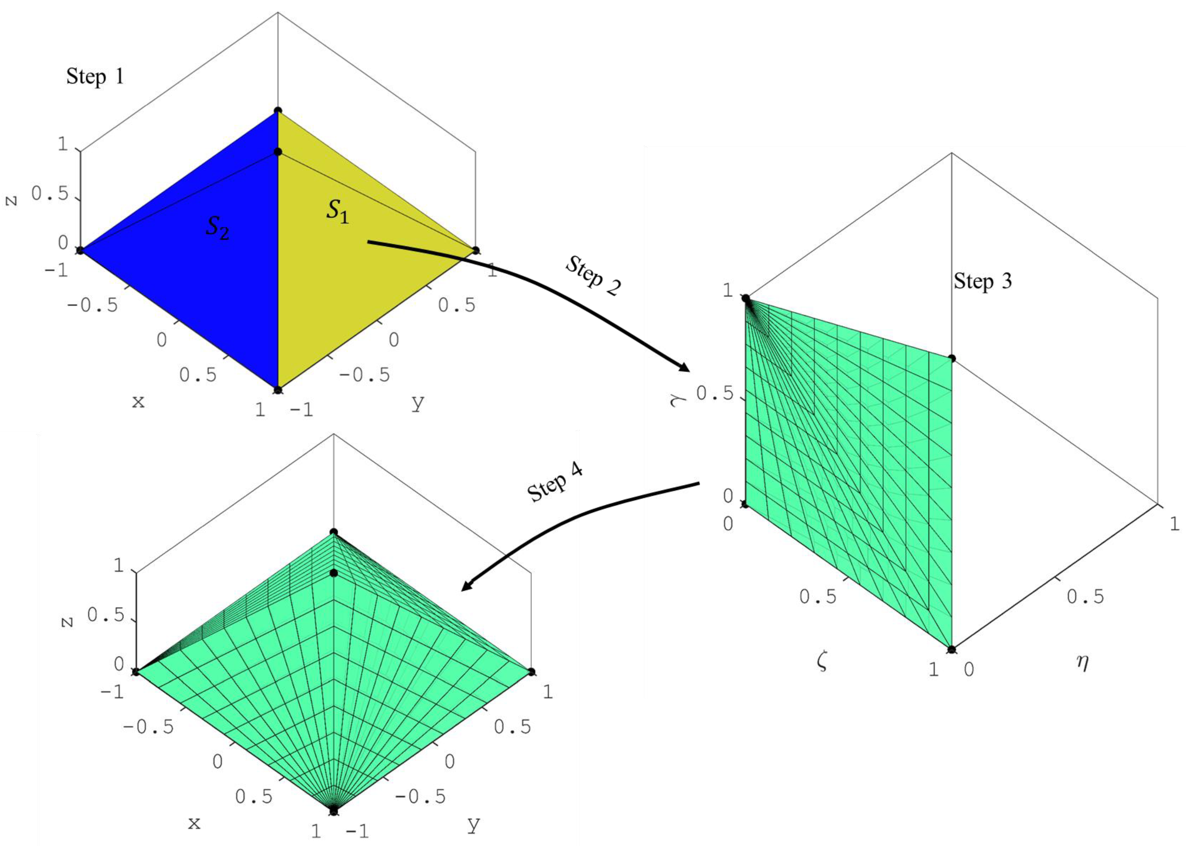
2.4. Formulation of Nodal Coordinates and Integration Quadrature for Tetrahedron Elements

This section presents the methodology implemented in the general procedure to formulate tetrahedron elements. The Lobatto triangle grid for orthogonal polynomials proposed by Luo et al. [40] is implemented to generate element properties for the standard orthogonal tetrahedron in $xyz$ space, which consists of four vertices as $\left(0,0,0\right),\left(1,0,0\right),$ $(0,1,0)$, and $(0,0,1)$. This nodal distribution does not exhibit Runge oscillations. According to this method, if an $m^{th}$ degree interpolating polynomial is used, the interpolation function can be expressed as,

$$f_n=\sum _{i=0,j=0,k=0}^{i=m,j=m,k=m}{c}_n{x}^i{y}^j{z}^{k}where,(i+j+k)\le m$$

(25)

where $c_n$ is an arbitrary constant. A one-dimensional reference grid comprising a set of $m-1$ degrees is generated as,

$$\mathit{v}=\frac{1}{2}(1+{}_x\mathit{P})$$

(26)

where ${}_x\mathit{P}$ is the solution of Equation (26) between the range +1 and −1 as,

$$\left(1-x^2\right)\frac{d}{dx}{L}_m\left(x\right)=0$$

(27)

The $L_m$ is the Legendre polynomial, which can be written as,

$$L_m\left(x\right)=\frac{1}{2^n}\sum _{k=0}^m\left(\begin{array}{c}m\\ k\end{array}\right){\left(x-1\right)}^{m-k}{\left(x+1\right)}^k$$

(28)

Then, using the grid, the $i$ node coordinate, $\left[\begin{array}{ccc}{x}_i& y_i& z_i\end{array}\right]$ can be determined as,

• On the z = −1 surface with i = 1,2,…,m + 1, j = 1,2,…,m + 2, and l = m + 3 − i − j,

$${\mathit{P}}_i^T=\left[\begin{array}{c}\frac{1}{3}(1+2v_i-v_j-v_l)\\ \frac{1}{3}(1-v_i+2v_j-v_l)\\ 0\end{array}\right]$$

(29)

• On the x = −1 surface with j = 1,2,…,m, k = 2,3,…,m + 2 − j, and l = m + 3 − i − k,

$${\mathit{P}}_i^T=\left[\begin{array}{c}0\\ \frac{1}{3}(1+2v_j-v_k-v_l)\\ \frac{1}{3}(1-v_j+2v_k-v_l)\end{array}\right]$$

(30)

• On the y = −1 surface with i = 2,3,…,m, k = 2,3,…,m + 2 − i, and l = m + 3 − i − k,

$${\mathit{P}}_i^T=\left[\begin{array}{c}\frac{1}{3}(1+2v_i-v_k-v_l)\\ 0\\ \frac{1}{3}(1-v_i+2v_k-v_l)\end{array}\right]$$

(31)

• On the slanted surface, x + y + z = 1 with i = 2,3,…,m, j = 2,3,….m + 1 − i, and l = m + 3 − i − j,

$${\mathit{P}}_i^T=\left[\begin{array}{c}\frac{1}{3}(1+2v_i-v_j-v_l)\\ \frac{1}{3}(1+2v_i-v_j-v_l)\\ 1-x-y\end{array}\right]$$

(32)

• Interior nodes with i = 2,3,…,m, j = 2,3,…,m + 1 − i, k = 2,3,…,m + 2 − i − j, and l = m + 4 − i − j − k,

$${\mathit{P}}_i^T=\left[\begin{array}{c}\frac{1}{4}(1+3v_i-v_j-v_k-v_l)\\ \frac{1}{4}(1-v_i+3v_j-v_k-v_l)\\ \frac{1}{4}(1-v_i-v_j+3v_k-v_l)\end{array}\right]$$

(33)

For elements with order $\le 4$, the integration quadrature is used from [37], whereas the integration quadrature for elements with order $>4$ is determined using the finite cell method. According to this method, the element is subdivided into multiple sub-tetrahedrons, and the integration points and weights for each of these sub-tetrahedrons are then determined based on the Gaussian quadrature. The decomposition of the tetrahedron into 8 and 64 sub-tetrahedrons is shown in Figure 4. The method adopted for the arbitrary element is followed to determine the integration quadrature at the surface with the parametric coordinates presented in

Table 2. Parametric coordinates of element surface.

Surface	${{}_{\mathit{s}}\mathit{n}}_{\mathit{x}}^{\mathit{T}}$	${{}_{\mathit{s}}\mathit{n}}_{\mathit{y}}^{\mathit{T}}$	${{}_{\mathit{s}}\mathit{n}}_{\mathit{z}}^{\mathit{T}}$
$x=-1$	$\left[\begin{array}{ccc}0& 0& 1\end{array}\right]$	$\left[\begin{array}{ccc}0& 1& 0\end{array}\right]$	$\left[\begin{array}{ccc}-1& 0& 0\end{array}\right]$
$y=-1$	$\left[\begin{array}{ccc}1& 0& 0\end{array}\right]$	$\left[\begin{array}{ccc}1& 0& 0\end{array}\right]$	$\left[\begin{array}{ccc}0& -1& 0\end{array}\right]$
$z=-1$	$\left[\begin{array}{ccc}0& 1& 0\end{array}\right]$	$\left[\begin{array}{ccc}1& 0& 1\end{array}\right]$	$\left[\begin{array}{ccc}0& 0& -1\end{array}\right]$
$x+y+z=1$	$\left[\begin{array}{ccc}-0.8165& 0.4082& 0.4082\end{array}\right]$	$\left[\begin{array}{ccc}0& -\frac{1}{\sqrt{2}}& \frac{1}{\sqrt{2}}\end{array}\right]$	$\left[\begin{array}{ccc}\frac{1}{\sqrt{3}}& \frac{1}{\sqrt{3}}& \frac{1}{\sqrt{3}}\end{array}\right]$

.

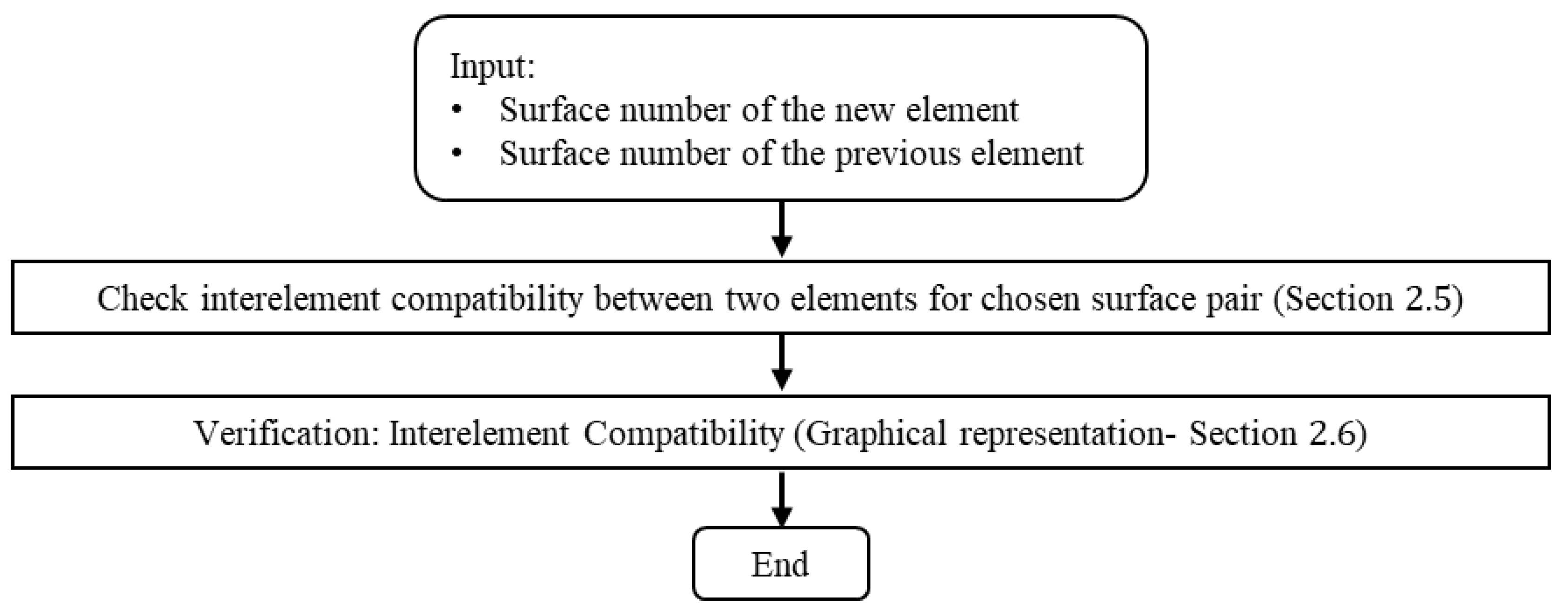
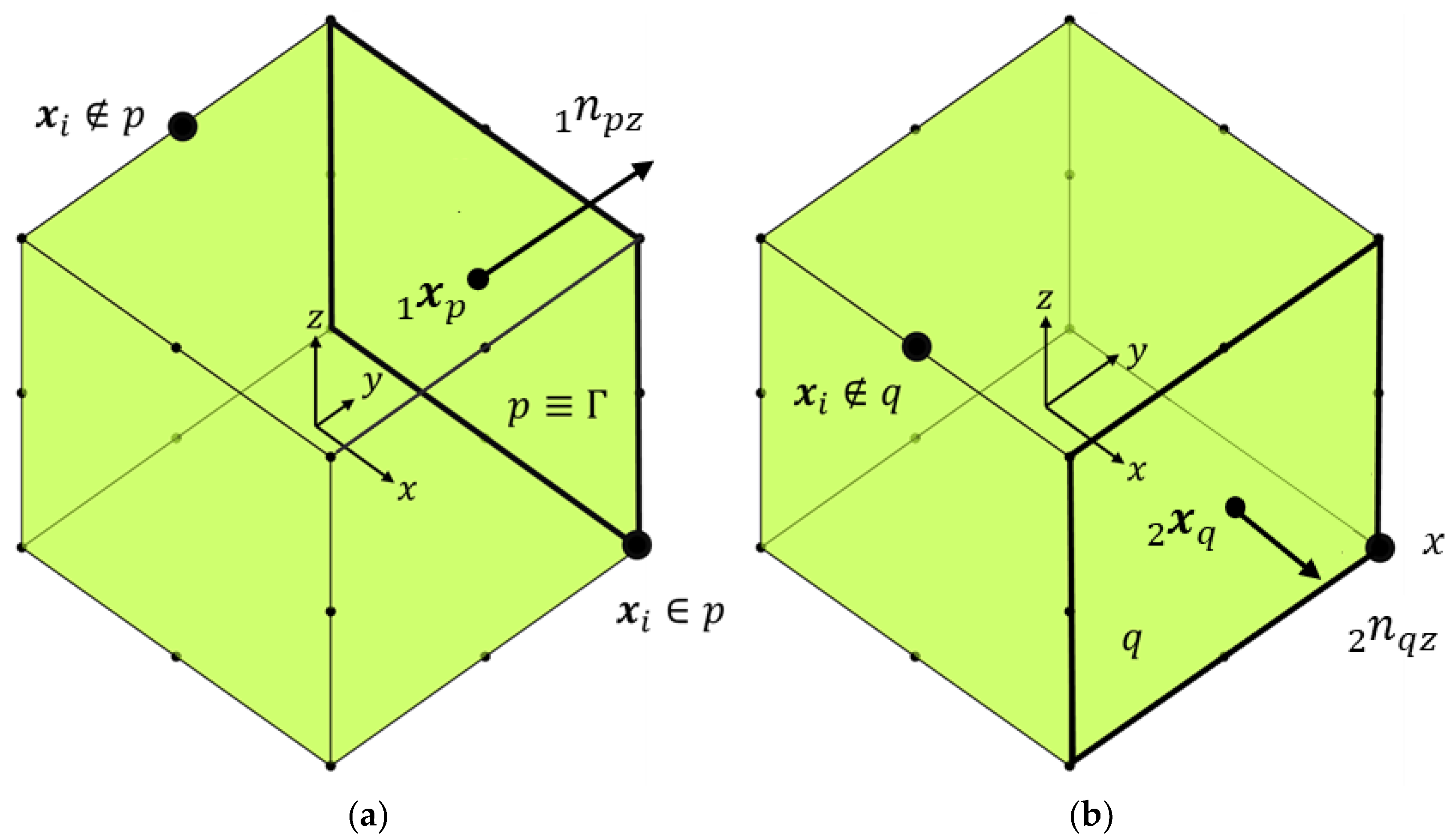
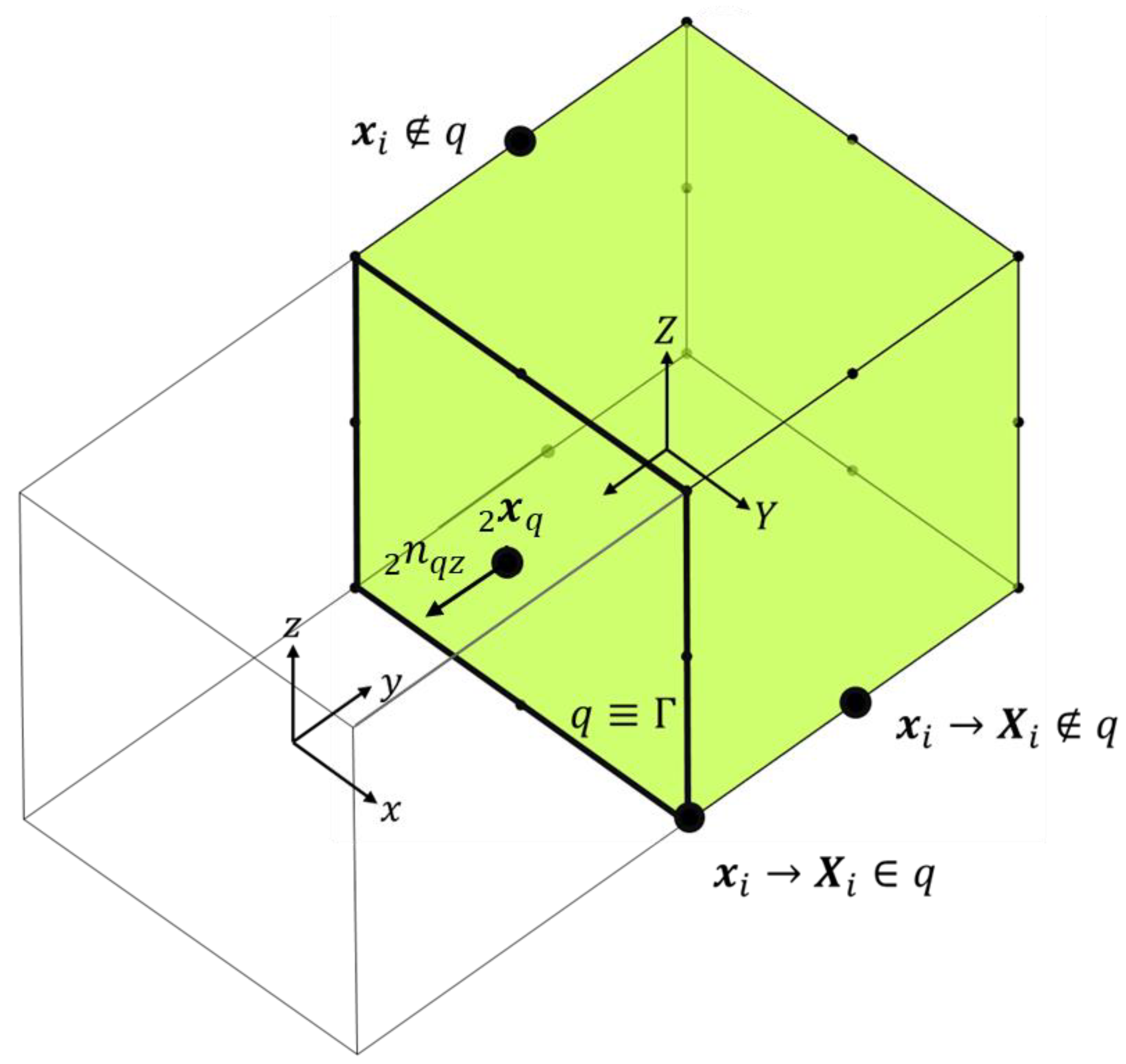
2.5. Interelement Compatibility Check between Two Elements for a Chosen Surface Pair

The nodal compatibility condition requires that the nodal values of a variable evaluated at the common nodes of adjacent elements must be equal. This condition will be satisfied if all the nodes of the interelement surface have the same coordinates and satisfy the interpolation condition. The interelement compatibility condition will be satisfied if the value of a variable is equal for all the points on the interelement surface. If the interelement condition is satisfied, the nodal compatibility condition is satisfied by default. This paper develops a new approach to check the interelement compatibility condition between two elements for a given interelement surface using the symbolic toolbox of Matlab. The approach consists of forming a two-element mesh and ensuring the nodal shapes match at the integration points of the interelement surface.

Assume two elements, $e_1$ and $e_2$, are formulated in the coordinates $\mathit{x}=\left(\begin{array}{ccc}x& y& z\end{array}\right)$, and that the compatibility condition needs to be checked between surface $p$ for element 1 and surface $q$ for element 2. To form an interelement surface $\Gamma$ by $p$ and $q$, element 2 must go through coordinate transformation $(\mathit{x}\to \mathit{X}$) such that the normal surface vectors cancel each other, and the surface centroids have the same coordinates as presented in the equations below

$${}_{p\in 1}{\mathit{n}}_z+{}_{q\in 2}{\mathit{n}}_Z=0$$

(34)

$${}_1{\mathit{x}}_p={}_2{\mathit{X}}_q$$

(35)

A coordinate translation followed by a rotation of the element nodal coordinates is performed to satisfy Equations (34) and (35). Figure 5 presents the elements in the local coordinate $\mathit{x}$, and Figure 6 shows element 2 in the $\mathit{X}$ coordinates after the transformation is conducted. For this purpose, the parametric coordinates of the surfaces of both elements are utilized. A coordinate system,${}_1\mathit{e}$, with $-{}_p{\mathit{n}}_z$ as its third component, indicates that this normal vector points inward to the element as

$${}_1\mathit{e}=\left[\begin{array}{ccc}{}_p{\mathit{n}}_y& {}_p{\mathit{n}}_x& -{}_p{\mathit{n}}_z\end{array}\right]$$

(36)

For element 2, a coordinate system can be constructed as

$${}_2\mathit{e}=\left[\begin{array}{ccc}{}_q{\mathit{n}}_x& {}_q{\mathit{n}}_y& {}_q{\mathit{n}}_z\end{array}\right]$$

(37)

According to Equation (34), element 2 needs to be rotated such that the ${}_q{\mathit{n}}_z$ aligns with $-{}_p{\mathit{n}}_z$. The resulting transformation of the $\mathit{x}$ coordinates is

$$\mathit{X}={}_1\mathit{e}{}_2{\mathit{e}}^T\mathit{x}$$

(38)

Equation (38) facilitates the formation of an interelement boundary between $p$ and $q$. The rotation matrix, ${\mathit{R}}_{\theta }$, about the ${}_q{\mathit{n}}_z$ axis, and the coordinate translation is performed to satisfy Equation (35) as

$$\mathit{X}=\left({}_1\mathit{e}{}_2{\mathit{R}}_{\theta }{\mathit{e}}^T\right)\mathit{x}+\left({}_1{\mathit{x}}_p-{}_2{\mathit{X}}_{Rq}\right)$$

(39)

where ${}_2{\mathit{X}}_{Rq}$ is the centroid of the surface $q$ after coordinate rotation and ${\mathit{R}}_{\theta }$

$${\mathit{R}}_{\theta }=\left[\begin{array}{ccc}cos\theta & -sin\theta & 0\\ sin\theta & cos\theta & 0\\ 0& 0& 1\end{array}\right]$$

(40)

Next, the shape functions are expressed in terms of the global coordinate X following a similar approach as

$$\mathit{X}={\left({}_1\mathit{e}{}_2{\mathit{R}}_{\theta }{\mathit{e}}^T\right)}^T\mathit{x}-\left({}_1{\mathit{x}}_p-{}_2{\mathit{X}}_{Rq}\right)$$

(41)

The variable substitution from x to X is performed using the Symbolic toolbox in Matlab. For an element to undergo such coordinate transformation, x can be mapped (x→X) using isoparametric formulation as,

$$X=\sum _{}^{}{N}_i\left(\mathit{x}\to \mathit{X}\right)x_i$$

(42)

After the coordinate transformation, the compatibility condition can be checked following the procedure presented below. A variable u at x of element 1 can be determined as

$${}_{1}u=\sum _{}^{}{{}_{1}N}_i\left(\mathit{x}\right){}_1{u}_i=\sum _{{\mathit{x}}_j\notin p}^{}{{}_{1}N}_j\left(\mathit{x}\right){}_1{u}_j+\sum _{{\mathit{x}}_k\in p}^{}{{}_{1}N}_k\left(\mathit{x}\right){}_1{u}_k$$

(43)

where ${{}_{1}N}_j$ is shape function $j$ of element 1 and ${\mathit{x}}_j\notin p$ indicates that node $j$ does not fall in the surface $p$. Similarly, a variable u at $\mathit{x}$ of an element 2 can be determined as

$${}_{2}u=\sum _{}^{}{{}_{2}N}_i\left(\mathit{x}\to \mathit{X}\right){}_2{u}_i=\sum _{{\mathit{x}}_j\notin p}^{}{{}_{2}N}_j\left(\mathit{X}\right){}_2{u}_j+\sum _{{\mathit{x}}_k\in p}^{}{{}_{2}N}_k\left(\mathit{X}\right){}_2{u}_k$$

(44)

The interelement compatibility condition holds if the variable ${}_{1}u\left(\mathit{x}\right)={}_{1}u\left(\mathit{X}\right)$, on the interelement surface $\Gamma$. Following Equations (42)–(44) can be written as

$$\begin{gathered} \sum _{{\mathit{x}}_j\notin p}^{}{{}_{1}N}_j\left(\mathit{x}\right){}_1{u}_j+\sum _{{\mathit{x}}_k\in p}^{}{{}_{1}N}_k\left(\mathit{x}\right){}_1{u}_k-\sum _{{\mathit{x}}_l\notin q}^{}{{}_{2}N}_l\left(\mathit{X}\right){}_2{u}_l-\sum _{{\mathit{x}}_m\in q}^{}{{}_{2}N}_m\left(\mathit{X}\right){}_2{u}_m=0 \\ \mathit{x}\in \Gamma \end{gathered}$$

(45)

If the local support condition is satisfied, the first and third components of Equation (45) will be zero as

$$\sum _{{\mathit{x}}_j\notin p}^{}{{}_{1}N}_j\left(\mathit{x}\right){}_1{u}_j=0,\mathit{x}\in \Gamma$$

(46)

$$\sum _{{\mathit{x}}_l\notin q}^{}{{}_{2}N}_l\left(\mathit{X}\right){}_2{u}_l=0,\mathit{x}\in \Gamma$$

(47)

Using Equations (46) and (47) and performing the assembly by setting ${}_2{u}_m={}_1{u}_k={{}_{\Gamma }u}_k$, the compatibility conditions hold if

$$\sum _{{\mathit{x}}_k\in \Gamma }^{}\left({{}_{1}N}_k\left(\mathit{x}\right)-{{}_{2}N}_k\left(\mathit{X}\right)\right){{}_{\Gamma }u}_k=0,\mathit{x}\in \Gamma$$

(48)

For every $\mathit{x}\in \Gamma$, and ${{}_{\Gamma }u}_k$ Equation (46) will be satisfied if

$$\underset{\Gamma }{\overset{}{∯}}\sum _{{\mathit{x}}_k\in \Gamma }^{}{\left({{}_{1}N}_k\left(\mathit{x}\right)-{{}_{2}N}_k\left(\mathit{X}\right)\right)}^{2}d\Gamma =0$$

(49)

Equation (49) can be integrated numerically for each integration point as

$$\sum _{x_g\in \Gamma }^{}\sum _{{\mathit{x}}_k\in \Gamma }^{}{\left({{}_{1}N}_k\left(\mathit{x}\right)-{{}_{2}N}_k\left(\mathit{X}\right)\right)}^2=0$$

(50)

Similarly, Equations (46) and (47) can be checked numerically as

$$\sum _{x_g\in \Gamma }^{}\sum _{{\mathit{x}}_j\notin \Gamma }^{}{\left({{}_{1}N}_j\left(\mathit{x}\right)\right)}^{2}d\Gamma =0$$

(51)

$$\sum _{x_g\in \Gamma }^{}\sum _{{\mathit{x}}_j\notin \Gamma }^{}{\left({{}_{2}N}_j\left(\mathit{X}\right)\right)}^{2}d\Gamma =0$$

(52)

Hence, the compatibility condition is satisfied if Equations (50)–(52) are satisfied for a given element surface pair between two elements.

2.6. Generation of Graphical Representation of Element Properties

Element properties, including (a) shape functions, $N_i$ (b) differentiation of $N_i$ along the x, y, and z-axis, and (c) integration points and weights, are plotted using the Matlab graphics toolbox. These plots facilitate the understanding of the element interpolation function and help to check the interpolation and local support conditions.

The Matlab graphics toolbox is utilized to create a 3D graphical representation of elements’ properties, such as shape function value. For the hexahedron element, the element is subdivided into a 3D grid to perform plotting. For tetrahedrons and arbitrary elements, each surface is plotted. The fidelity of the plot can be increased by discretizing the reference element further by tetrahedron partitioning, and subsequently, each point’s coordinates can be mapped to $S_e$ following Equation (7). Figure 7 presents an example to illustrate the process with a pyramid element. In step 1, the element is subdivided into two tetrahedrons, $S_1$ and $S_2$. In steps 2 and 3, a reference tetrahedron is generated and subdivided into multiple grids to increase the graphics fidelity, and finally, in step 4, each grid point is mapped to the global tetrahedron.

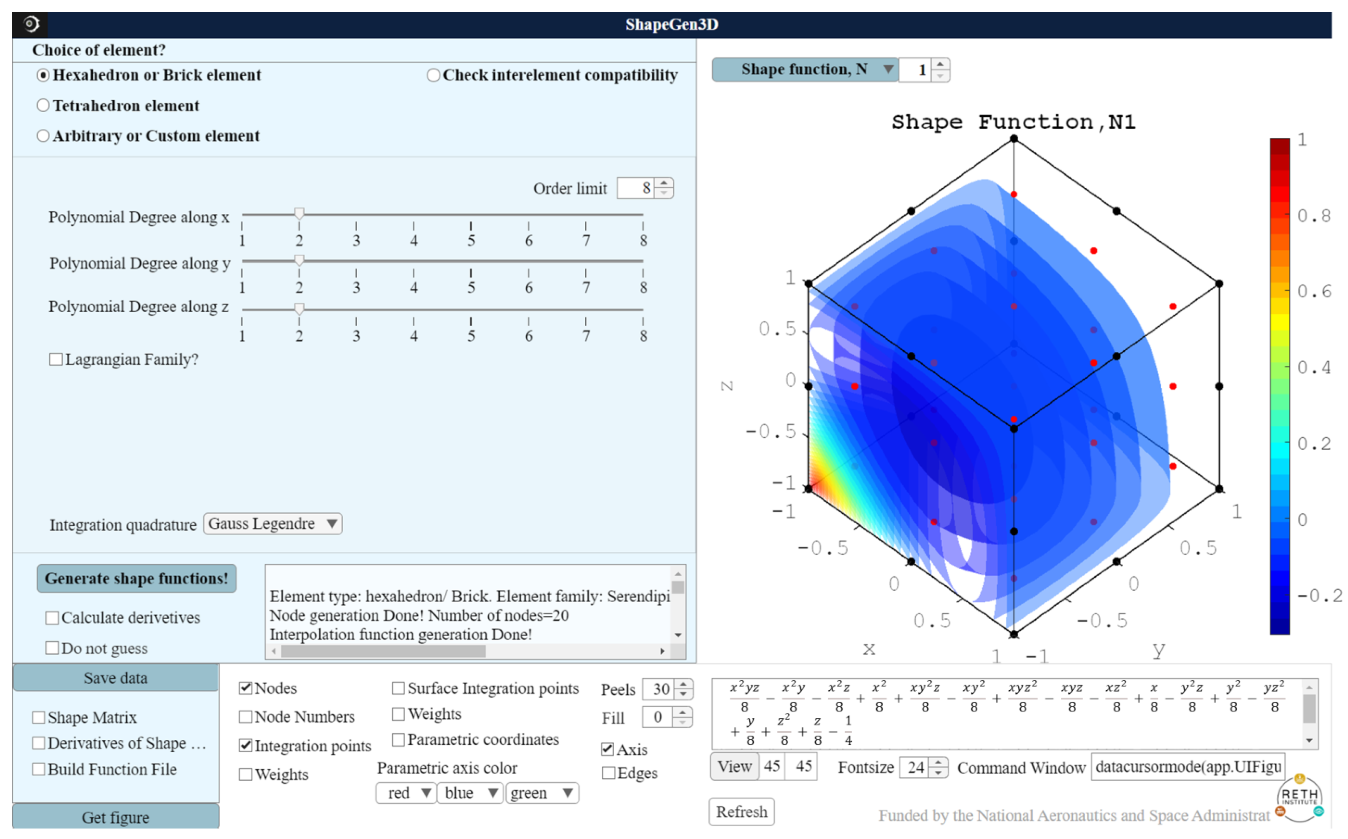
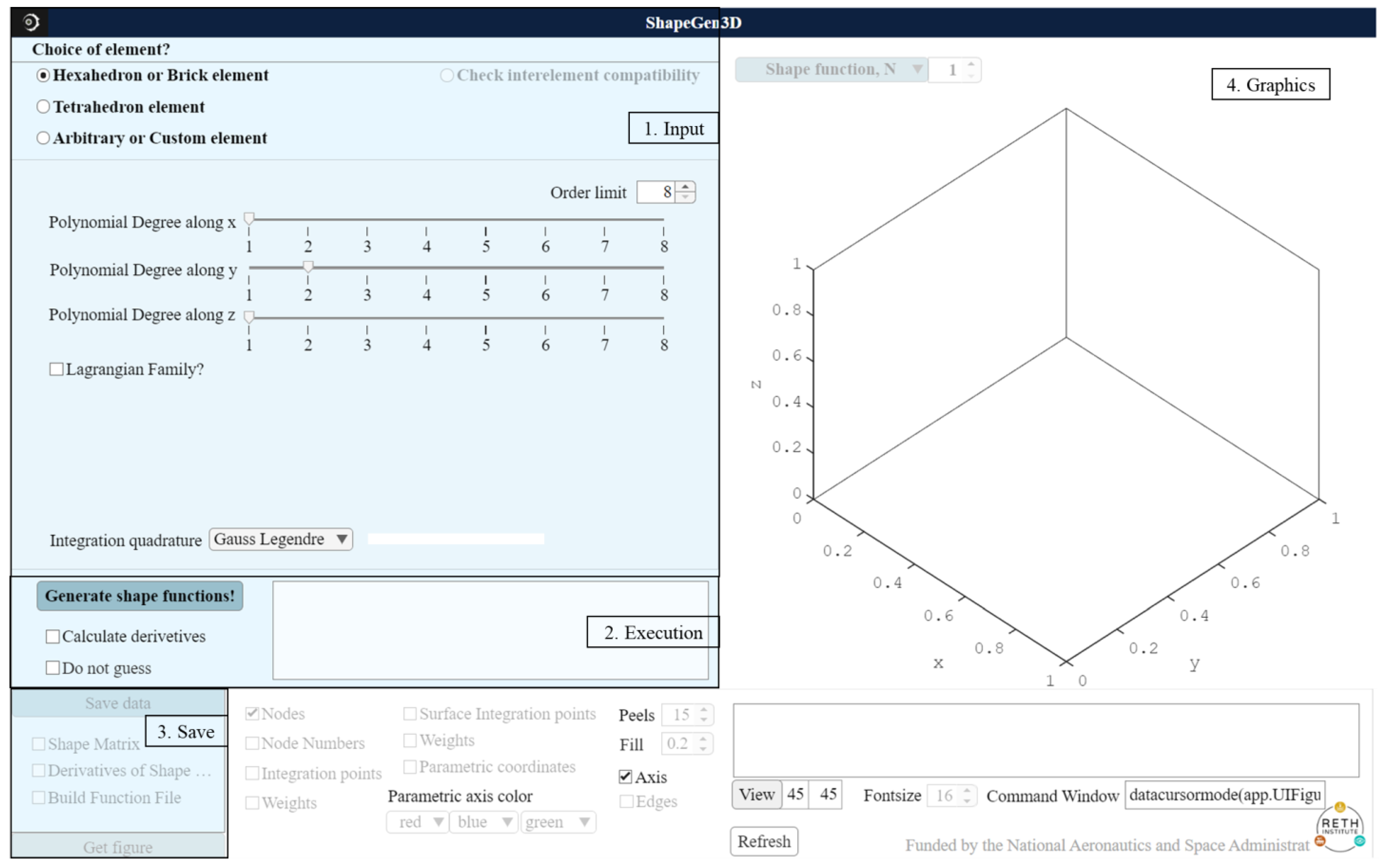
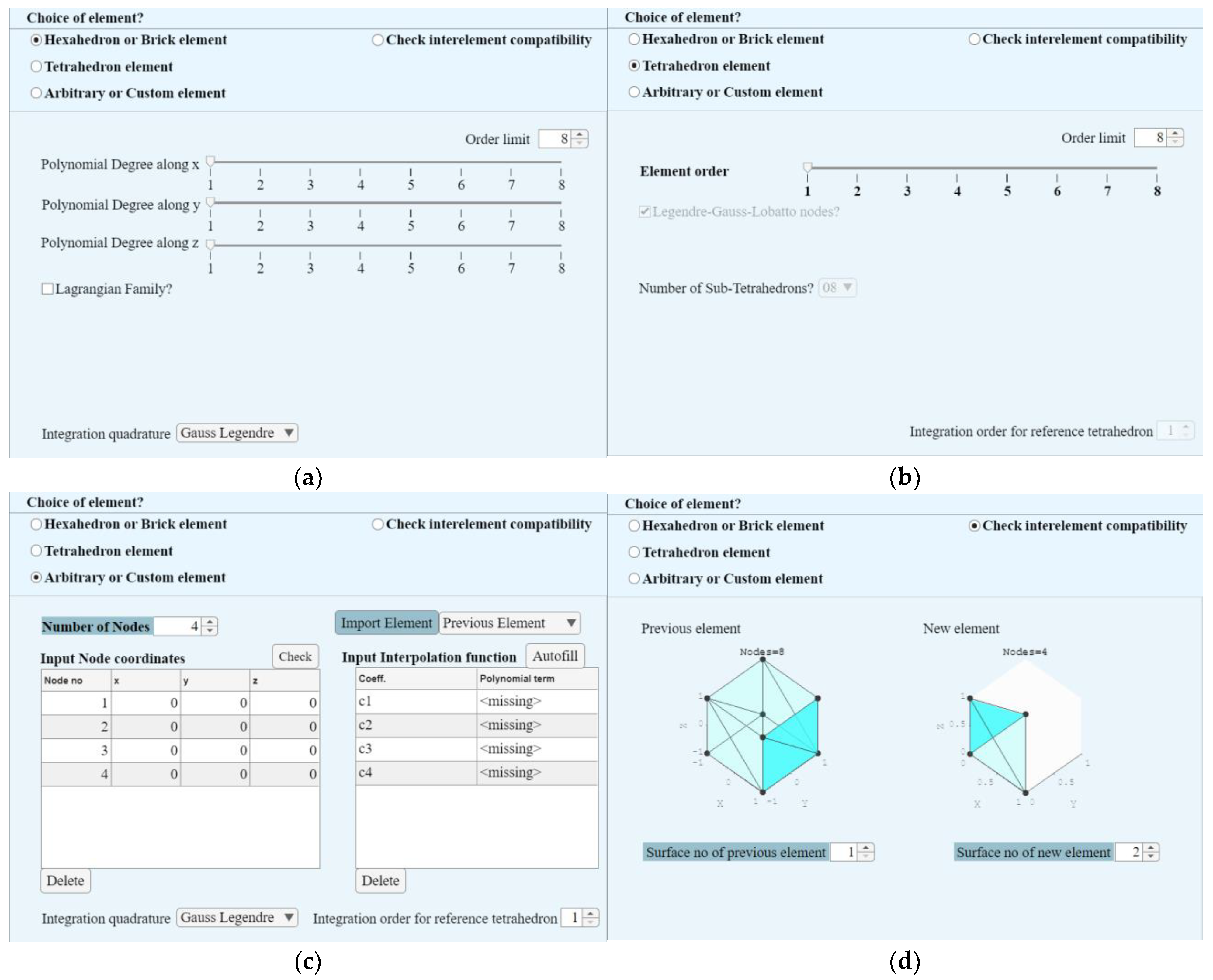
2.7. Implementation of GUI Interface

The procedure is compiled as a GUI software: ShapeGen3D, and organized into four segments, as presented in Figure 8, to enable users to navigate, formulate, and verify the accuracy of the formulation. Segment 1 is the input for the software that lets users choose the element family of interest and the desired interpolation order. Segment 2 includes the execution command to run the software and obtain the element formulation. Segment 3 allows users to store the element properties. Segment 4 represents the results and post-processing blocks that will enable users to observe and manipulate plots that can be used to verify the accuracy of the generated formulation visually. Detailed descriptions for each of these segments are provided below.

A short description and a screenshot of the sub-options in Segment 1 are presented in

Table 3. Segment 1 sub-options and description.

Seg 1: Input Options	Sub-Options	Description
Hexahedron or Brick element	Polynomial degree along $x$	$m_x$ of Equation (17)
	Polynomial degree along $y$	$m_y$ of Equation (18)
	Polynomial degree along $z$	$m_z$ of Equation (19)
	Lagrangian Family	Checking this option will formulate a Lagrangian element. Otherwise, a Serendipity element will be formulated
	Integration quadrature	This option offers two integration quadratures; (1) Gauss–Legendre (2) Gauss–Lobatto
Tetrahedron element	Element order	$m$ in Equation (27)
	Number of Sub-Tetrahedral	The number of sub-tetrahedrons used for integration quadrature following the finite cell method. It is active when an element order greater than 4 is used.
	Integration order for reference tetrahedron	The integration order for each sub-tetrahedron. It is active when an element order greater than 4 is used.
Arbitrary or Custom element	Input node coordinates	A table where the user can input the nodal distribution of the desired element and cartesian coordinates (x, y, z) for each node.
	Input interpolation function	A table where the user can input $F_i\left(x,y,z\right)$ from Equation (3), where $i=\left[1d\right]$ and $d$ is the number of nodes.
	Integration quadrature	If the software detects an arbitrary element from the isoparametric hexahedron family, it will determine the selected integration quadrature from one of the selected options: (1) Gauss–Legendre and (2) Gauss–Lobatto.
	Integration order for reference tetrahedron	If the element is not from an isoparametric hexahedron family, the integration quadrature is determined following the procedure presented in Section 2.2 with the integration order selected in this option
Check interelement compatibility		Used to illustrate two consecutively generated elements

and Figure 9, respectively. The element order and integration quadrature type must be defined for developing hexahedron and tetrahedron elements. On the other hand, in the case of arbitrary or custom elements, the nodal distribution must be inputted by users, and the software will determine the integration quadrature.

Segment 2 represents the “Execution” block. It includes the “Generate shape function” button, which executes the code with the input given in Segment 1 and generates shape functions, integration quadrature, and graphical representation of the element properties. The code can automatically detect isoparametric hexahedrons and tetrahedron elements. There are several checkboxes, such as the “Do not guess” command. If this box is checked, the software avoids detecting the element type and assumes it is an arbitrary element. This segment also includes a display window that shows messages and the progress of the execution of the code. If the “Check interelement compatibility” box is selected in Segment 1, this option will be activated in Segment 2. The software will compute the nodes with the same coordinates between two consecutive elements and subtract the corresponding shape functions. If the difference is 0 at an interelement boundary, that boundary satisfies the compatibility condition between two elements, i.e., there are no discontinuities at the boundary.

Segment 3 is a block that outputs results in the Matlab workspace to allow users to implement the elements in other programming languages or through user elements in commercial finite element software, such as ABAQUS and ANSYS. Users can also output shape functions and derivatives of the shape functions evaluated at the integration points by ticking the “Shape matrix” and “Derivatives of Shape matrix” options. A description of the workspace files is presented in

Table 4. Output files to Matlab workspace.

Workspace Filename	Description	Data Structure
Interpolation_Functions	Stores interpolation in symbolic format	$\left[\begin{array}{cccc}{F}_1& F_2& .& F_d\end{array}\right]$ $F_i$: Function I of Equation 1 in symbolic format
Node_Coordinates	Stores node coordinates	$\left[\begin{array}{ccc}{n}_{x_1}& n_{y_1}& n_{z_1}\\ n_{x_2}& n_{y_2}& n_{z_2}\\ .& .& .\\ n_{x_d}& n_{y_d}& n_{z_d}\end{array}\right]$ $n_j(n_{x_i},n_{y_i},n_{z_i})$ where $n_{x_i}$: $x$ coordinate of node $i$ .
Shape_Functions	Stores shape functions in symbolic format for the corresponding nodes	$\left[\begin{array}{c}{N}_1\\ N_2\\ .\\ N_d\end{array}\right]$ $N_i$: Shape function $i$ in symbolic format.
Surface_Nodes_and_vectors	Stores nodes on surface and surface normal vector pointing outward of the domain for all surfaces	$\left[\begin{array}{cccc}a& n_{x_a}& n_{y_a}& n_{z_a}\\ b& n_{x_b}& n_{y_b}& n_{z_b}\\ .& .& .& .\\ d& n_{x_d}& n_{y_d}& n_{z_d}\end{array}\right]$ $a,b,d$ are node numbers and integers. $n_j(n_{x_j},n_{y_j},n_{z_j})$ is the normal vector pointing outward of the domain on the surface containing node $j$.
Integration_Points_Coordinates_Weights	Stores integration points and weights inside the element	$\left[\begin{array}{cccc}{g}_{x_1}& g_{y_1}& g_{z_1}& w_1\\ g_{x_2}& g_{y_2}& g_{z_2}& w_2\\ .& .& .& .\\ g_{x_d}& g_{y_d}& g_{z_d}& w_d\end{array}\right]$ $g_j(g_{x_j},g_{y_j},g_{z_j})$ where $g_{x_j}:$ $x$ coordinate of integration point $j$. $w_j$: weight of integration point $j$.
Integration_Points_Coordinates_Weights_Vectors on_Surface	Stores integration points and weights on surfaces and surface normal vector pointing outward of the domain for all surfaces	$\left[\begin{array}{cccc}{g}_{x_1}& g_{y_1}& g_{z_1}& w_1\\ g_{x_2}& g_{y_2}& g_{z_2}& w_2\\ .& .& .& .\\ g_{x_d}& g_{y_d}& g_{z_d}& w_d\end{array}\right]\left[\begin{array}{ccc}{n}_{x_1}& n_{y_1}& n_{z_1}\\ n_{x_2}& n_{y_2}& n_{z_2}\\ .& .& .\\ n_{x_d}& n_{y_d}& n_{z_d}\end{array}\right]$ $g_j(g_{x_j},g_{y_j},g_{z_j})$ where $g_{x_j}$: $x$ coordinate of integration point $j$. $w_j$: weight of integration point. $j.$ $n_j(n_{x_j},n_{y_j},n_{z_j})$ is the normal unit vector pointing outward of the domain on the surface at integration point $j$.
Parametric_Coordinates	Stores parametric coordinates for each surface of the element	${\left[\begin{array}{cc}{n}_{x_1}& n_{y_1}\\ n_{x_2}& n_{y_2}\\ n_{x_3}& n_{y_3}\end{array}\right]}_S$ $n_{x_j}$ and $n_{y_j}$ are the parametric $x$ and y coordinates, respectively. $S$ represents the surface number.
Shape_Matrix	Stores the value of each shape function evaluated at each integration point	$\left[\begin{array}{cccc}{\left.N_1\right|}_{g_1}& {\left.N_2\right|}_{g_1}& .& {\left.N_n\right|}_{g_d}\\ {\left.N_1\right|}_{g_2}& {\left.N_2\right|}_{g_2}& .& {\left.N_n\right|}_{g_d}\\ .& .& .& .\\ {\left.N_1\right|}_{g_n}& {\left.N_2\right|}_{g_d}& .& {\left.N_n\right|}_{g_d}\end{array}\right]$ ${\left.N_i\right|}_{g_j}$: shape function $i$ evaluated at integration point $j$.
dx_Shape_Matrix	Stores the value of the first derivative of each shape function evaluated at each integration point	$\left[\begin{array}{cccc}{\left.\frac{\partial N_1}{\partial x}\right|}_{g_1}& {\left.\frac{\partial N_2}{\partial x}\right|}_{g_1}& .& {\left.\frac{\partial N_n}{\partial x}\right|}_{g_1}\\ {\left.\frac{\partial N_1}{\partial x}\right|}_{g_2}& {\left.\frac{\partial N_2}{\partial x}\right|}_{g_2}& .& {\left.\frac{\partial N_n}{\partial x}\right|}_{g_2}\\ .& .& .& .\\ {\left.\frac{\partial N_1}{\partial x}\right|}_{g_n}& {\left.\frac{\partial N_2}{\partial x}\right|}_{g_n}& .& {\left.\frac{\partial N_n}{\partial x}\right|}_{g_n}\end{array}\right]$ ${\left.\frac{\partial N_i}{\partial x}\right|}_{g_j}$: shape function derivative $i$ evaluated at integration point $j$.

. These files are readily available for FEM calculations.

Finally, segment 4 represents a results and post-processing block that shows the results obtained by the software and allows users to manipulate graphics. There are many components, such as the “Shape function, N” spinner block, which is a control block where the user can select to plot the number of shape function properties, such as their value and derivatives. This segment also allows users to plot other element properties, such as node number, integration points, and weights, as shown in the bottom left part of the software. It also includes a display window that shows the shape function property in equation format and other user-controlled options to manipulate the graphics options, such as the view angle, axis, image resolution (Peels), and transparency (Fill). Increasing the “Peels” will increase the overall image resolution. If “Fill” is chosen as 0, the software will not show any 0 value and will represent it as a blank space.

3. Numerical Examples

This section shows the properties of three different 3D elements that were obtained following the procedure developed in this paper. The results were generated through the GUI software: ShapeGen3D. First, the element properties, i.e., nodal coordinates, shape functions, and integration quadrature, of the popular 20-node brick element were obtained and compared against the literature to verify the accuracy of the formulation. Second, a 21-node hexahedron transition element similar to a 20-node quadratic hexahedron element but with one node on the $xy$ face at $z=1$ was formulated. The interpolation, local support condition, and compatibility with the 20-node brick element were checked. Third, a custom element was formulated to replicate the Germain–Lagrange plate [41] bending, showing how the methodology implemented in the software can help solve challenging problems efficiently. The fourth example shows the development of a 43-node transition element from a fourth to second-order Lagrangian element. Finally, two high-order spectral elements were formulated to provide a complete overview. The steps followed in ShapeGen3D to generate the elements’ shape functions and other finite element properties for each of the examples are presented in

Table A9. Element formulation steps.

Objective	Procedure
20-node brick formulation	Segment 1 options	Hexahedron or Brick element	Click
		Polynomial degree along $x$	2
		Polynomial degree along $y$	2
		Polynomial degree along $z$	2
		Lagrangian Family	Un-check
		Integration quadrature	Gauss–Legendre
	Segment 2 options	Do not guess	Unchecked
		Generate shape function!	Click
21-node brick formulation	Segment 1 options	Arbitrary or Custom element	Click
		Import Element	Previous Element
		Number of nodes	21
		Input Node coordinates in the 21st row	0 0 1
		Input Interpolation function in the 21st row	$x^2{y}^2(z+1)$
		Integration quadrature	Gauss–Legendre
	Segment 2 options	Do not guess	Unchecked
		Generate shape function!	Click
20 and 21-node brick compatibility test	Segment 1 options	Compare shape function	Click
		Check interelement compatibility	Click
36-node brick element	Segment 1 options	Hexahedron or Brick element	Click
		Polynomial degree along $x$	4
		Polynomial degree along $y$	4
		Polynomial degree along $z$	2
		Lagrangian Family	Un-check
		Integration quadrature	Gauss–Legendre
	Segment 2 options	Do not guess	Unchecked
		Generate shape function!	Click
43-node brick element for Germain–Lagrange plate bending	Segment 1 options	Arbitrary or Custom element	Click
		Import Element	Previous Element
		Number of nodes	43
		Input Node coordinates	0 0 1
			0 0 −1
			0 1 0
			0 −1 0
			1 0 0
			−1 0 0
			0 0 0
		Input monomial basis functions	$x^2{y}^2{z}^2$
			$x^2{y}^{2}z$
			$x^{2}y{z}^2$
			$x{y}^2{z}^2$
			$x^2{y}^2$
			$z^2{y}^2$
			$x^2{z}^2$
		Integration quadrature	Gauss–Legendre
	Segment 2 options	Do not guess	Unchecked
		Generate shape function!	Click
75-node brick element	Segment 1 options	Hexahedron or Brick element	Click
		Polynomial degree along $x$	4
		Polynomial degree along $y$	4
		Polynomial degree along $z$	2
		Lagrangian Family	Check
		Integration quadrature	Gauss–Lobatto
	Segment 2 options	Do not guess	Unchecked
		Generate shape function!	Click
43-node transition element from fourth to second order Lagrangian element	Segment 1 options	Arbitrary or Custom element	Click
		Import Element	Previous Element
		Number of nodes	43
		Remove Node coordinates	0 0 1
			0 0 −1
			0 1 0
			0 −1 0
			1 0 0
			−1 0 0
			0 0 0
		Remove monomial basis functions	Factors with $$\begin{gathered} m_x<3 \\ {m}_y<3 \\ {m}_z<3 \end{gathered}$$
		Modify monomial basis functions	$x^3\left(z+1\right)$
			$y^3\left(z+1\right)$
			$x^4\left(z+1\right)$
			$x^{3}y\left(z+1\right)$
			$y^3\left(z+1\right)$
			$y^4\left(z+1\right)$
			$x^{4}y\left(z+1\right)$
			$x^3{y}^2\left(z+1\right)$
		Integration quadrature	Gauss–Lobatto
	Segment 2 options	Do not guess	Unchecked
		Generate shape function!	Click
Spectral hexahedron formulation	Segment 1 options	Hexahedron or Brick element	Click
		Polynomial degree along $x$	5
		Polynomial degree along $y$	5
		Polynomial degree along $z$	2
		Lagrangian Family	Check
		Integration quadrature	Gauss–Lobatto
	Segment 2 options	Do not guess	Unchecked
		Generate shape function!	Click
Spectral tetrahedron formulation	Segment 1 options	Tetrahedron element	Click
		Element order	5
		No of Sub-Tetrahedrons	8
		Integration order for reference tetrahedron	1
	Segment 2 options	Do not guess	Unchecked
		Generate shape function!	Click

.

3.1. 20-Node Brick Element

A 20-node brick element follows serendipity element formulation with $m_x$ = 2, $m_y$ = 2, and $m_z$ = 2. The software determines the nodal coordinates, shape functions (Stage 1), and integration quadrature (Stage 2). The obtained results were saved as the files explained in Table 4 and are shown in the Appendix A, see

Table A1. Node_Coordinates for 20 node brick element.

Node Number	X	y	Z
1	−1	−1	−1
2	1	−1	−1
3	1	1	−1
4	−1	1	−1
5	−1	−1	1
6	1	−1	1
7	1	1	1
8	−1	1	1
9	0	−1	−1
10	1	0	−1
11	0	1	−1
12	−1	0	−1
13	0	−1	1
14	1	0	1
15	0	1	1
16	−1	0	1
17	−1	−1	0
18	1	−1	0
19	1	1	0
20	−1	1	0

,

Table A2. Shape_Functions for 20-node brick element.

Node	${\mathit{N}}_{\mathit{i}}(\mathit{x},\mathit{y},\mathit{z})$
1	$\frac{x^{2}yz}{8}-\frac{x^{2}y}{8}-\frac{x^{2}z}{8}+\frac{x^2}{8}+\frac{x{y}^{2}z}{8}-\frac{x{y}^2}{8}+\frac{xy{z}^2}{8}-\frac{xyz}{8}-\frac{x{z}^2}{8}+\frac{x}{8}-\frac{y^{2}z}{8}+\frac{y^2}{8}-\frac{y{z}^2}{8}+\frac{y}{8}+\frac{z^2}{8}+\frac{z}{8}-\frac{1}{4}$
2	$\frac{x^{2}yz}{8}-\frac{x^{2}y}{8}-\frac{x^{2}z}{8}+\frac{x^2}{8}-\frac{x{y}^{2}z}{8}+\frac{x{y}^2}{8}-\frac{xy{z}^2}{8}+\frac{xyz}{8}+\frac{x{z}^2}{8}-\frac{x}{8}-\frac{y^{2}z}{8}+\frac{y^2}{8}-\frac{y{z}^2}{8}+\frac{y}{8}+\frac{z^2}{8}+\frac{z}{8}-\frac{1}{4}$
3	$-\frac{x^{2}yz}{8}+\frac{x^{2}y}{8}-\frac{x^{2}z}{8}+\frac{x^2}{8}-\frac{x{y}^{2}z}{8}+\frac{x{y}^2}{8}+\frac{xy{z}^2}{8}-\frac{xyz}{8}+\frac{x{z}^2}{8}-\frac{x}{8}-\frac{y^{2}z}{8}+\frac{y^2}{8}+\frac{y{z}^2}{8}-\frac{y}{8}+\frac{z^2}{8}+\frac{z}{8}-\frac{1}{4}$
4	$-\frac{x^{2}yz}{8}+\frac{x^{2}y}{8}-\frac{x^{2}z}{8}+\frac{x^2}{8}+\frac{x{y}^{2}z}{8}-\frac{x{y}^2}{8}-\frac{xy{z}^2}{8}+\frac{xyz}{8}-\frac{x{z}^2}{8}+\frac{x}{8}-\frac{y^{2}z}{8}+\frac{y^2}{8}+\frac{y{z}^2}{8}-\frac{y}{8}+\frac{z^2}{8}+\frac{z}{8}-\frac{1}{4}$
5	$-\frac{x^{2}yz}{8}+\frac{x^{2}y}{8}-\frac{x^{2}z}{8}+\frac{x^2}{8}-\frac{x{y}^{2}z}{8}+\frac{x{y}^2}{8}+\frac{xy{z}^2}{8}-\frac{xyz}{8}+\frac{x{z}^2}{8}-\frac{x}{8}-\frac{y^{2}z}{8}+\frac{y^2}{8}+\frac{y{z}^2}{8}-\frac{y}{8}+\frac{z^2}{8}+\frac{z}{8}-\frac{1}{4}$
6	$-\frac{x^{2}yz}{8}+\frac{x^{2}y}{8}-\frac{x^{2}z}{8}+\frac{x^2}{8}+\frac{x{y}^{2}z}{8}-\frac{x{y}^2}{8}-\frac{xy{z}^2}{8}+\frac{xyz}{8}-\frac{x{z}^2}{8}+\frac{x}{8}-\frac{y^{2}z}{8}+\frac{y^2}{8}+\frac{y{z}^2}{8}-\frac{y}{8}+\frac{z^2}{8}+\frac{z}{8}-\frac{1}{4}$
7	$-\frac{x^{2}yz}{8}-\frac{x^{2}y}{8}+\frac{x^{2}z}{8}+\frac{x^2}{8}-\frac{x{y}^{2}z}{8}-\frac{x{y}^2}{8}+\frac{xy{z}^2}{8}+\frac{xyz}{8}-\frac{x{z}^2}{8}+\frac{x}{8}+\frac{y^{2}z}{8}+\frac{y^2}{8}-\frac{y{z}^2}{8}+\frac{y}{8}+\frac{z^2}{8}-\frac{z}{8}-\frac{1}{4}$
8	$-\frac{x^{2}yz}{8}-\frac{x^{2}y}{8}+\frac{x^{2}z}{8}+\frac{x^2}{8}+\frac{x{y}^{2}z}{8}+\frac{x{y}^2}{8}-\frac{xy{z}^2}{8}-\frac{xyz}{8}+\frac{x{z}^2}{8}-\frac{x}{8}+\frac{y^{2}z}{8}+\frac{y^2}{8}-\frac{y{z}^2}{8}+\frac{y}{8}+\frac{z^2}{8}-\frac{z}{8}-\frac{1}{4}$
9	$\frac{yz}{4}-\frac{z}{4}-\frac{y}{4}+\frac{x^{2}y}{4}+\frac{x^{2}z}{4}-\frac{x^2}{4}-\frac{x^{2}yz}{4}+\frac{1}{4}$
10	$\frac{x}{4}-\frac{z}{4}-\frac{xz}{4}-\frac{x{y}^2}{4}+\frac{y^{2}z}{4}-\frac{y^2}{4}+\frac{x{y}^{2}z}{4}+\frac{1}{4}$
11	$\frac{y}{4}-\frac{z}{4}-\frac{yz}{4}-\frac{x^{2}y}{4}+\frac{x^{2}z}{4}-\frac{x^2}{4}+\frac{x^{2}yz}{4}+\frac{1}{4}$
12	$\frac{xz}{4}-\frac{z}{4}-\frac{x}{4}+\frac{x{y}^2}{4}+\frac{y^{2}z}{4}-\frac{y^2}{4}-\frac{x{y}^{2}z}{4}+\frac{1}{4}$
13	$\frac{z}{4}-\frac{y}{4}-\frac{y*z}{4}+\frac{x^{2}y}{4}-\frac{x^{2}z}{4}-\frac{x^2}{4}+\frac{x^{2}yz}{4}+\frac{1}{4}$
14	$\frac{x}{4}+\frac{z}{4}+\frac{xz}{4}-\frac{x{y}^2}{4}-\frac{y^{2}z}{4}-\frac{y^2}{4}-\frac{x{y}^{2}z}{4}+\frac{1}{4}$
15	$\frac{y}{4}+\frac{z}{4}+\frac{yz}{4}-\frac{x^{2}y}{4}-\frac{x^{2}z}{4}-\frac{x^2}{4}-\frac{x^{2}yz}{4}+\frac{1}{4}$
16	$\frac{z}{4}-\frac{x}{4}-\frac{xz}{4}+\frac{x{y}^2}{4}-\frac{y^{2}z}{4}-\frac{y^2}{4}+\frac{x{y}^{2}z}{4}+\frac{1}{4}$
17	$\frac{xy}{4}-\frac{y}{4}-\frac{x}{4}+\frac{x{z}^2}{4}+\frac{y{z}^2}{4}-\frac{z^2}{4}-\frac{xy{z}^2}{4}+\frac{1}{4}$
18	$\frac{x}{4}-\frac{y}{4}-\frac{xy}{4}-\frac{x{z}^2}{4}+\frac{y{z}^2}{4}-\frac{z^2}{4}+\frac{xy{z}^2}{4}+\frac{1}{4}$
19	$\frac{x}{4}+\frac{y}{4}+\frac{xy}{4}-\frac{x{z}^2}{4}-\frac{y{z}^2}{4}-\frac{z^2}{4}-\frac{xy{z}^2}{4}+\frac{1}{4}$
20	$\frac{y}{4}-\frac{x}{4}-\frac{xy}{4}+\frac{x{z}^2}{4}-\frac{y{z}^2}{4}-\frac{z^2}{4}+\frac{xy{z}^2}{4}+\frac{1}{4}$

,

Table A3. Integration_Points_Coordinates and Integration_Points_Weights for 20 node brick element.

Integration Point No	x	y	z	Weight
1	−0.7746	−0.7746	−0.7746	0.171468
2	−0.7746	−0.7746	0	0.274348
3	−0.7746	−0.7746	0.774597	0.171468
4	−0.7746	0	−0.7746	0.274348
5	−0.7746	0	0	0.438957
6	−0.7746	0	0.774597	0.274348
7	−0.7746	0.774597	−0.7746	0.171468
8	−0.7746	0.774597	0	0.274348
9	−0.7746	0.774597	0.774597	0.171468
10	0	−0.7746	−0.7746	0.274348
11	0	−0.7746	0	0.438957
12	0	−0.7746	0.774597	0.274348
13	0	0	−0.7746	0.438957
14	0	0	0	0.702332
15	0	0	0.774597	0.438957
16	0	0.774597	−0.7746	0.274348
17	0	0.774597	0	0.438957
18	0	0.774597	0.774597	0.274348
19	0.774597	−0.7746	−0.7746	0.171468
20	0.774597	−0.7746	0	0.274348
21	0.774597	−0.7746	0.774597	0.171468
22	0.774597	0	−0.7746	0.274348
23	0.774597	0	0	0.438957
24	0.774597	0	0.774597	0.274348
25	0.774597	0.774597	−0.7746	0.171468
26	0.774597	0.774597	0	0.274348
27	0.774597	0.774597	0.774597	0.171468

,

Table A4. Integration_Points_Coordinates_Weights_Vectors_on_Surface for 20 node brick element.

Integration Point No	x	y	z	Weight	${\mathit{n}}_{\mathit{x}}$	${\mathit{n}}_{\mathit{y}}$	${\mathit{n}}_{\mathit{z}}$
1	1	−0.7746	−0.7746	0.30864	1	0	0
2	1	−0.7746	0	0.49382	1	0	0
3	1	−0.7746	0.77459	0.30864	1	0	0
4	1	0	−0.7746	0.49382	1	0	0
5	1	0	0	0.79012	1	0	0
6	1	0	0.77459	0.49382	1	0	0
7	1	0.77459	−0.7746	0.30864	1	0	0
8	1	0.77459	0	0.49382	1	0	0
9	1	0.77459	0.77459	0.30864	1	0	0
10	−1	−0.7746	−0.7746	0.30864	−1	0	0
11	−1	−0.7746	0	0.49382	−1	0	0
12	−1	−0.7746	0.77459	0.30864	−1	0	0
13	−1	0	−0.7746	0.49382	−1	0	0
14	−1	0	0	0.79012	−1	0	0
15	−1	0	0.77459	0.49382	−1	0	0
16	−1	0.77459	−0.7746	0.30864	−1	0	0
17	−1	0.77459	0	0.49382	−1	0	0
18	−1	0.77459	0.77459	0.30864	−1	0	0
19	−0.7746	1	−0.7746	0.30864	0	1	0
20	−0.7746	1	0	0.49382	0	1	0
21	−0.7746	1	0.77459	0.30864	0	1	0
22	0	1	−0.7746	0.49382	0	1	0
23	0	1	0	0.79012	0	1	0
24	0	1	0.77459	0.49382	0	1	0
25	0.77459	1	−0.7746	0.30864	0	1	0
26	0.77459	1	0	0.49382	0	1	0
27	0.77459	1	0.77459	0.30864	0	1	0
28	−0.7746	−1	−0.7746	0.30864	0	−1	0
29	−0.7746	−1	0	0.49382	0	−1	0
30	−0.7746	−1	0.77459	0.30864	0	−1	0
31	0	−1	−0.7746	0.49382	0	−1	0
32	0	−1	0	0.79012	0	−1	0
33	0	−1	0.77459	0.49382	0	−1	0
34	0.77459	−1	−0.7746	0.30864	0	−1	0
35	0.77459	−1	0	0.49382	0	−1	0
36	0.77459	−1	0.77459	0.30864	0	−1	0
37	−0.7746	−0.7746	1	0.30864	0	0	1
38	−0.7746	0	1	0.49382	0	0	1
39	−0.7746	0.77459	1	0.30864	0	0	1
40	0	−0.7746	1	0.49382	0	0	1
41	0	0	1	0.79012	0	0	1
42	0	0.77459	1	0.49382	0	0	1
43	0.77459	−0.7746	1	0.30864	0	0	1
44	0.77459	0	1	0.49382	0	0	1
45	0.77459	0.77459	1	0.30864	0	0	1
46	−0.7746	−0.7746	−1	0.30864	0	0	−1
47	−0.7746	0	−1	0.49382	0	0	−1
48	−0.7746	0.77459	−1	0.30864	0	0	−1
49	0	−0.7746	−1	0.49382	0	0	−1
50	0	0	−1	0.79012	0	0	−1
51	0	0.77459	−1	0.49382	0	0	−1
52	0.77459	−0.7746	−1	0.30864	0	0	−1
53	0.77459	0	−1	0.49382	0	0	−1
54	0.77459	0.77459	−1	0.30864	0	0	−1

and

Table A5. Surface_Nodes_and_vectors for 20-node brick element.

Node Number	${\mathit{n}}_{\mathit{x}}$	${\mathit{n}}_{\mathit{y}}$	${\mathit{n}}_{\mathit{z}}$
2	1	0	0
3	1	0	0
6	1	0	0
7	1	0	0
10	1	0	0
14	1	0	0
18	1	0	0
19	1	0	0
1	−1	0	0
4	−1	0	0
5	−1	0	0
8	−1	0	0
12	−1	0	0
16	−1	0	0
17	−1	0	0
20	−1	0	0
3	0	1	0
4	0	1	0
7	0	1	0
8	0	1	0
11	0	1	0
15	0	1	0
19	0	1	0
20	0	1	0
1	0	−1	0
2	0	−1	0
5	0	−1	0
6	0	−1	0
9	0	−1	0
13	0	−1	0
17	0	−1	0
18	0	−1	0
5	0	0	1
6	0	0	1
7	0	0	1
8	0	0	1
13	0	0	1
14	0	0	1
15	0	0	1
16	0	0	1
1	0	0	−1
2	0	0	−1
3	0	0	−1
4	0	0	−1
9	0	0	−1
10	0	0	−1
11	0	0	−1
12	0	0	−1

, which includes: (1) nodal coordinates; (2) corresponding shape functions; (3) integration points and weights; (4) integration points on the surface and weights; and (5) nodes on the surface and surface normal vector pointing outward of the domain for all surfaces, respectively. The nodal coordinates, shape functions, and integration quadrature match the formulation found in the literature [37], thus verifying the accuracy of the software results. Figure 10 represents the input to the ShapeGen3D and the obtained results with nodes as black dots and integration points for volume integration as red dots.

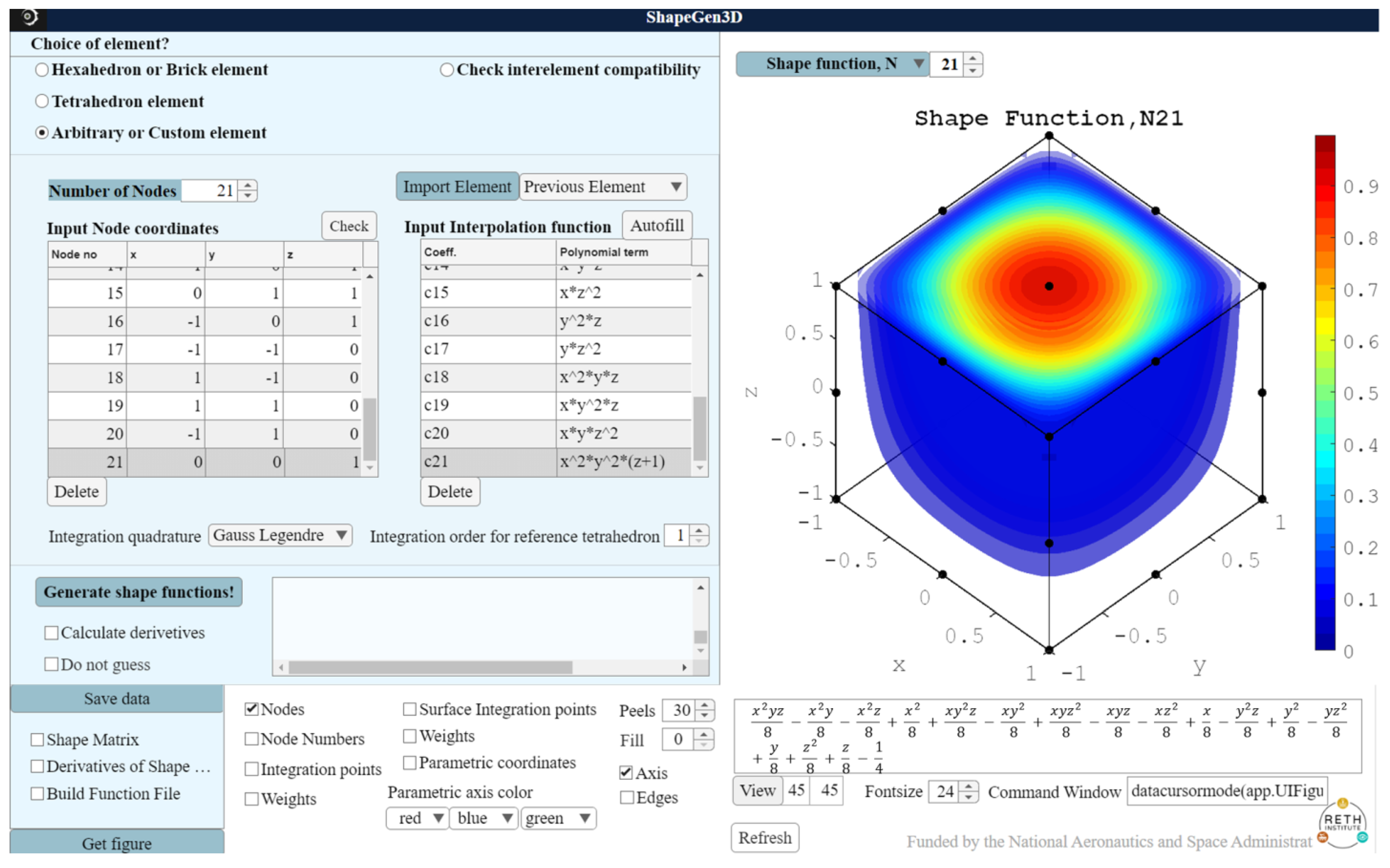
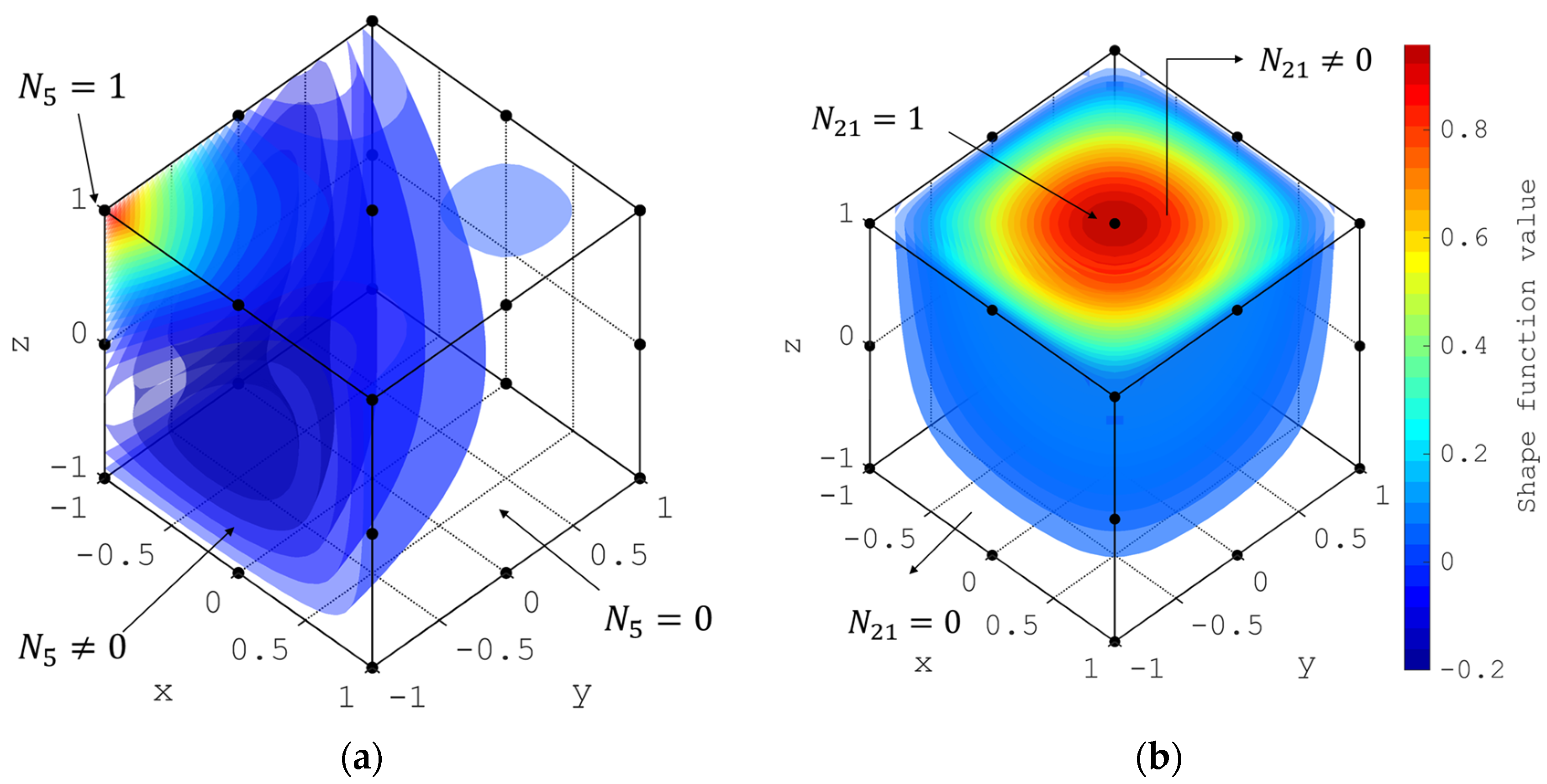
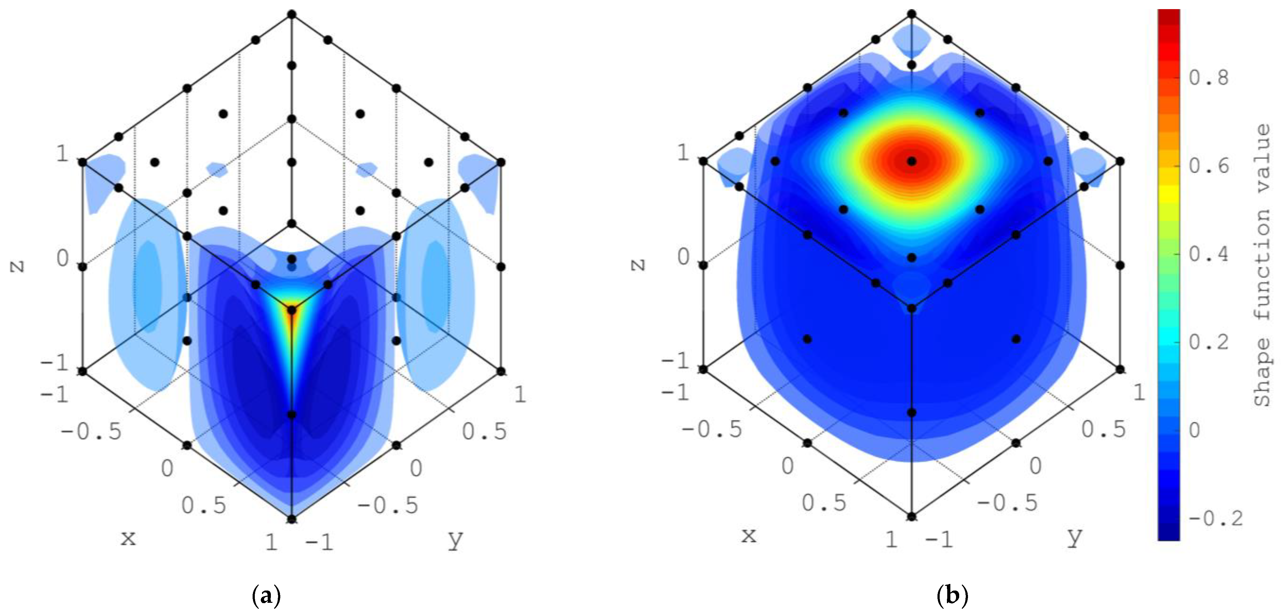
3.2. 21-Node Brick Element

Next, the 21-node brick element was formulated to illustrate the development of a custom element. For this example, the node coordinates and the interpolation function generated for the 20-node element were imported to “Arbitrary or Custom element” by pressing the “Import previous element” button. Then, one node was added manually with coordinate (0,0,−1), and several trials for adding a polynomial term associated with coefficient $c_{21}$ were made until an invertible $\mathit{F}$ matrix (Equation (5)) was obtained by the software. The additional polynomial basis that was added to the interpolation function was $x^2{y}^2(z+1)$, which yields $2x^2{y}^2$ at the $z=1$ surface that contains the 21st mid-surface node and vanishes at the $z=-1$ surface without a mid-surface node. The interpolation function is presented in Equation (53) as,

$$\begin{array}{cc}\hfill f_n=c_1+c_{2}x& +c_{3}y+c_{4}z+c_{5}xy+c_{6}yz+c_{7}xz+c_8{x}^2+c_9{y}^2+c_{10}{z}^2+c_{11}xyz+c_{12}{x}^{2}y\hfill \\ & +c_{13}{x}^{2}z+c_{14}{y}^{2}x+c_{15}{y}^{2}z+c_{16}{z}^{2}x+c_{17}{z}^{2}y+c_{18}{x}^{2}yz+c_{19}x{y}^{2}z+c_{20}xy{z}^2\hfill \\ & +c_{21}{x}^2{y}^2(z+1)\hfill \end{array}$$

(53)

The input to ShapeGen3D is presented in Figure 11, which shows the input coordinate of the 21st node and the polynomial term with coefficient $c_{21}$. The obtained nodal coordinates, corresponding shape functions, and nodes on the surface and surface normal vector pointing outward of the domain for all surfaces are presented in

Table A6. Node_Coordinates for 21 node brick element.

Node Number	x	y	z
1	−1	−1	−1
2	1	−1	−1
3	1	1	−1
4	−1	1	−1
5	−1	−1	1
6	1	−1	1
7	1	1	1
8	−1	1	1
9	0	−1	−1
10	1	0	−1
11	0	1	−1
12	−1	0	−1
13	0	−1	1
14	1	0	1
15	0	1	1
16	−1	0	1
17	−1	−1	0
18	1	−1	0
19	1	1	0
20	−1	1	0
21	0	0	1

,

Table A7. Shape_Functions for 21-node brick element.

Node	${\mathit{N}}_{\mathit{i}}(\mathit{x},\mathit{y},\mathit{z})$
1	$\frac{x^{2}yz}{8}-\frac{x^{2}y}{8}-\frac{x^{2}z}{8}+\frac{x^2}{8}+\frac{x{y}^{2}z}{8}-\frac{x{y}^2}{8}+\frac{xy{z}^2}{8}-\frac{xyz}{8}-\frac{x{z}^2}{8}+\frac{x}{8}-\frac{y^{2}z}{8}+\frac{y^2}{8}-\frac{y{z}^2}{8}+\frac{y}{8}+\frac{z^2}{8}+\frac{z}{8}-\frac{1}{4}$
2	$\frac{x^{2}yz}{8}-\frac{x^{2}y}{8}-\frac{x^{2}z}{8}+\frac{x^2}{8}-\frac{x{y}^{2}z}{8}+\frac{x{y}^2}{8}-\frac{xy{z}^2}{8}+\frac{xyz}{8}+\frac{x{z}^2}{8}-\frac{x}{8}-\frac{y^{2}z}{8}+\frac{y^2}{8}-\frac{y{z}^2}{8}+\frac{y}{8}+\frac{z^2}{8}+\frac{z}{8}-\frac{1}{4}$
3	$-\frac{x^{2}yz}{8}+\frac{x^{2}y}{8}-\frac{x^{2}z}{8}+\frac{x^2}{8}-\frac{x{y}^{2}z}{8}+\frac{x{y}^2}{8}+\frac{xy{z}^2}{8}-\frac{xyz}{8}+\frac{x{z}^2}{8}-\frac{x}{8}-\frac{y^{2}z}{8}+\frac{y^2}{8}+\frac{y{z}^2}{8}-\frac{y}{8}+\frac{z^2}{8}+\frac{z}{8}-\frac{1}{4}$
4	$-\frac{x^{2}yz}{8}+\frac{x^{2}y}{8}-\frac{x^{2}z}{8}+\frac{x^2}{8}+\frac{x{y}^{2}z}{8}-\frac{x{y}^2}{8}-\frac{xy{z}^2}{8}+\frac{xyz}{8}-\frac{x{z}^2}{8}+\frac{x}{8}-\frac{y^{2}z}{8}+\frac{y^2}{8}+\frac{y{z}^2}{8}-\frac{y}{8}+\frac{z^2}{8}+\frac{z}{8}-\frac{1}{4}$
5	$\frac{x}{8}+\frac{y}{8}-\frac{x{y}^2}{8}-\frac{x^{2}y}{8}-\frac{x{z}^2}{8}-\frac{y{z}^2}{8}+\frac{z^2}{8}+\frac{xy{z}^2}{8}-\frac{x{y}^{2}z}{8}-\frac{x^{2}yz}{8}+\frac{xyz}{8}+\frac{x^2{y}^2\left(z+1\right)}{8}-\frac{1}{8}$
6	$\frac{y}{8}-\frac{x}{8}+\frac{x{y}^2}{8}-\frac{x^{2}y}{8}+\frac{x{z}^2}{8}-\frac{y{z}^2}{8}+\frac{z^2}{8}-\frac{xy{z}^2}{8}+\frac{x{y}^{2}z}{8}-\frac{x^{2}yz}{8}-\frac{xyz}{8}+\frac{x^2{y}^2\left(z+1\right)}{8}-\frac{1}{8}$
7	$\frac{x{y}^2}{8}-\frac{y}{8}-\frac{x}{8}+\frac{x^{2}y}{8}+\frac{x{z}^2}{8}+\frac{y{z}^2}{8}+\frac{z^2}{8}+\frac{xy{z}^2}{8}+\frac{x{y}^{2}z}{8}+\frac{x^{2}yz}{8}+\frac{xyz}{8}+\frac{x^2{y}^2\left(z+1\right)}{8}-\frac{1}{8}$
8	$\frac{x}{8}-\frac{y}{8}-\frac{x{y}^2}{8}+\frac{x^{2}y}{8}-\frac{x{z}^2}{8}+\frac{y{z}^2}{8}+\frac{z^2}{8}-\frac{xy{z}^2}{8}-\frac{x{y}^{2}z}{8}+\frac{x^{2}yz}{8}-\frac{xyz}{8}+\frac{x^2{y}^2\left(z+1\right)}{8}-\frac{1}{8}$
9	$\frac{yz}{4}-\frac{z}{4}-\frac{y}{4}+\frac{x^{2}y}{4}+\frac{x^{2}z}{4}-\frac{x^2}{4}-\frac{x^{2}yz}{4}+\frac{1}{4}$
10	$\frac{x}{4}-\frac{z}{4}-\frac{xz}{4}-\frac{x{y}^2}{4}+\frac{y^{2}z}{4}-\frac{y^2}{4}+\frac{x{y}^{2}z}{4}+\frac{1}{4}$
11	$\frac{y}{4}-\frac{z}{4}-\frac{yz}{4}-\frac{x^{2}y}{4}+\frac{x^{2}z}{4}-\frac{x^2}{4}+\frac{x^{2}yz}{4}+\frac{1}{4}$
12	$\frac{xz}{4}-\frac{z}{4}-\frac{x}{4}+\frac{x{y}^2}{4}+\frac{y^{2}z}{4}-\frac{y^2}{4}-\frac{x{y}^{2}z}{4}+\frac{1}{4}$
13	$\frac{x^{2}y}{4}-\frac{yz}{4}-\frac{y}{4}+\frac{y^{2}z}{4}+\frac{y^2}{4}+\frac{x^{2}yz}{4}-\frac{x^2{y}^2\left(z+1\right)}{4}$
14	$\frac{x}{4}+\frac{xz}{4}-\frac{x{y}^2}{4}+\frac{x^{2}z}{4}+\frac{x^2}{4}-\frac{x{y}^{2}z}{4}-\frac{x^2{y}^2\left(z+1\right)}{4}$
15	$\frac{y}{4}+\frac{yz}{4}-\frac{x^{2}y}{4}+\frac{y^{2}z}{4}+\frac{y^2}{4}-\frac{x^{2}yz}{4}-\frac{x^2{y}^2\left(z+1\right)}{4}$
16	$\frac{x{y}^2}{4}-\frac{xz}{4}-\frac{x}{4}+\frac{x^{2}z}{4}+\frac{x^2}{4}+\frac{x{y}^{2}z}{4}-\frac{x^2{y}^2\left(z+1\right)}{4}$
17	$\frac{xy}{4}-\frac{y}{4}-\frac{x}{4}+\frac{x{z}^2}{4}+\frac{y{z}^2}{4}-\frac{z^2}{4}-\frac{xy{z}^2}{4}+\frac{1}{4}$
18	$\frac{x}{4}-\frac{y}{4}-\frac{xy}{4}-\frac{x{z}^2}{4}+\frac{y{z}^2}{4}-\frac{z^2}{4}+\frac{xy{z}^2}{4}+\frac{1}{4}$
19	$\frac{x}{4}+\frac{y}{4}+\frac{xy}{4}-\frac{x{z}^2}{4}-\frac{y{z}^2}{4}-\frac{z^2}{4}-\frac{xy{z}^2}{4}+\frac{1}{4}$
20	$\frac{y}{4}-\frac{x}{4}-\frac{xy}{4}+\frac{x{z}^2}{4}-\frac{y{z}^2}{4}-\frac{z^2}{4}+\frac{xy{z}^2}{4}+\frac{1}{4}$
21	$\frac{z}{2}-\frac{x^{2}z}{2}-\frac{y^{2}z}{2}-\frac{x^2}{2}-\frac{y^2}{2}+\frac{x^2{y}^2\left(z+1\right)}{2}+\frac{1}{2}$

and

Table A8. Surface_Nodes_and_vectors for 21-node brick element.

Node Number	${\mathit{n}}_{\mathit{x}}$	${\mathit{n}}_{\mathit{y}}$	${\mathit{n}}_{\mathit{z}}$
2	1	0	0
3	1	0	0
6	1	0	0
7	1	0	0
10	1	0	0
14	1	0	0
18	1	0	0
19	1	0	0
1	−1	0	0
4	−1	0	0
5	−1	0	0
8	−1	0	0
12	−1	0	0
16	−1	0	0
17	−1	0	0
20	−1	0	0
3	0	1	0
4	0	1	0
7	0	1	0
8	0	1	0
11	0	1	0
15	0	1	0
19	0	1	0
20	0	1	0
1	0	−1	0
2	0	−1	0
5	0	−1	0
6	0	−1	0
9	0	−1	0
13	0	−1	0
17	0	−1	0
18	0	−1	0
5	0	0	1
6	0	0	1
7	0	0	1
8	0	0	1
13	0	0	1
14	0	0	1
15	0	0	1
16	0	0	1
21	0	0	1
1	0	0	−1
2	0	0	−1
3	0	0	−1
4	0	0	−1
9	0	0	−1
10	0	0	−1
11	0	0	−1
12	0	0	−1

, respectively. Other element variables, such as integration points and weights, match those of the 20-node brick element shown in Table A8.

For stage 3, each shape function can be analyzed to check the accuracy of the calculations performed by the software. The element must satisfy two conditions: (1) the interpolation condition; and (2) local support. As stated in Section 2, the interpolation condition was satisfied when an invertible matrix F of Equation (5) was obtained. The graphical illustrations of each shape function can be used to check if the local support condition is satisfied. For example, Figure 12 plots shape functions at nodes 5 and 21, $N_5$ and $N_{21}$, where the shape functions are shown to vanish at the face that does not contain the nodes, and thus, satisfying the local support condition.

Next, on stage 4, the compatibility with the 20-node brick element was checked. For this purpose, the “Check compatibility” button was selected. Figure 13 shows the results of the intercompatibility check of the first surface pair between the two elements, which was performed according to the procedure described in Section 2.5. The green lamp next to the compatibility text in Figure 10 indicates that the interelement compatibility condition was satisfied. A red lamp would indicate that the intercompatibility condition was not met. This condition can also be verified qualitatively using the plots of shape functions corresponding to the connecting nodes, which show the same shape function profile at the element boundary. By checking all of the surface pairs, it is concluded that any surface can be the interelement surface between the 20 and 21-node elements, except the $xy$ face at $z=1$.

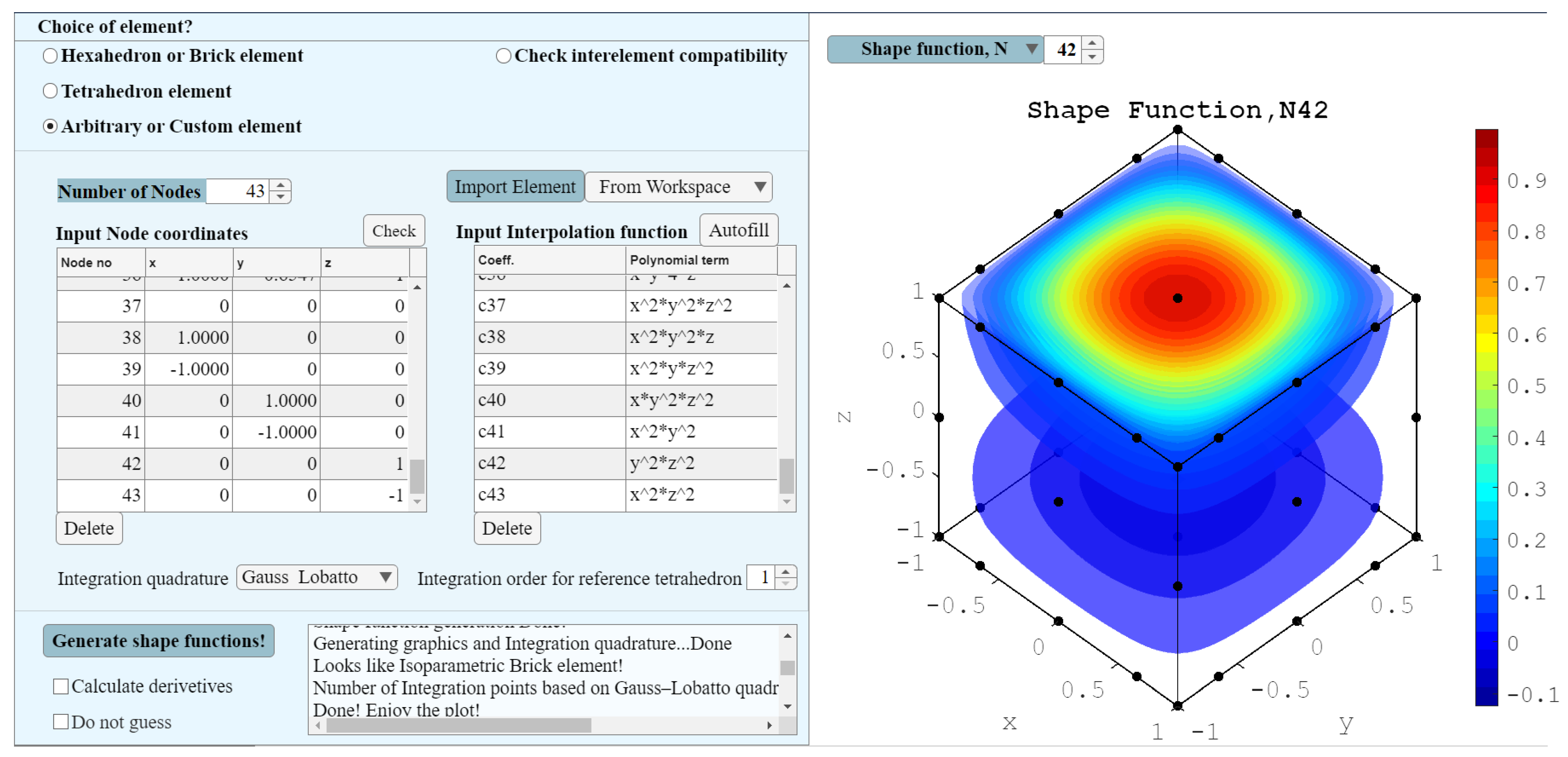
3.3. 43-Node Hexahedron Element

A 43-node hexahedron element was formulated following a similar procedure as the 21-node, such that the interpolation function provided a solution to the plate bending equation. According to the Kirchhoff–Love plate theory [41] for isotropic plates, the displacement along the z-axis, $w$, follows the differential equation as,

$$\frac{2\rho h}{D}\frac{{\partial }^{2}w}{\partial t^2}+\left(\frac{{\partial }^{4}w}{\partial x^4}+2\frac{{\partial }^{4}w}{\partial x^2\partial y^2}+\frac{{\partial }^{4}w}{\partial y^4}\right)=\frac{q}{D}$$

(54)

where $q$ is the constant distributed load, and $D$ is the flexure rigidity. If the time derivative is canceled, it forms the Germain–Lagrange plate equation. A polynomial solution of this differential equation can be written as,

$$\begin{array}{cc}\hfill w_n=c_1+c_{2}x& +c_{3}y+c_4{x}^2+c_{5}xy+c_6{y}^2+c_7{x}^3+c_8{x}^2+c_{9}y{x}^2+c_{10}x{y}^2+c_{11}{y}^3+c_{12}{x}^4\hfill \\ & +c_{13}{x}^{3}y+c_{14}x{y}^3+c_{15}{y}^4+c_{16}{x}^2{y}^2\hfill \end{array}$$

(55)

A 3D element was formulated keeping the lowest order as quadratic along the z-axis such that the interpolation function contained the polynomial basis presented in Equation (55). First, a 36-node hexahedron element of the Serendipity family was formulated with the options $m_x=4$, $m_y=4$ and $m_z=2$. This interpolation function of this Serendipity element does not contain the $x^2{y}^2$ term, hence, it cannot replicate the solution of Equation (54) exactly. Thus, the element was imported as an arbitrary element, and seven additional nodes with coordinates ($\pm 1,0,0$), ($0,\pm 1,0$), ($0,0,\pm 1$), and ($0,0,0$) were added. Finally, seven polynomial basis as $x^2{y}^2{z}^2$, $x^2{y}^{2}z$, $x^{2}y{z}^2,x{y}^2{z}^2,x^2{y}^2,z^2{y}^2$ and $x^2{z}^2$ were added to formulate the 43-node element that has the polynomial interpolation function as presented in Equation (56). The screenshot of this element formulation is presented in Figure 14.

$$\begin{array}{cc}\hfill f_n=c_1+c_{2}x& +c_{3}y+c_{4}z+c_5{x}^2+c_{6}xy+c_{7}xz+c_8{y}^2+c_{9}yz+c_{10}{z}^2\hfill \\ & +c_{11}{x}^3+c_{12}{x}^{2}y+c_{13}{x}^{2}z+c_{15}x{y}^2+c_{16}xyz+c_{17}x{z}^2+c_{18}{y}^3\hfill \\ & +c_{19}{y}^{2}z+c_{20}y{z}^2+c_{21}{x}^4+c_{22}{x}^{3}y+c_{23}{x}^{3}z+c_{24}{x}^{2}yz+c_{25}x{y}^3\hfill \\ & +c_{26}x{y}^{2}z+c_{27}xy{z}^2+c_{28}{y}^4+c_{29}{y}^{3}z+c_{30}{x}^{4}y+c_{31}{x}^{4}z\hfill \\ & +c_{32}{x}^{3}yz+c_{33}x{y}^4+c_{34}x{y}^{3}z+c_{35}{y}^{4}z+c_{36}{x}^{4}yz+c_{37}x{y}^{4}z\hfill \\ & +c_{38}{x}^2{y}^2{z}^2+c_{39}{x}^2{y}^{2}z+c_{40}{x}^{2}y{z}^2+c_{41}x{y}^2{z}^2+c_{42}{x}^2{y}^2\hfill \\ & +c_{43}{y}^2{z}^2,x^2{z}^2\hfill \end{array}$$

(56)

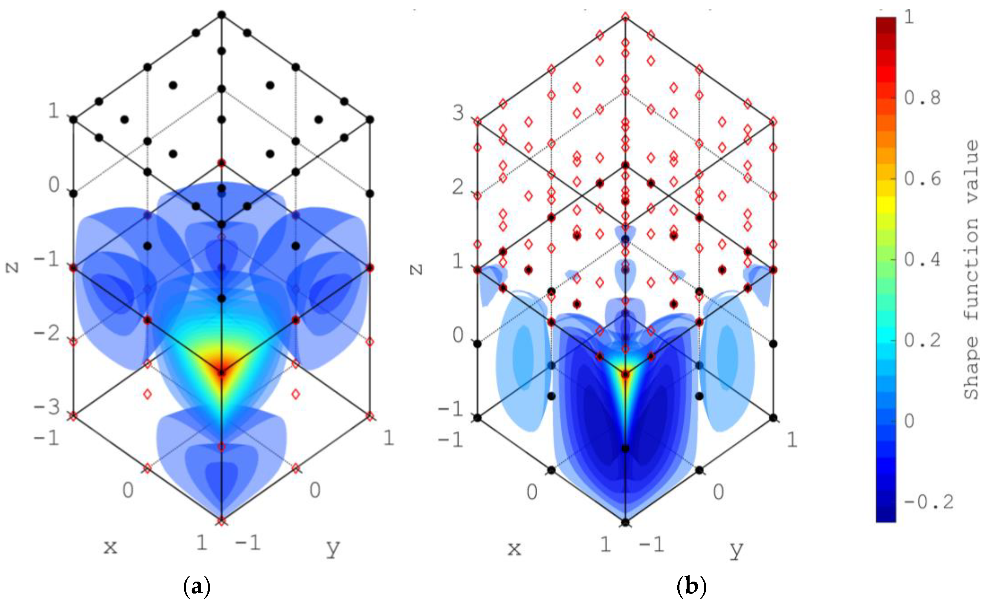
3.4. 43-Node Transition Element from Fourth to Second-Order Lagrangian Element

The fourth-order Lagrangian element is a 125-node element $(m_x=m_y=m_z=4)$ with five nodes along each axis. Such high-order elements can replicate wave propagation and are widely used in the structural health monitoring field [13,14,15,16]. The second-order Lagrangian element is a 27-node element ($m_x=m_y=m_z=2)$ with three nodes along each axis. In this example, a transition element was developed to bridge these two elements. The transition element is considered to be of second order along the $z$-axis.

The $z=1$ surface of the transition element should match the $z=\mp 1$ surface of the 125-node element, and $z=-1$ surface should match the 27-node element’s surface. Hence, there will be 25 nodes on the $z=1$ surface and nine nodes on the $z=-1$ surface. As the order of the transition element is two, instead of a 125-node element, a 75-node element with $m_x=m_y=4$ and $m_z=2$ was considered as the reference element. Upon formulation of the 75-node element, the nodes at the $z=-1$ surface are removed to replicate the surface of a 27-node element.

The minimum order of the element is 2. Hence, all the monomial basis functions of order 2 are kept. As the element needs to transition from order 4 to 2 along the $z$-axis, the monomial basis that has order $m_z=1$ was kept and manipulated as $\left(z+1\right)$, such that those terms vanish at the $z=-1$ surface, as presented in

Table 5. Factors of interpolation function of 75 and 43 node elements.

Coefficient No.	75 Node Element Factors	43 Node Element Factors
Factors with, $$\begin{gathered} m_x<3 \\ {m}_y<3 \\ {m}_z<3 \end{gathered}$$	Factors of $f_{n20}$	Factors of $f_{n20}$
	$x^2{y}^2$	$x^2{y}^2$
	$x^2{y}^{2}z$	$x^2{y}^{2}z$
	$x^{2}y{z}^2$	$x^{2}y{z}^2$
	$x{y}^2{z}^2$	$x{y}^2{z}^2$
	$x^2{y}^2{z}^2$	$x^2{y}^2{z}^2$
	$x^2{z}^2$	$x^2{z}^2$
	$y^2{z}^2$	$y^2{z}^2$
Factors with $m_z=1$	$x^{3}z$	$x^3\left(z+1\right)$
	$y^{3}z$	$y^3\left(z+1\right)$
	$x^{4}z$	$x^4\left(z+1\right)$
	$x^{3}yz$	$x^{3}y\left(z+1\right)$
	$y^{3}z$	$y^3\left(z+1\right)$
	$y^{4}z$	$y^4\left(z+1\right)$
	$x^{4}yz$	$x^{4}y\left(z+1\right)$
	$x^3{y}^{2}z$	$x^3{y}^2\left(z+1\right)$
	$x^2{y}^{3}z$	$x^2{y}^3\left(z+1\right)$
	$x{y}^{4}z$	$x{y}^4\left(z+1\right)$
	$x^4{y}^{2}z$	$x^4{y}^2\left(z+1\right)$
	$x^2{y}^{4}z$	$x^2{y}^4\left(z+1\right)$
	$x^4{y}^{3}z$	$x^4{y}^3\left(z+1\right)$
	$x^3{y}^{4}z$	$x^3{y}^4\left(z+1\right)$
	$x^3{y}^{3}z$	$x^3{y}^3\left(z+1\right)$
	$x^4{y}^{4}z$	$x^4{y}^4\left(z+1\right)$

. The remaining 43 terms form the interpolation function of the 43-node transition element.

The generated element satisfies the local support conditions presented in Figure 15 for two shape functions, nodes 6 and 35. The inter-element compatibility conditions were also checked, and compatibility was observed between the $z=1$ surface of the transition element and the fourth-order element and between the $z=-1$ surface of the transition and the second-order element. Figure 16 presents a graphical overview of the compatibility check. The red hollow diamond represents the nodes of the second-order (Figure 16a) and fourth-order (Figure 16b) elements, whereas the black dots represent the transition element. It is evident that the node coordinates match, and the shape functions agree at the common nodes.

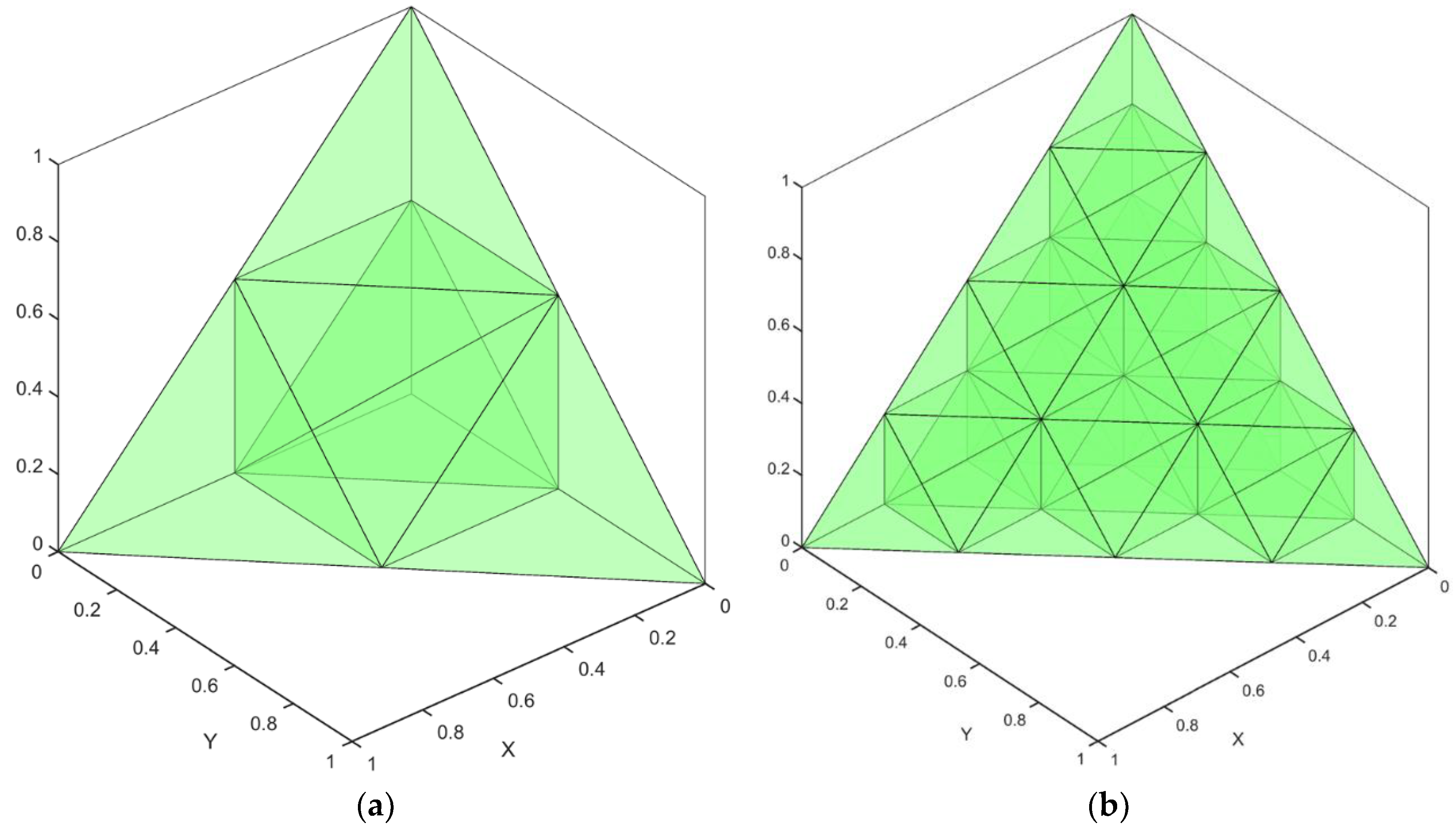
3.5. Spectral Elements

Finally, the shape functions were generated for a hexahedron element of the Lagrangian family with 108 nodes to provide a complete overview of the methodology. In ShapeGen3D, $m_x=5$, $m_y=5$, and $m_z=2$ were provided as input parameters. The shape function for node 70 of the element is presented in Figure 17a. The red spot of the plot indicates the location of this node. It can be observed that the shape function satisfies the interpolation and local support conditions as it vanishes to 0 over surfaces that do not contain the node. The same behavior is observed for other nodes. This spectral element was used for simulating guided waves by Soman et al. [15].

Additionally, a 5th-order tetrahedron element (56 nodes) with input $m=5$ (Equation (13)) was formulated. The shape function for the 50th node of the element is presented in Figure 17b. All shape functions for this element were also observed to satisfy the interpolation and local support conditions. Thus, analysts using the spectral finite element method can use ShapeGen3D to determine the formulation for arbitrary noded elements.

4. Discussion

This development reduces implementation effort in formulating and verifying arbitrary 3D elements for FEM applications. It provides FEM users the possibility to employ elements beyond those available in commercial FEM software, FEM libraries, and open-access codes. The proposed procedure facilitates the formulation of higher-order elements, which can be shown to solve challenging problems with fewer degrees of freedom in some applications. The software was developed as part of a NASA-sponsored space technology research institute, Resilient Extra-Terrestrial Habitat Institute (RETHi), which aims to propel space exploration forward by developing new knowledge, technologies, and techniques. ShapeGen3D was used to develop the 21-node brick elements presented in this paper to capture meteoroid impact loading on a space habitat model. The model was embedded within a Modular coupled virtual testbed (MCVT) [42,43] that integrates several sub-systems of a space habitat to evaluate their interdependence and the effectiveness of safety controls when a habitat is exposed to external disturbances. ShapeGen3D allowed developers to easily adjust the elements of the structural model until the functional requirements were met. A 43-node brick element was also developed with ShapeGen3D to mimic wave propagation due to meteoroid impact and assist with generating a structural health monitoring algorithm for detecting damage.

Upon publication, this development is expected to benefit the computational mechanics community beyond the RETHi group. The higher-order and transition element formulation that the software can generate will allow researchers to employ elements that can increase the accuracy and reduce the computational time when dealing with simulations that involve contact, mesh transition regions, and Lagrangian solid dynamics. Furthermore, ShapeGen3D can become an educational tool to illustrate three-dimensional FEM concepts.

5. Conclusions

This work presents the development of a generalized procedure for formulating nodal coordinates, shape functions, and integration quadrature of higher-order hexahedrons, tetrahedrons, and arbitrary or custom elements in 3D. This procedure also derived expressions for checking the interelement compatibility of adjacent elements, which enables incorporating newly formulated elements within multielement meshes. The procedure was incorporated into GUI software, ShapeGen3D, to facilitate its implementation. In this paper, several elements were formulated to verify the accuracy of the implementation. ShapeGen3D allows users to verify that the nodal shape conditions are met and checks the element’s compatibility with other elements through a graphical interface. This advanced feature was illustrated through the 21-hexahedron element, where compatibility with a 20-node brick element was checked. Additionally, 43-node elements were formulated to capture the behavior of a Germain–Lagrange plate and establish a transition between Lagrangian elements of different order. Finally, a fifth-order tetrahedron element was generated to simulate guided waves. Thus, this work can have potential impacts on the accuracy and efficiency of FEM runs, as it can be used to generate elements that minimize the number of elements and degrees of freedoms used in traditional analyses, develop transition elements that connect fine to coarse mesh regions, and generate high-order spectral elements that accurately capture waves propagating through solid bodies. The numerical results illustrate that the generalized procedure captured in ShapeGen3D can significantly benefit research and development in FEM and numerical methods.

References

1. Zienkiewicz, O.C.; Taylor, R.L.; Zhu, J.Z. The Finite Element Method: Its Basis and Fundamentals, 7th ed.; Elsevier: Amsterdam, The Netherlands, 2013. [Google Scholar] [CrossRef]
2. Bunting, C.F. Introduction to the finite element method. In Proceedings of the 2008 IEEE International Symposium on Electromagnetic Compatibility, Detroit, MI, USA, 18–22 August 2008; pp. 1–9. [Google Scholar] [CrossRef]
3. Chari, M.; Salon, S. Numerical Methods in Electromagnetism; Elsevier: Amsterdam, The Netherlands, 2000. [Google Scholar] [CrossRef]
4. Bathe, K.-J. Discontinuous Finite Element Procedures. In Computational Fluid and Solid Mechanics; Springer: London, UK, 2006; pp. 21–43. [Google Scholar] [CrossRef]
5. Logg, A.; Lundholm, C.; Nordaas, M. Finite element simulation of physical systems in augmented reality. Adv. Eng. Softw. 2020, 149, 102902. [Google Scholar] [CrossRef]
6. Liu, L.; Davies, K.B.; Křížek, M.; Guan, L. On Higher Order Pyramidal Finite Elements. Adv. Appl. Math. Mech. 2011, 3, 131–140. [Google Scholar] [CrossRef]
7. Smith, M. ABAQUS/Standard User’s Manual, Version 6.9; Dassault Systèmes Simulia Corp.: Johnston, RI, USA, 2009. [Google Scholar]
8. Staten, M.L.; Jones, N.L. Local refinement of three-dimensional finite element meshes. Eng. Comput. 1997, 13, 165–174. [Google Scholar] [CrossRef]
9. Duczek, S.; Saputra, A.; Gravenkamp, H. High order transition elements: The xy-element concept—Part I: Statics. Comput. Methods Appl. Mech. Eng. 2020, 362, 112833. [Google Scholar] [CrossRef]
10. Buczkowski, R. 21-node hexahedral isoparametric element for analysis of contact problems. Commun. Numer. Methods Eng. 1998, 14, 681–692. [Google Scholar] [CrossRef]
11. Smith, I.M.; Kidger, D.J. Elastoplastic analysis using the 14-node brick element family. Int. J. Numer. Methods Eng. 1992, 35, 1263–1275. [Google Scholar] [CrossRef]
12. Canuto, C.; Hussaini, M.Y.; Quarteroni, A.; Zang, T.A. Spectral Approximation. In Spectral Methods in Fluid Dynamics; Springer: Berlin/Heidelberg, Germany, 1988; pp. 31–75. [Google Scholar] [CrossRef]
13. Patera, A.T. A spectral element method for fluid dynamics: Laminar flow in a channel expansion. J. Comput. Phys. 1984, 54, 468–488. [Google Scholar] [CrossRef]
14. Palacz, M.; Krawczuk, M.; Żak, A. Spectral Element Methods for Damage Detection and Condition Monitoring. In Smart Innovation, Systems and Technologies; Springer: Berlin/Heidelberg, Germany, 2020; Volume 166, pp. 549–558. [Google Scholar] [CrossRef]
15. Soman, R.; Kudela, P.; Balasubramaniam, K.; Singh, S.K.; Malinowski, P. A Study of Sensor Placement Optimization Problem for Guided Wave-Based Damage Detection. Sensors 2019, 19, 1856. [Google Scholar] [CrossRef]
16. Ostachowicz, W.; Kudela, P.; Krawczuk, M.; Zak, A. Guided Waves in Structures for SHM: The Time-Domain Spectral Element Method; John Wiley & Sons, Ltd.: New York, NY, USA, 2012. [Google Scholar] [CrossRef]
17. Komatitsch, D.; Tromp, J. Spectral-element simulations of global seismic wave propagation-I. Validation. Geophys. J. Int. 2002, 149, 390–412. [Google Scholar] [CrossRef]
18. Arnold, D.N.; Awanou, G. The Serendipity Family of Finite Elements. Found. Comput. Math. 2011, 11, 337–344. [Google Scholar] [CrossRef]
19. Silvester, P. Tetrahedral polynomial finite elements for the Helmholtz equation. Int. J. Numer. Methods Eng. 1972, 4, 405–413. [Google Scholar] [CrossRef]
20. Duczek, S.; Duvigneau, F.; Gabbert, U. The finite cell method for tetrahedral meshes. Finite Elem. Anal. Des. 2016, 121, 18–32. [Google Scholar] [CrossRef]
21. Kabir, H.; Matikolaei, S.A.H.H. Implementing an accurate generalized gaussian quadrature solution to find the elastic field in a homogeneous anisotropic media. J. Serbian Soc. Comput. Mech. 2017, 11, 11–19. [Google Scholar] [CrossRef]
22. von Winckel, G. Legende-Gauss-Lobatto Nodes and Weights. MATLAB Central File Exchange. Available online: https://www.mathworks.com/matlabcentral/fileexchange/4775-legende-gauss-lobatto-nodes-and-weights (accessed on 20 September 2023).
23. Sherwin, S.J.; Karniadakis, G.E. A new triangular and tetrahedral basis for high-order (hp) finite element methods. Int. J. Numer. Methods Eng. 1995, 38, 3775–3802. [Google Scholar] [CrossRef]
24. Moore, J.L.; Morgan, N.R.; Horstemeyer, M.F. ELEMENTS: A high-order finite element library in C++. SoftwareX 2019, 10, 100257. [Google Scholar] [CrossRef]
25. Cantwell, C.D.; Moxey, D.; Comerford, A.; Bolis, A.; Rocco, G.; Mengaldo, G. Nektar++: An open-source spectral/hp element framework. Comput. Phys. Commun. 2015, 192, 205–219. [Google Scholar] [CrossRef]
26. Vishwanatha, J.S.; Swamy, R.H.M.S.; Mahesh, G.; Gouda, H.V. A toolkit for computational fluid dynamics using spectral element method in Scilab. Mater. Today Proc. 2023. [Google Scholar] [CrossRef]
27. Bangerth, W.; Hartmann, R.; Kanschat, G. deal. II—a general-purpose object-oriented finite element library. ACM Trans. Math. Softw. 2007, 33, 24. [Google Scholar] [CrossRef]
28. Bastian, P.; Blatt, M.; Dedner, A.; Engwer, C.; Klöfkorn, R.; Kornhuber, R.; Ohlberger, M.; Sander, O. A generic grid interface for parallel and adaptive scientific computing. Part II: Implementation and tests in DUNE. Computing 2008, 82, 121–138. [Google Scholar] [CrossRef]
29. Kolev, T. Modular Finite Element Methods; No. MFEM; Lawrence Livermore National Lab. (LLNL): Livermore, CA, USA, 2020.
30. Weng, W.-C. Web-based post-processing visualization system for finite element analysis. Adv. Eng. Softw. 2011, 42, 398–407. [Google Scholar] [CrossRef]
31. Beneš, Š.; Kruis, J. Efficient methods to visualize finite element meshes. Adv. Eng. Softw. 2015, 79, 81–90. [Google Scholar] [CrossRef]
32. Wachspress, E.L. A Rational Basis for Function Approximation. IMA J. Appl. Math. 1973, 11, 83–104. [Google Scholar] [CrossRef]
33. Kien, D.N.; Zhuang, X. Radial basis function based finite element method: Formulation and applications. Eng. Anal. Bound. Elem. 2023, 152, 455–472. [Google Scholar] [CrossRef]
34. Parvizian, J.; Düster, A.; Rank, E. Finite cell method. Comput. Mech. 2007, 41, 121–133. [Google Scholar] [CrossRef]
35. Schillinger, D.; Kollmannsberger, S.; Mundani, R.-P.; Rank, E. The finite cell method for geometrically nonlinear problems of solid mechanics. In IOP Conference Series: Materials Science and Engineering; Elsevier: Amsterdam, The Netherlands, 2014; Volume 10, pp. 3768–3782. [Google Scholar] [CrossRef]
36. Fortune, S. Voronoi diagrams and delaunay triangulations. In Handbook of Discrete and Computational Geometry, 3rd ed.; World Scientific: Singapore, 2017; pp. 705–721. [Google Scholar] [CrossRef]
37. Maździarz, M. Unified isoparametric 3D lagrangeFinite elements. CMES—Comput. Model. Eng. Sci. 2010, 66, 1–24. [Google Scholar]
38. Neto, M.A.; Amaro, A.; Roseiro, L.; Cirne, J.; Leal, R. Engineering Computation of Structures: The Finite Element Method; Springer: Berlin/Heidelberg, Germany, 2015. [Google Scholar] [CrossRef]
39. Bourbaki, N. Algebra I: Chapters 1–3; Springer Science & Business Media: Berlin/Heidelberg, Germany, 1998; Volume 1. [Google Scholar]
40. Luo, H.; Pozrikidis, C. A Lobatto interpolation grid in the tetrahedron. IMA J. Appl. Math. 2006, 71, 298–313. [Google Scholar] [CrossRef]
41. Reddy, J.N. Theory and Analysis of Elastic Plates and Shells, 2nd ed.; Taylor and Francis Group: Abingdon, UK, 2006. [Google Scholar]
42. Shahriar, A.; Reynolds, S.; Najarian, M.; Montoya, A. Development of a Computational Framework for the Design of Resilient Space Structures. Earth and Space 2021: Space Exploration, Utilization, Engineering, and Construction in Extreme Environments. In Proceedings of the 17th Biennial International Conference on Engineering, Science, Construction, and Operations in Challenging Environments, Online, 19–23 April 2021; pp. 1263–1271. [Google Scholar] [CrossRef]
43. Kitching, R.; Mattingly, H.; Williams, D.; Marais, K. Resilient Space Habitat Design Using Safety Controls. Earth and Space 2021: Space Exploration, Utilization, Engineering, and Construction in Extreme Environments. In Proceedings of the 17th Biennial International Conference on Engineering, Science, Construction, and Operations in Challenging Environments, Online, 19–23 April 2021; pp. 992–1003. [Google Scholar] [CrossRef]
Figure 1. Element formulation procedure flowchart.
Computation 11 00197 g001
Figure 2. Compatibility condition check flowchart (Stage 3).
Computation 11 00197 g002
Figure 3. Algorithm for shape function determination.
Computation 11 00197 g003
Figure 4. Decomposition of the reference tetrahedron, (a) 8, (b) 64.
Computation 11 00197 g004
Figure 5. Elements 1 (a) and 2 (b) in x coordinate. Bold black rectangle indicates surface p and q.
Computation 11 00197 g005
Figure 6. Element 2 after transformation in X coordinate.
Computation 11 00197 g006
Figure 7. Delaunay triangulation and mapping.
Computation 11 00197 g007
Figure 8. Software overview.
Computation 11 00197 g008
Figure 9. Overview of the options in Segments 1 and 2: (a) Hexahedron or Brick elements, (b) Tetrahedron element, (c) Arbitrary or Custom elements, and (d) Check interelement compatibility.
Computation 11 00197 g009
Figure 10. Input for 20-node brick element.
Computation 11 00197 g010
Figure 11. Input for the 21-node element.
Computation 11 00197 g011
Figure 12. Nodal shape function for (a) Node 5 and (b) Node 21 evaluated in the space of the 21-node hexahedron element.
Computation 11 00197 g012
Figure 13. Shape function comparison between the 20 and 21-node brick elements.
Computation 11 00197 g013
Figure 14. Formulation of 43-node brick element.
Computation 11 00197 g014
Figure 15. Nodal shape function for (a) Node 6 and (b) Node 35.
Computation 11 00197 g015
Figure 16. Inter-element compatibility with (a) quadratic and (b) fourth-order Lagrangian element.
Computation 11 00197 g016
Figure 17. Evaluation of shape functions over the volume of the element for (a) N70 of a higher-order hexahedron and (b) N50 of a higher-order tetrahedron element.
Computation 11 00197 g017