Article

Comparison and Evaluation of Machine Learning-Based Classification of Hand Gestures Captured by Inertial Sensors

1
Faculty of Electrical Engineering, Mechanical Engineering and Naval Architecture—FESB, University of Split, 21000 Split, Croatia
2
Faculty of Mechanical Engineering, Computing and Electrical Engineering, University of Mostar, 88000 Mostar, Bosnia and Herzegovina
*
Author to whom correspondence should be addressed.
Computation 2022, 10(9), 159; https://doi.org/10.3390/computation10090159
Submission received: 26 July 2022 / Revised: 1 September 2022 / Accepted: 8 September 2022 / Published: 14 September 2022
(This article belongs to the Special Issue Applications of Statistics and Machine Learning in Electronics)

Abstract

:
Gesture recognition is a topic in computer science and language technology that aims to interpret human gestures with computer programs and many different algorithms. It can be seen as the way computers can understand human body language. Today, the main interaction tools between computers and humans are still the keyboard and mouse. Gesture recognition can be used as a tool for communication with the machine and interaction without any mechanical device such as a keyboard or mouse. In this paper, we present the results of a comparison of eight different machine learning (ML) classifiers in the task of human hand gesture recognition and classification to explore how to efficiently implement one or more tested ML algorithms on an 8-bit AVR microcontroller for on-line human gesture recognition with the intention to gesturally control the mobile robot. The 8-bit AVR microcontrollers are still widely used in the industry, but due to their lack of computational power and limited memory, it is a challenging task to efficiently implement ML algorithms on them for on-line classification. Gestures were recorded by using inertial sensors, gyroscopes, and accelerometers placed at the wrist and index finger. One thousand and eight hundred (1800) hand gestures were recorded and labelled. Six important features were defined for the identification of nine different hand gestures using eight different machine learning classifiers: Decision Tree (DT), Random Forests (RF), Logistic Regression (LR), Linear Discriminant Analysis (LDA), Support Vector Machine (SVM) with linear kernel, Naïve Bayes classifier (NB), K-Nearest Neighbours (KNN), and Stochastic Gradient Descent (SGD). All tested algorithms were ranged according to Precision, Recall, and F1-score (abb.: P-R-F1). The best algorithms were SVM (P-R-F1: 0.9865, 0.9861, and 0.0863), and RF (P-R-F1: 0.9863, 0.9861, and 0.0862), but their main disadvantage is their unusability for on-line implementations in 8-bit AVR microcontrollers, as proven in the paper. The next best algorithms have had only slightly poorer performance than SVM and RF: KNN (P-R-F1: 0.9835, 0.9833, and 0.9834) and LR (P-R-F1: 0.9810, 0.9810, and 0.9810). Regarding the implementation on 8-bit microcontrollers, KNN has proven to be inadequate, like SVM and RF. However, the analysis for LR has proved that this classifier could be efficiently implemented on targeted microcontrollers. Having in mind its high F1-score (comparable to SVM, RF, and KNN), this leads to the conclusion that the LR is the most suitable classifier among tested for on-line applications in resource-constrained environments, such as embedded devices based on 8-bit AVR microcontrollers, due to its lower computational complexity in comparison with other tested algorithms.

1. Introduction

Nowadays, in a world where computers become more and more pervasive in culture, the need for efficient human–computer interaction is increasing at a rapid pace. The most commonly used way of human–computer interaction (HCI) is a graphical user interface (GUI) which requires the use of additional devices, e.g., mouse, keyboard, etc. Researchers in academia and industry are increasingly looking for ways to make human–computer interaction easier, safer, and more efficient. Consequently, new interaction styles have been explored. One of them is hand gesture-based interaction, which allows users a more natural way to communicate without any extra devices, which is much simpler and more intuitive than using graphical interfaces or text input. For example, such a type of interaction is used in applications like controlling smart interactive televisions [1] or enabling a hand as a 3D mouse. Recognized gestures also can be used for controlling a robot [2] or conveying meaningful information. It can be very useful in particular situations, e.g., with robots designed to assist disabled people and help them with personal and professional tasks daily or for real-time mobile robot control [2].
The key problem in hand gesture-based interaction is how to make gestures easily understandable and accurately interpretable to computers. Thus, hand gesture recognition is an area of active research in the field of computer vision and machine learning. Accordingly, different approaches have been considered and all of them can be mainly divided into two groups: vision-based [3,4] and inertial-sensor-based [2,5,6,7,8,9] methods. Besides vision and inertial-sensor-based methods, some recent studies employ surface electromyography in hand gesture recognition as well [10].
Vision-based hand gesture recognition methods use a camera for the detection and identification of human action and motion for various tasks, such as video search engines [11], and computer interface control using hand gestures [12]. Requiring only a camera is the main advantage of these systems. On the other hand, the major drawbacks are sensitivity to the change in field of view and/or the background, unexpected ambient optical noise, the change in lighting conditions, and relatively intensive data processing. Due to the necessity of hand gesture recognition to be reliable, accurate, and robust for work in real-time, researchers often tend to use methods based on inertial sensors [2,5,6,7,8,9,13]. These methods involve the use of sensors placed on the user’s body.
With the development of small inexpensive sensors, inertial-based techniques became more available and have created new opportunities for novel human–computer interface designs. In gesture recognition, two main popular approaches are available: body-worn systems that track user gestures and motion using body-worn sensors attached to the human body, or external systems based on external sensors. Many gesture recognition studies [14,15,16,17] use sensors like Microsoft Kinect which allows human identification and tracking in 3D spaces using RGB-D sensors which combine RGB colour information with per-pixel depth information to obtain information about objects in 3D spaces.
Many researchers have reported successful usage of hand gesture recognition tasks for control of a variety of robots such as mobile robots [2,18] or humanoid robots [19]. Most of the research is based on inertial sensors that use machine learning methods for gesture identification [2,7,9]. The gesture identification task consists of several steps, including the recording of hand gestures and their classification, which is called hand gesture modelling. The process of hand gesture modelling is the topic of this research and implies the selection of the right identification units of the movement, also called features.
Machine learning algorithms are generally computationally and memory-intensive, making them unsuitable for resource-constrained environments such as embedded devices [20]. The process of learning (training phase of the model) is often carried out using computer architectures with high computational resources. After learning, the trained model is used to make intelligent decisions on new data (inference phase of the implementation). The inference is often carried out within user devices with low computational resources such as IoT and mobile devices [20]. Thus, for these computationally intensive machine learning models to be executed efficiently in the embedded systems space, appropriate optimisations are often required both at the hardware architecture and algorithm levels [20,21,22]. Nowadays, microcontrollers are mostly implemented in diverse embedded systems, mobile devices, and different IoT applications [23]. Numerous recent studies report how to effectively apply ML algorithms to the mainstream microcontrollers [24,25,26]. However, most of these studies refer to 32-bit microcontrollers. Although there are numerous affordable 32-bit microcontrollers present at the market, 8-bit microcontrollers are still widely used in various applications, such as medical devices which measure physiological signals, portable consumer applications, including intelligent toys, IP cameras, and Internet radios, smart sensor applications (devices such as smoke detectors, thermostats, and glass breakage detection systems), smart metering, commercial streaming-media applications (Point-of-sale (POS) terminals and vending machines can use low-cost MCU-based platforms to bring sales information to consumers in an engaging, interactive way), etc. [27]. On the other hand, implementation of ML algorithms on 8-bit microcontrollers versus 32-bit ones is more challenging due to lower computation power.
The aim of this paper is to explore how to efficiently implement different ML algorithms on 8-bit AVR microcontrollers for on-line human gesture recognition with the intention to gesturally control the mobile robot. To achieve this goal, we have used a custom dataset that was collected on 20 individuals performing 1800 hand gestures, using inertial sensors, and the gestures were hand-labelled. On this dataset we have trained and tested eight different ML algorithms to conclude which of the given is the most efficient in terms of applicability on 8-bit microcontroller devices. We have used relatively simple ML algorithms, in terms of memory and processing requirements, having in mind the limited computation power of 8-bit microcontrollers. In addition, we performed extensive fine-tuning of models and hyperparameters optimisation to make them more suitable for the intended task.
Therefore, the main contribution of the article is the proposal of the ML algorithm, among those tested, which is the most suitable for application on low-power 8-bit microcontrollers. Additionally, we suggest how to optimise model parameters to achieve the maximum efficiency of the proposed algorithm. Findings and conclusions presented in the article can be useful to practitioners who need to implement ML algorithms on 8-bit microcontrollers, not only for gesture recognition, but for many other applications.

2. Materials and Methods

2.1. Features Definition and Selection

Feature selection is the most important task in classification, and the main goal is to determine the right set of identification units for the particular classification task, or in this case, movement, to most accurately determine the difference between movements in the particular set. The movements that we are trying to model are shown and described in detail in [2] so interested readers are referred there. Nine gestures, shown in Figure 1, are simple to perform since they consist of few elementary hand motions and are chosen so that their meaning is intuitive to most humans (e.g., come here, stop, go further, and so on). The set of used gestures can of course be expanded as needed for particular applications. However, care should be taken so that they are not too similar since this can make the classification task somewhat harder. Chosen gestures also enabled us to extract at least one significant and unique feature for each of the nine described gestures.
The quality of the features is the most important factor in the classification task. The hand gesture modelling includes the identification process of the features that are most discriminative using the subset of initially proposed features. Features used in this approach rely on data obtained from a combination of gyroscope and accelerometer signals.
It should be noted that selected features were handcrafted. This is because automatic feature extraction procedures, such as the ones used in convolutional networks or recurrent neural networks, are too computationally and memory-expensive (for inference phase) to be considered for environments like the 8-bit microcontroller.
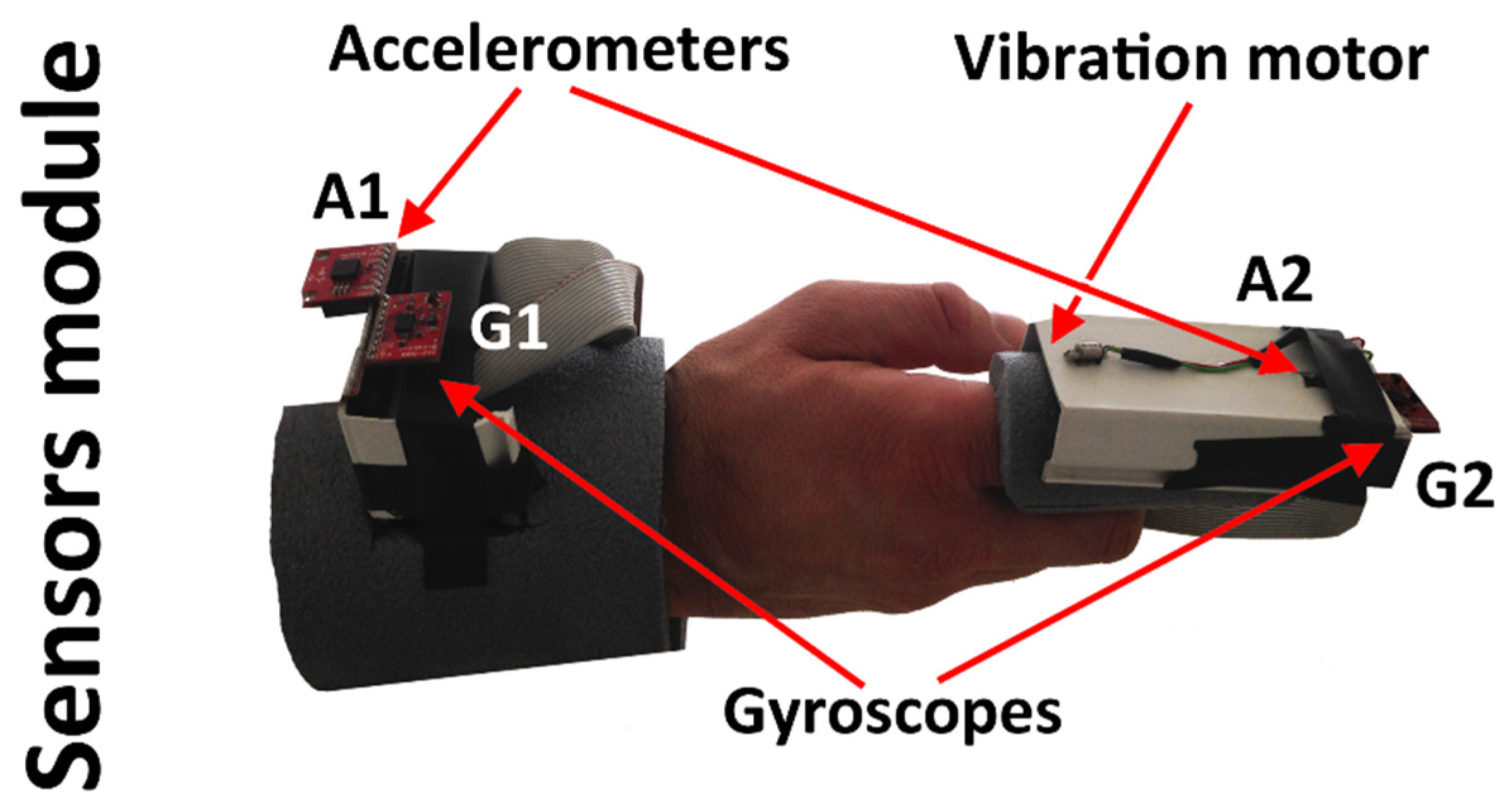
The inertial sensors (accelerometers and gyroscopes) are connected to the wrist and index finger to obtain the data needed to recognize the motion, as shown in Figure 2. Wearable sensors should be small and lightweight, in order to be fastened to the human body without compromising the user’s comfort and allowing her/him to perform the movement under unrestrained conditions as much as possible.
A pattern recognition machine does not perform classification tasks working directly on the raw sensor data. Usually, before the classification, data representations are built in terms of feature variables [28].
The features used in this research are listed in Table 1 [2]. The suggested features are extracted from gyroscopes and accelerometers and are hand-labelled for certain hand motions/gestures. The features selection procedure is described in more detail in [2], where they demonstrated good discriminative power. In essence, raw gyroscope and accelerometer data (and their derivates) from all sensors were plotted in different domains and their correlation to the movement examined, and statistical information was extracted. Based on that, a subset of features was selected, which was then, in turn, further analysed and six of them were finally selected (Table 1). Inclusion of different domains for feature extraction is well-known in inertial-based signals [29].
The first feature is gesture duration, which in some cases cannot be a discriminating feature because it could be the same duration for different gestures. By further analysis, additional features are obtained, such as the second feature that contains local extremes of gyroscope differential data (number of extremes), while the gyroscope axis ratio is the third feature implemented. The fourth and fifth features are derived from accelerometer data and they are the accelerometer axis ratio, which represents absolute acceleration, and movement energy. The last feature is the magnitude of the first significant extreme in the gyroscope data.
Experimental setup and generation of the model for all nine gestures included twenty participants, each of them had ten measurements of all nine performed gestures to generate the reference point for every gesture. Therefore, the proposed model included 1800 labelled hand gestures to form the baseline for the gestures included in process of classification. The participants included healthy subjects of which sixteen were male and four females (aged between 22 and 42). Eighteen subjects were right-handed and two were left-handed. Measurement setup was mounted on right hand of test subjects, and all recording was performed off-line with initial instructions given by an instructor and with opportunity to try performing gestures before actual measurements. Additional details about test subjects and measurement procedure can be found in [2] (database can be found at https://github.com/pinojoke/Gestures_InertialSensors_EAAI (accessed on 31 August 2022)). The hand gestures labelled data are used for the model generation using eight different classifiers, which will be explained in Section 2.2.

2.2. Classification Task

Eight classifiers used in this research are Decision Tree (DT), Random Forests (RF), Logistic Regression (LR), Linear Discriminant Analysis (LDA), Support Vector Machine (SVM) with linear kernel, Naïve Bayes classifier (NB), K-Nearest Neighbours (KNN), and Stochastic Gradient Descent (SGD). The classification task for each of the eight different classifiers is the same and consists of two phases—the training phase and the classification phase. The data were collected during the feature extraction phase and then used to determine the best classifier based on the scoring classifier phase. The scoring phase first divided the dataset into training/validation and testing sets in an 80:20 percent ratio. However, it should be noted that the split was performed on a per-subject basis: one set of subjects was used for training, and completely different subjects were used for testing. This we believe is a more challenging scenario than within-subject testing, and the one enabling more general results and conclusions. Additionally, please note that for hyperparameter optimisation, part of the training set was used to verify the performance, and the test set was used only on the best-performing model configuration.
Next, we trained and optimised the selected classifier and tested the classifier on the test set. For each of the classifiers, the precision, recall, and F-Score have been calculated to show which classifier will achieve the best score. Training of the models, testing, and representation of the results were performed using the combination of MATLAB’s Statistic and Machine Learning Toolbox (https://www.mathworks.com/products/statistics.html (accessed on 31 August 2022)) and Python programming language using the Scikit-learn library (https://www.scikit-learn.org (accessed on 31 August 2022)). Both training and testing were executed on an Intel i5-9400 workstation with 32 GB of RAM and dedicated NVidia GeForce GTX 1080Ti capable of executing ML algorithms. MATLAB was selected as the primary training tool, as it offers a simple and intuitive interface for testing numerous classification learners with options to optimise available hyperparameters for each separate model. As a single 8-bit AVR microcontroller was in charge of data acquisition from several sensors, real-time extraction of features, and controlling the radio transmitter (mobile robot commanded by wireless radio), the selected ML model was required to be as simple as possible, in terms of memory footprint and time required to execute classification task on the microcontroller.

2.2.1. Decision Tree (DT)

The DT is a supervised machine learning approach aimed to solve classification problems by continuously splitting data based on model features [30]. The actual split is performed inside the nodes by questioning the categorical decision variable (the outcome is true or false), while the final decision is in the leaves. The algorithm is commonly represented in a form of a graph, with all choices and results in form of a tree, thus the name of the algorithm.

2.2.2. Random Forests (RF)

The RF classifier algorithm is a notion of the general technique of random decision forests and it is a learning method for classification, regression, and other tasks [31]. RF is a collection of decision trees whose results are aggregated into one final result. The algorithm operates by constructing a multitude of decision trees at training time and outputting the class that is the mode of the classes (classification) or mean prediction (regression) of the individual trees. The ability of RF to limit overfitting without substantially increasing error due to bias is why they are such powerful models. Given a training set X = x 1 , x 2 , ,   x n with corresponding labels Y = y 1 , y 2 , ,   y n , the algorithm selects a random sample with replacement of the training set and fits trees to these samples, and does that repeatedly B times. After training, unseen samples x can be classified by averaging predictions on individual trees (regression), as shown in Equation (1), or by taking the majority vote in decision trees.
f = 1 b b = 1 B f b x

2.2.3. Logistic Regression (LR)

LR is a regression model where the dependent variable is categorical [32]. The binary logistic model is used to estimate the probability of binary response, based on one or more predictor variables (features). LR measures the relationship between the categorical dependent variable and one or more independent variables using a logistic function. LR can be seen as a special case of the generalized linear model and is used in a variety of fields because it is very light and yields good results. Conditional distribution can be Bernoulli or Gaussian because the outcome of the event can be binary (the dependent variable can have only two values). Mathematically, LR is the task of estimating log odds of a certain event, and it estimates multiple linear regression functions as denoted in Equation (2).
l o g r e g p = l o g p y = 1 1 p = 1 = β 0 + β 1 × x i 1 + β 2 × x i 2 + + β p × x i p

2.2.4. Linear Discriminant Analysis (LDA)

LDA, as its name suggests, is a statistical linear model of dimensionality reduction that provides the highest possible discrimination among various classes [33]. It is commonly used in machine learning to find the linear combination of features, which can separate two or more classes of objects with the best performance. While LR is commonly one of the most popular linear classification models that performs well for binary classification but underperforms in cases of multiple classification problems, LDA handles these classes quite efficiently.
The method is based on discriminant functions, which are linear with respect to the characteristic vector, and usually have the form (3):
f t = w t x + b 0
where w represents the weight vector, x the characteristic vector, and b0 a threshold.

2.2.5. Support Vector Machine (SVM) with Linear Kernel

SVM [34] represents a set of related supervised learning methods (supervised learning) that are used for classification and regression. After the initial training SVM model is generated, the classification is performed. The SVM is a binary classifier, i.e., probabilistically classifies data into two categories. The SVM classification is based on a division of all points in space into two categories according to the margin between support vectors, and the algorithm searches for the largest gap between the two categories.
This procedure is referred to as the so-called linear classification; however, to perform the classification of several categories, we perform a kernel trick that implicitly maps the inputs into the multidimensional space. The trick avoids explicit mapping, which is necessary to obtain a linear learning algorithm to be trained with a nonlinear function. Classifier training creates boundary decisions separate from the margin, that must be maximum, and the input dataset so we can obtain a linear distribution of the two classes. Computing the SVM classifier amounts to minimizing an expression of the form is denoted in Equation (4).
1 n   i = 1 n max 0 , 1 y i w x i + b + Λ w 2
The y i are labels for each data sample x i , w is a normal vector that separates the data into two planes, and b is the margin between the hyperplane and classified data. The parameter Λ denotes the trade-off between increasing the margin size and ensuring that x i is inside the right plane.

2.2.6. Naïve Bayes Classifier (NB)

The NB classifier gives a statistical dimension to the made conclusions [35]. Membership in each cluster (class) is determined by the distribution of probabilities. Therefore, optimal classification can be determined by taking into consideration the distribution of probabilities to which each vector belongs (aligning each feature in each group). One of the major advantages of the NB algorithm is the fact that the prediction result is the weighted probability that can then be used later in further computations. Data are presented as n-dimensional vector; the classifier’s task is to predict a group of testing data based on Equation (5).
p V j V a r g m a x ( v j | a 1 ,   a 2 ,   a 3 , ,   a n )
If the Bayesian theorem is applied to Equation (5), Equation (6) is obtained.
V N B = p V j V a r g m a x v j p ( a i | v j )
Set V N B denotes the classified instance and its probability of belonging to a certain class, in this case, one of nine hand gestures.

2.2.7. K-Nearest Neighbours (KNN)

The KNN algorithm is a relatively simple machine learning algorithm that can be used to solve both classification and regression problems [36]. As opposed to LR, LDA, and NB, KNN does not assume any underlying data distribution, but instead, assumes that similar classes exist close in feature space. The algorithm is based on finding the distances between a new input and all the examples in the data. The main advantage of the KNN algorithm is its simplicity for training on small datasets and execution times, but it has a major drawback of slow training with huge training datasets.

2.2.8. Stochastic Gradient Descent (SGD)

SGD [37] is a gradient descent optimisation method for minimizing an objective function (loss function in our case) that is written as a sum of differentiable functions. In both gradient descent and stochastic gradient descent, a set of parameters is updated in an iterative manner to minimize an error function. SGD is one of the fastest training algorithms. SGD is popular for training a wide range of models in machine learning and is a de facto standard for training artificial neural networks. This problem is considered as the problem of minimizing an objective function, as denoted in Equation (7). The parameter w is to be estimated, whilst Q i is associated with observations in the dataset.
Q w = b = 1 B Q i w

2.2.9. Classifiers Evaluation Measures

The comparison of the different classifiers has been performed using the confusion matrices for each of the defined classifiers. The main concepts of confusion matrices are false positive observations (hereinafter denoted as FP), false negatives (FN), true positives (TP), and true negatives (TN). Evaluation measures described in this section are written with binary classification in mind, while multi-class classification, which was used in the paper, was calculated from a confusion matrix by computing metrics for one label versus all other labels as if it had been reduced to a binary problem for each gesture (label) separately. The measurements for the scoring of the particular classifier are defined as follows.
Precision (also called positive predictive value) is a performance measure calculated as the number of correct positive predictions divided by the total number of positive predictions (the sum of false positives and true positives), as shown in Equation (8).
P r e c i s i o n = T P F P + T P
Recall (called sensitivity or true positive rate) measures the proportion of positives that are correctly identified as such. The recall is defined as the ratio of true positive samples and the sum of false negative and true positive samples, as shown in Equation (9).
R e c a l l = T P F N + T P
F1-score is a measure that combines recall and precision in a manner that emphasizes more precision or recall, based on the type of F-score, (10). The measure used in this paper is the F1-score which emphasizes the precision and recall evenly. F1-score is a special case of F with β = 1 and is defined as the harmonic mean of precision and recall, as denoted in Equation (11).
F = 1 + β P r e c i s i o n R e c a l l β 2 P r e c i s i o n + R e c a l l
F 1 = 2 P r e c i s i o n * R e c a l l P r e c i s i o n + R e c a l l

3. Results

The results of the classification are generated by MATLAB with Statistic and Machine Learning Toolbox and Python programming language using Scikit-learn library. Grid search optimisation approach was used to optimise available hyperparameters for each particular model, except SGD (since it demonstrated by far the weakest performance). Parameter search space was different for each machine learning method, depending which parameters were available. Table 2 shows parameters used in optimisation for each method. During optimisation, classification accuracy was used as the goal function. Please note that the table does not contain an exact number of levels for each parameter being tested, but it was considerable for all tested algorithms (as will be shown later on for logistic regression).
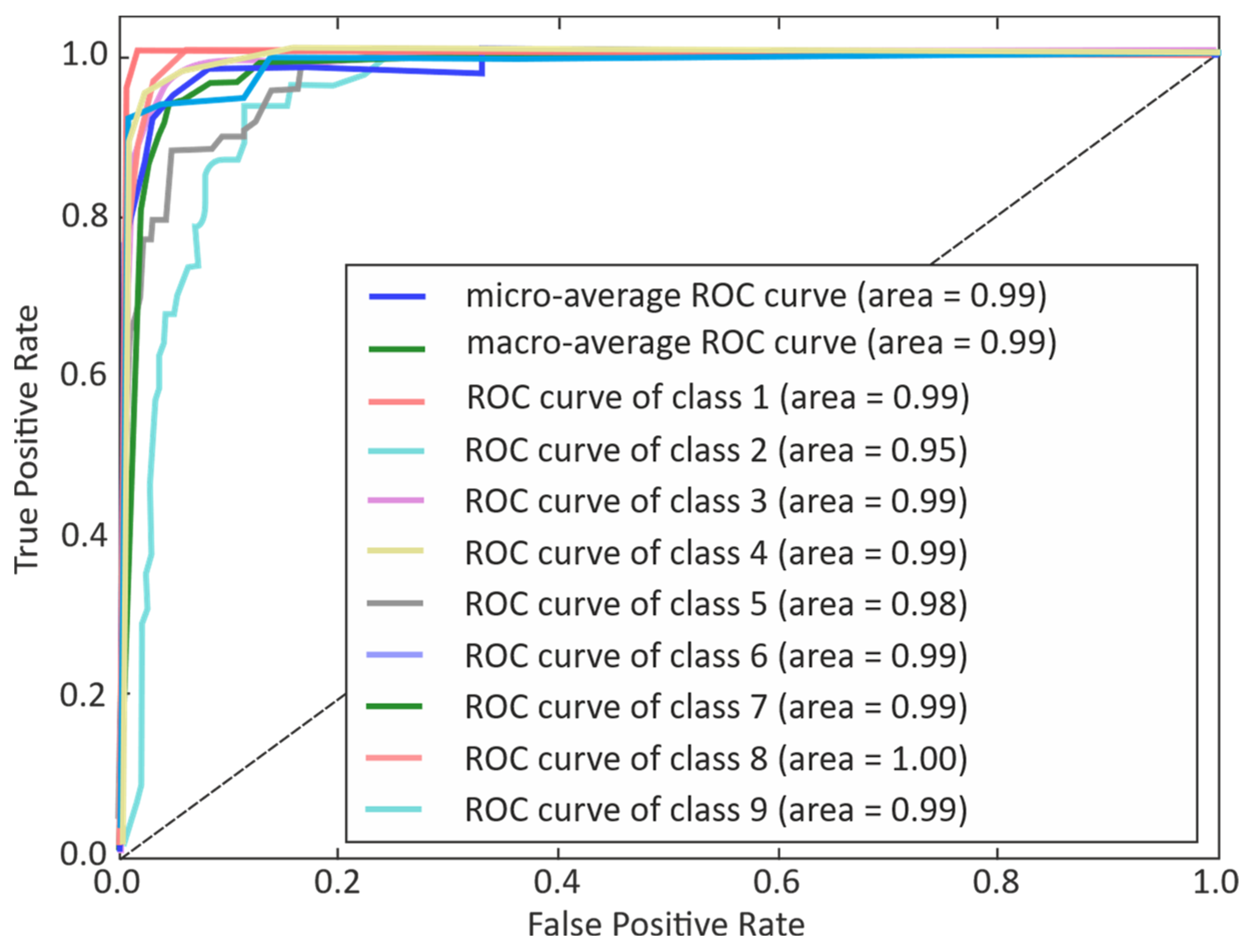
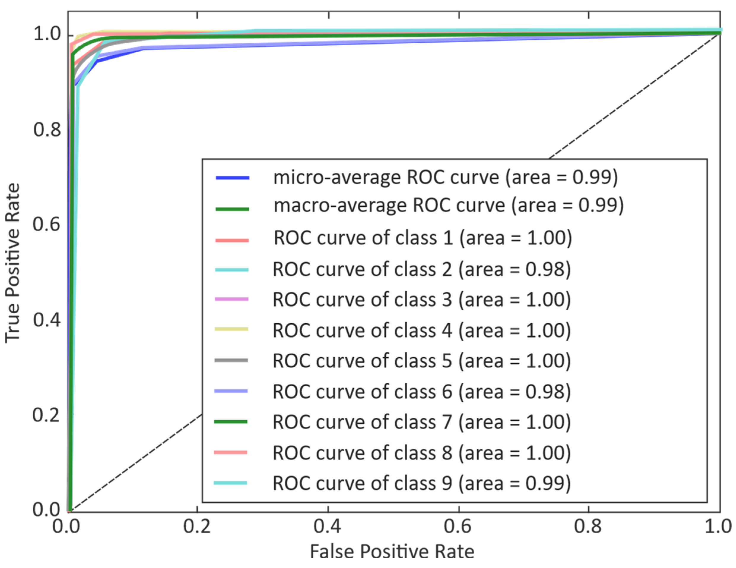
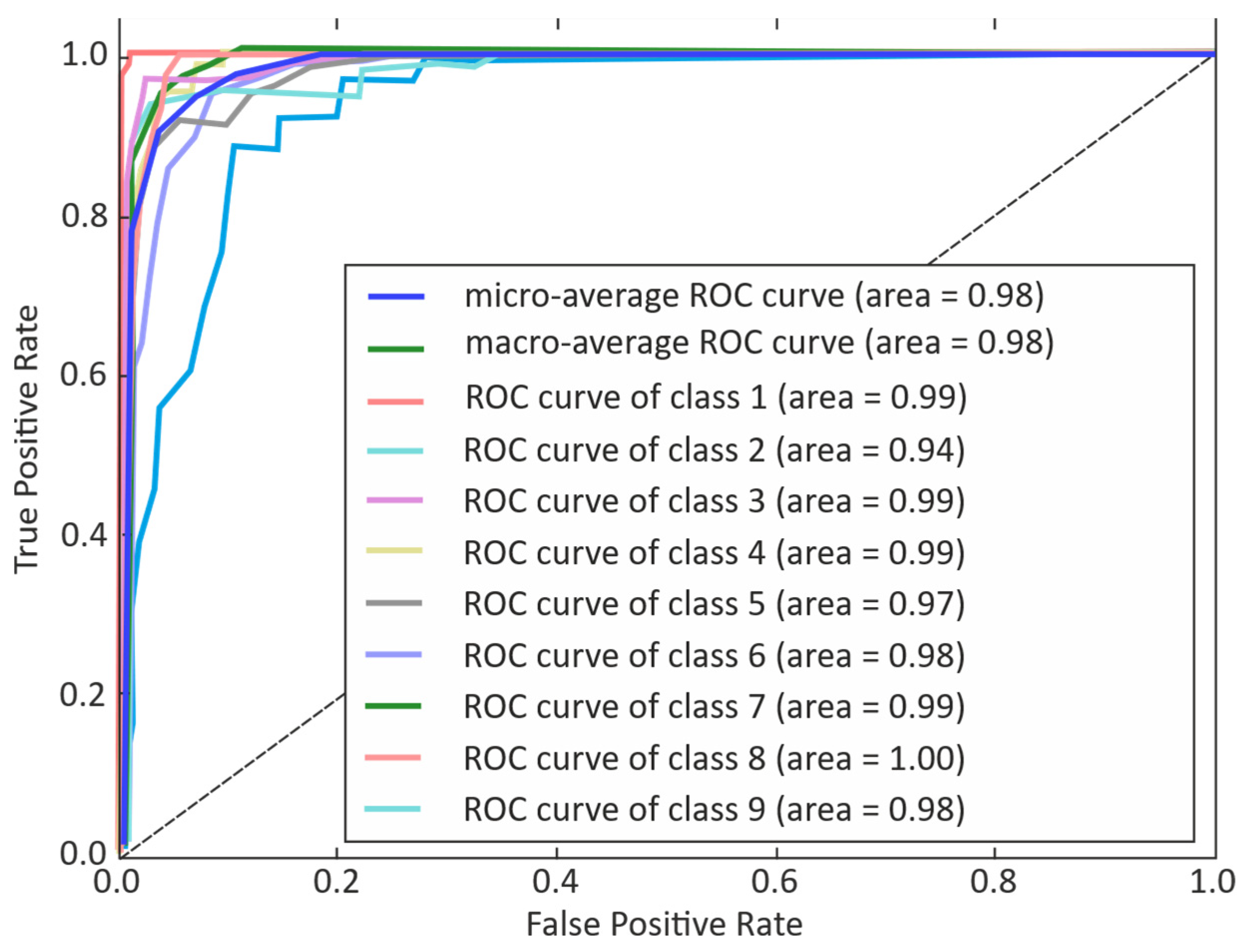
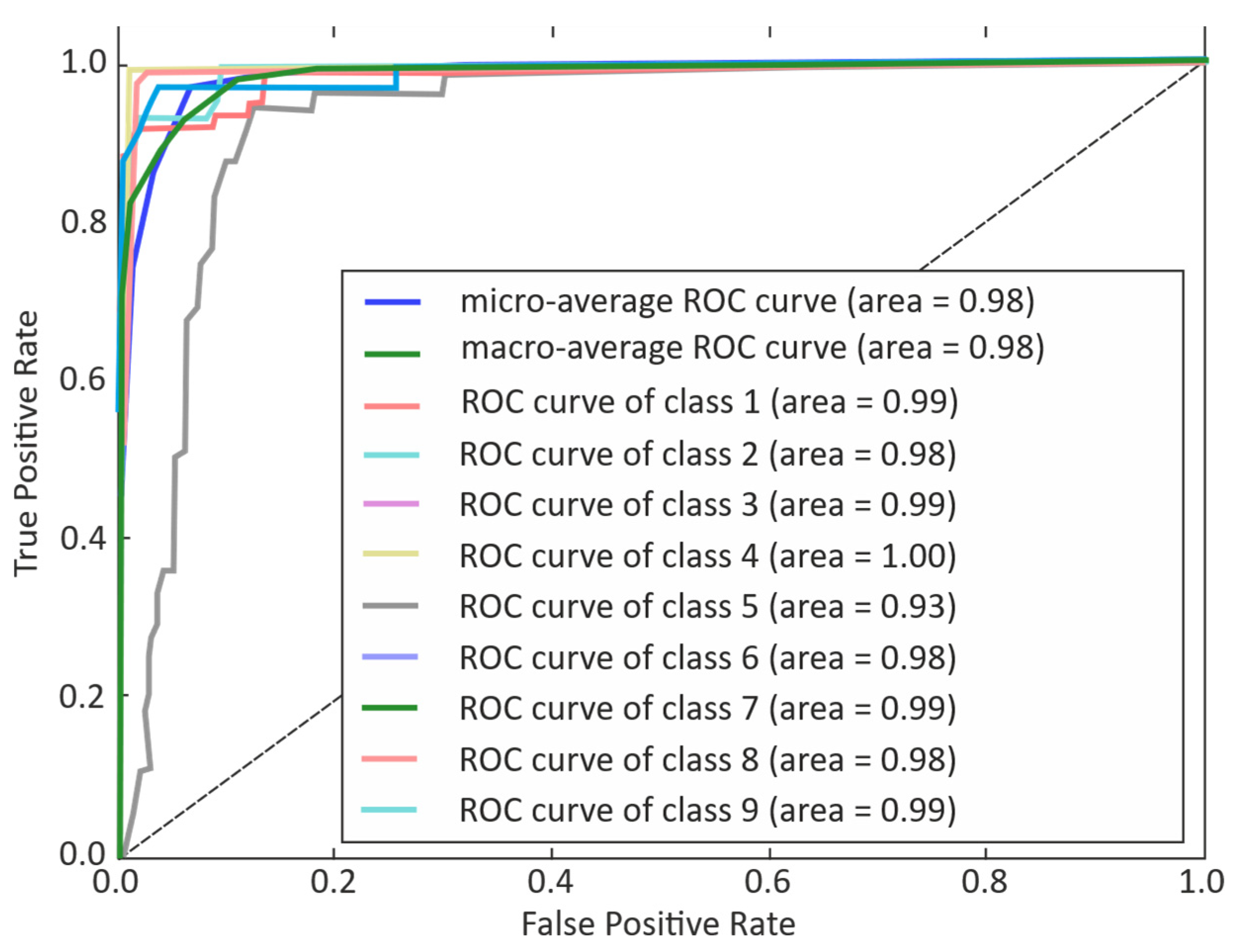
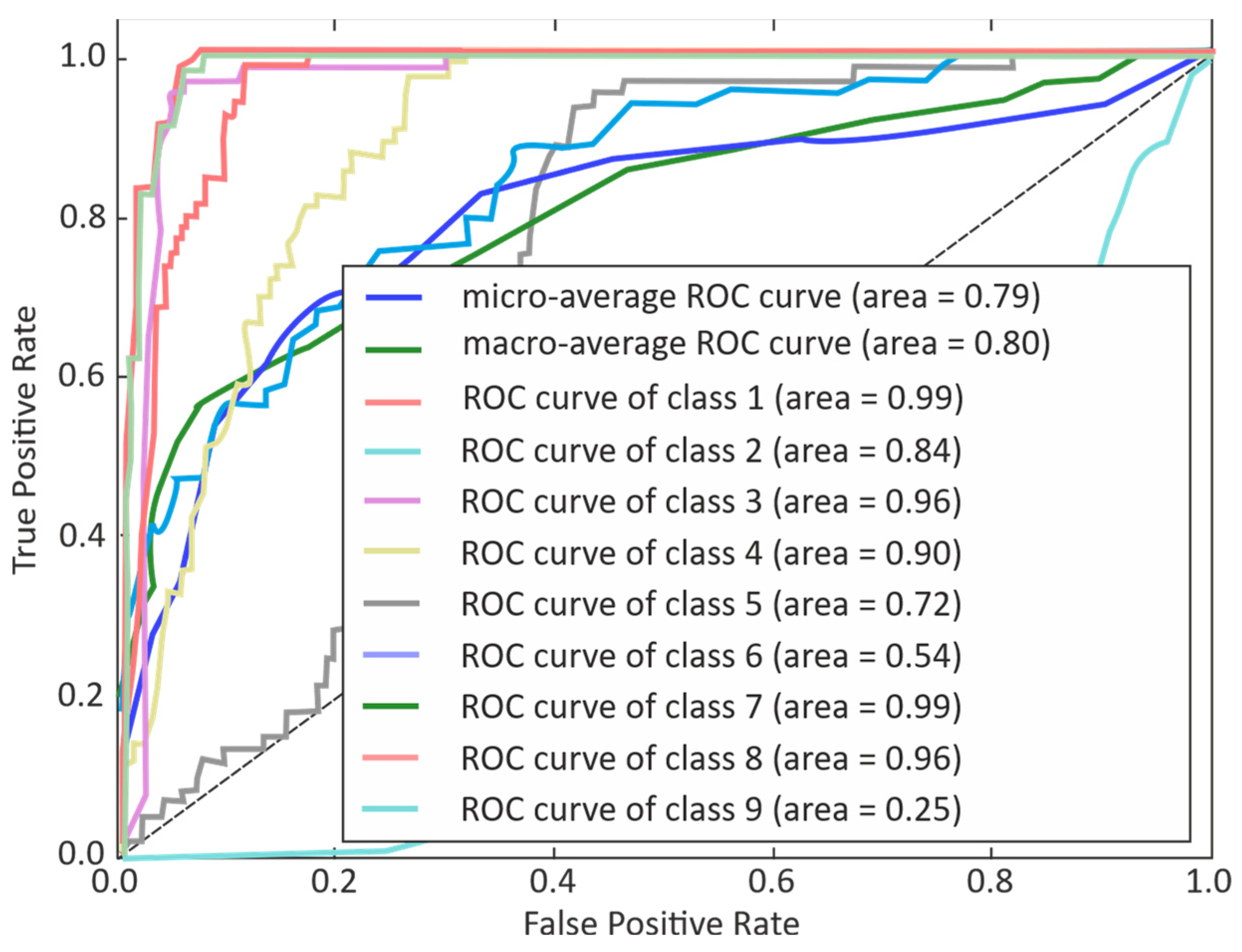
All classifiers were compared, based on precision, recall, and F1-score, as shown in Table 3. When the problem of classification involves the search for the positive class samples, which are very rare compared to the negative classes such as in multi-class classification reduced to a binary problem, by applying the one-versus-all principle, the precision and recall approach is used. This method for the evaluation of classifiers is more useful in “needle-in-haystack”-type problems where the positive class is more “interesting” than the negative class. When it is needed to emphasize negative class, the Receiver Operating Characteristic (ROC) plot is used. ROC curves represent a graphical plot of the True Positive Rate (TPR) as the function of the False Positive Rate (FPR). ROC curves for five selected classifiers are shown in Figure 3, Figure 4, Figure 5, Figure 6 and Figure 7 in order to describe the per-class evaluation results. Other classifiers had similar trends but due to readability issues (they are very similar to the presented ones), were not included. Figures show ROC curves for all nine classes (nine hand gestures) processed with all used classifiers. It is noticeable that the Area under the ROC Curve (AUC) measure as well as the micro-average and macro-average ROC curve are very high (more than 95%) for all classifiers except SGD where the ROC curve is prominently lower. This indicates that SGD classifier underperformed for all classes (gestures) except one and seven.
We also provide Table 4 where the accuracy parameter (as an optimisation goal of hyperparameter grid search) is presented both for the validation set (i.e., the best value obtained during the optimisation, on part of the training dataset) as well as the test set (on the test set with the same hyperparameters as the validation accuracy). Presented values show that there is a difference between performance on the test and training set which was expected. This difference (depending on the machine learning method) varies between 0 and 1.54% (in absolute value) which we believe to be sufficiently small (especially considering that different persons were used in the training and the test set) to conclude that overfitting did not occur. Note that the SGD method is not in the table since optimisation was not performed for it.

4. Discussion

As can be seen from the results in Table 3, the SVM and RF have shown the best results in precision-recall-FI (abbr.: P-R-F1), followed by the KNN and LR. Please note that taking into account the fact that in the test set there were 360 examples, and the difference in obtained results for the three best-performing methods is on the first decimal of the percentage value (0.3% for one, and 0.5% for two misinterpreted gestures), the actual difference comes from the misclassification of only one or two gestures between the approaches. However, when making conclusions about performance it should be kept in mind that a more challenging scenario was used, where training was used on one set of persons and testing was performed on completely different persons (using the same gestures, of course).
According to P-R-F1 measures, the best algorithm is SVM (Kernel function: Gaussian with Box, Optimiser: Bayesian). SVM has certain advantages, such as nice theoretical guarantees regarding overfitting, and with an appropriate kernel, could work well even if data are not linearly separable in the base feature space. Therefore, SVM is especially popular in text classification problems where very high-dimensional spaces are the norm (sparse data). In this case, where the data are clearly linearly separable, SVM with the right parameters can achieve good results, as proven. SVMs are, however, computationally and memory-intensive [20] and thus may require additional optimisation to be effectively executed in resource-limited situations such as, for example, 8-bit AVR microcontrollers.
The second-best algorithm is RF (30 learners and maximum number of splits 1439). It can easily handle feature interactions, and they are non-parametric, so the issue of outliers is not a problem or whether the data are linearly separable. One, and the main, disadvantage is that RF does not support on-line learning, so one must rebuild the tree when new examples are presented. There are also other available variants of ensemble methods (including AdaBoost) that can be used. However, our testing showed that Random Forrest was the best-performing one (in terms of accuracy, i.e., AdaBoost had the best accuracy of 0.978) and was thus chosen as representative for that particular group of methods. However, due to their theoretically faster execution they could be considered as a viable candidate in some instances (but more care should be taken since they are more sensitive to overfitting than the RF).
The third-best algorithm is KNN, (computationally) a simple and easy-to-implement machine learning algorithm and, therefore, potentially suitable for on-line application on 8-bit AVR microcontrollers. The optimal parameters for KNN were: grid search (optimiser), 10 grids (grid division), K = 3 (number of nearest neighbours), and city block as distance metric.
The fourth-best algorithm is the LR classifier, which has a nice probabilistic interpretation, unlike SVM or DT, and one can easily update one’s model to take in new data (using an on-line gradient descent method), again unlike decision trees. Therefore, LR could also be potentially suitable for on-line application on 8-bit AVR microcontrollers, as well as KNN.
The fifth- and sixth-ranked algorithms are LDA and DT, with a slightly poorer performance than SVM, RF, KNN, and LR. For that reason, we do not recommend them for on-line implementation, although, for example, LDA can be trained extremely fast (training time was only 1.3564 s).
One of the simplest classifiers being tested is the NB algorithm, which is also, as LR, probabilistically oriented. The NB classifier will converge quicker than discriminative models, such as LR, so less training data are needed. However, this algorithm is less accurate, as shown in P-R-F1 values and ROC plots.
The last classifier that is tested in this comparison, SGD, is the worst based on used performance parameters. SGD is one of the on-line algorithms that uses a combination of linear functions to solve the minimization problem. Despite the obvious lack of precision, recall, and F1-score in this off-line example, the main advantage of SGD is the light computational cost that is suitable for on-line approaches.
It should be noted that all tested methods were in their vanilla form, without any customizations, and that with certain customization and/or usage of different method variants, different results might be obtained leading to (slightly) different conclusions.
So far, the results suggest that among the four best-ranked classifiers, KNN and LR could be the best solutions for the on-line gesture recognition approach that needs to be implemented on systems requiring low-latency real-time response within resource-restricted environments such as embedded computers and 8-bit microcontrollers. To make the final conclusion of which/whose algorithm(s) could be the most suitable, a more detailed analysis of the application of the best-ranked classifiers on 8-bit microcontrollers is performed, as described in Section 4.1.

4.1. The Applicability of the Best-Performing Algorithms to 8-Bit AVR Microcontrollers

We analysed the applicability of some of the best-performing approaches (based on Table 3 and Table 4) to targeted microcontrollers (8-bit AVR) in terms of a memory footprint as well as computational time (for inference of one, new sample). These results are given in Table 5. From the table, it can be seen that some of the best-performing methods in terms of accuracy and P-R-F1 (SVM and RF) could not be implemented in the targeted device, while some of them (KNN), only in the reduced form (affecting their accuracy). This is marked in Table 5 as KNN—a reduced dataset—meaning that through analysis it was observed that a smaller dataset could be used without sacrificing performance (e.g., accuracy of 0.985 for 460 training samples). Nevertheless, no more than 70 data points were managed to be stored in microcontroller RAM before execution became unstable (and these results are reported in Table 5). However, note that for this small of a dataset, KNN accuracy performance significantly drops, and values in Table 5 for that method are just for illustration purposes.
Only two of the methods (LR and DT) could be implemented, with LR achieving much faster times (18 times) with a somewhat larger footprint (1.8 times). With LR having a better F1-score than DT (0.981 vs. 0.962), this analysis seems to suggest that LR would be the algorithm of choice for targeted application and the device. This also highlights the issue that many similar works often examine only accuracy-related parameters, but do not take into account other, equally important, parameters, such as memory footprint, making viable the need for a standardized applicability measure.
The performed analysis leads to the conclusion that the computational burden (and memory footprint) of the complete classification system can be further reduced. This reduction comes from eliminating the computational time needed to obtain features one and two, as well as using them in the LR model (or any other model), as discussed in Section 4.2. This should in turn make the LR classifier even more appealing for real-time implementation within the embedded systems.
Since LR has proven to be the most computationally appropriate for real-time implementation, we chose to investigate it a bit further.

4.2. More Detailed Discussion Regarding the LR Algorithm

The additional questions we seek to answer were: Could the number of features be reduced to make the model even more appropriate for real-time implementation? If so, what feature could be discarded with no or little effect on the final model performance? Is this applicable to the KNN algorithm?
To answer these questions, we first present, in Table 6, parameter values used in a guided grid search to illustrate the width of our optimal model search. The reason why grid search was guided was the fact that from the literature [38] it is well-established that some solvers and penalties do not mix. For example, while saga solver can handle wall four penalties being tested, the liblinear solver can use only l1 and l2 penalties and lbfgs can use either none or l2.
Taking this into account, alongside dependencies for remaining solvers, this resulted in 8640 combinations being tested in the optimisation procedure. Mean accuracy across all gestures was used as a performance parameter. As a result, eight out of all tested combinations had the same, best performance, and the mean accuracy of 0.981 was obtained. The common denominator for these eight models was the saga solver, while in two cases the l1 penalty was present, and in six others elasticnet. However, elasticnet had faster convergence (100 vs. 500 iterations) and thus was chosen. In all cases, the regularization-related parameter had a value of 0.3 and the parameter ratio a value of 0.5. The difference was only in the tolerance parameter which varied between 0.01, 0.0001, and 0.000001.
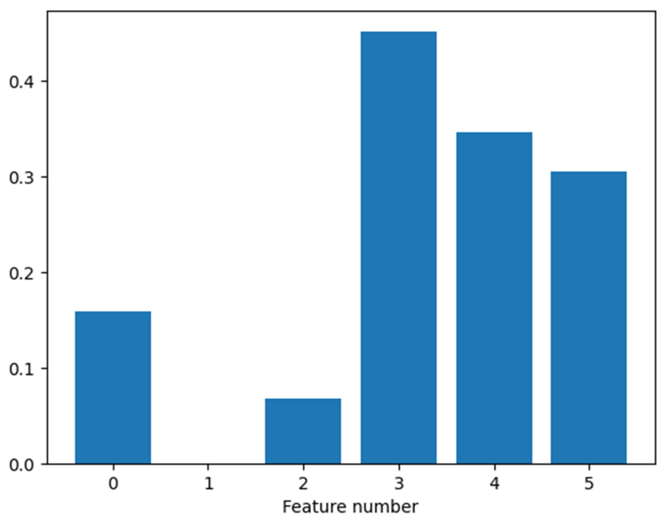
To answer posed questions, the optimised LR model identified previously was chosen as a test base. For feature importance, the permutation approach was used. It is defined as a decrease in a model score (accuracy) when a single feature value was randomly changed [39]. Please note that this type of feature importance is model-independent and it only highlights feature importance in the particular model (and not feature discriminative power by itself). Other approaches to feature importance can also be used, with the same aim of reducing the number of needed features in the considered model while maintaining the desired level of performance. The results of such an analysis are depicted in Figure 8 (the higher the value, the more important the feature is).
From Figure 8, it can be seen that features marked with numbers one and two are the least important, while features three, four, and five seem to be the most important. To verify this fact, the optimal model was run on data without the two lowest ranking features (one and two), and a mean accuracy of 0.969 across all gestures was obtained. This is a decrease of about 1% compared to the full feature model. On the other hand, if the two most important features identified by our analysis (three and four) were omitted from the model, an accuracy of 0.703 was obtained. This is a decrease of about 28%. The same trend (but with different values) was obtained for the KNN classifier: for missing features marked with one and two, the resulting mean accuracy across all gestures was 0.961 (a decrease of about 2%), while for missing features marked with three and four, the resulting mean accuracy across all gestures was 0.878 (a decrease of about 11%). However, please note that if feature importance analysis was performed on the KNN algorithm, different feature importance order might have been obtained due to different model operating principles. This highlights the fact that the permutation-based approach can rank features for a particular model and not in general (i.e., for other models).
It should be noted that a more detailed analysis of other best-performing methods’ optimisation results would also be interesting and could provide some interesting comparative results, but due to a large number of variables considered would significantly increase the length of the analysis. Their implementation in a targeted hardware environment is not feasible, as shown in Section 4.1; thus, in turn, it is omitted.

5. Conclusions

The 8-bit AVR microcontrollers are still widely used in industry and for high-speed signal-processing operations inside embedded systems, such as medical devices used for remote patient monitoring (personal blood pressure monitors, pulsoximeters, and heart rate monitors), and many other applications [27]. However, due to their lack of computational power (i.e., speed) and limited memory available [20], it is a challenging task to efficiently implement different ML algorithms on 8-bit AVR microcontrollers for on-line classification.
The main goal of this research was to test the performance of eight different machine learning algorithms to obtain a robust model which can be efficiently implemented on the 8-bit AVR microcontroller for on-line human gesture recognition and classification with the intention to gesturally control the mobile robot. Having in mind the limited computation power of the 8-bit microcontroller, relatively simple ML algorithms, in terms of memory and processing requirements, were used.
Better data often outperform better algorithms since all tested algorithms depend on the data that are presented as the training set and the design of the high-quality features. The data and features provided in [2] are highly discriminative and, as obtained results show, provide good classification results with the tested ML algorithms. All of the classifiers, except the SGD algorithm, showed very high F1-scores and Area Under Curves (AUCs) in ROC plots.
Regarding the P-R-F1 measures, the two best classifiers proved to be the SVM and RF which showed the highest results (SVM: 0.9865, 0.9861, and 0.9863; RF: 0.9863, 0.9861, and 0.9862). The third-best was KNN (0.9835, 0.9833, and 0.9834), and the fourth-best was LR (0.9810, 0.9810, and 0.9810). The rest of the algorithms (LDA, DT, NB, and SGD) showed slightly poorer performance than SVM, RF, KNN, and LR, and for that reason, were not recommended for the on-line implementation.
Among the best ranking classifiers, SVM and RF are known to be computationally complex; therefore, our assumption was these algorithms would not be suitable for on-line classifications on 8-bit AVR microcontrollers. On the other hand, according to our assumptions stated in the Discussion section, KNN and LR could be potentially suitable for on-line application on 8-bit AVR microcontrollers.
With the aim of confirming the validity of our assumptions, the analysis of the applicability of the best-performing classifiers (based on P-R-F1 measures) to targeted 8-bit AVR microcontrollers in terms of a memory footprint as well as computational time (for inference of one, new sample) was performed.
The analysis confirmed our assumptions regarding the non-applicability of SVM and RF classifiers on 8-bit microcontrollers. Despite our initial assumption regarding the KNN, the analysis proved that KNN is applicable only for reduced datasets since no more than 70 data points were managed to be stored in microcontroller RAM before execution became unstable, while for such a small dataset, KNN accuracy performance significantly decreases. Therefore, the conclusion is that KNN is not suitable for on-line application on 8-bit microcontroller.
However, the analysis for LR proved that this classifier could be efficiently implement on targeted microcontrollers. Having in mind its high F1-score (comparable to SVM, RF, and KNN), this leads us to the conclusion that the LR is the most suitable classifier, among all tested, to be implemented on-line in embedded systems based on 8-bit AVM microcontrollers.
It is also worth noticing that in the paper the extensive fine-tuning of models and hyperparameters optimisation is performed to make them more suitable for the intended task, and suggestions on how to optimise model parameters to achieve the maximum efficiency of the proposed LR algorithm are given.
In future work, to further demonstrate the feasibility of the LR as the proposed algorithm in the on-line scenario, it is planned to implement LR on other mainstream microcontrollers as well and also, to test LR within some available frameworks, such as AIfES (Artificial Intelligence for Embedded Systems) [40], and on other platforms, such as FPGS (Field-Programmable Gate Arrays), with and without the data quantization approach [41].

Author Contributions

Conceptualization, methodology, and formal analysis, I.S., J.M. and M.K.V.; software, M.K.V., I.S. and J.M.; investigation, M.K.V., I.S., J.M. and T.G.; data recording, I.S.; data curation, I.S. and T.G.; validation, all authors; writing—original draft preparation, M.K.V., T.G., J.M. and I.S.; writing—review and editing, all authors; supervision, T.G. and M.B.; project administration and funding acquisition, M.B. All authors have read and agreed to the published version of the manuscript.

Funding

This paper is a result of collaborative research of the scientists participating in two projects, “Computer Vision and Bio-Signal Processing”, and “Computer Intelligence in Recognition and Support of Human Activities”, funded by Faculty of Electrical Engineering, Mechanical Engineering, and Naval Architecture, University of Split, Croatia.

Institutional Review Board Statement

Not applicable.

Informed Consent Statement

Not applicable.

Data Availability Statement

The data presented and analyzed in this study are openly available in: https://github.com/pinojoke/Gestures_InertialSensors_EAAI.

Conflicts of Interest

The authors declare no conflict of interest.

References

  1. Vishwakarma, D.K.; Kapoor, R. An efficient interpretation of hand gestures to control smart interactive television. Int. J. Comput. Vis. Robot. 2017, 7, 454–471. [Google Scholar] [CrossRef]
  2. Stančić, I.; Musić, J.; Grujić, T. Gesture recognition system for real-time mobile robot control based on inertial sensors and motion strings. Eng. Appl. Artif. Intell. 2017, 66, 33–48. [Google Scholar]
  3. Oudah, M.; Al-Naji, A.; Chahl, J. Hand gesture recognition based on computer vision: A review of techniques. J. Imaging 2020, 6, 73. [Google Scholar] [CrossRef] [PubMed]
  4. Molina, J.; Pajuelo, J.A.; Martínez, J.M. Real-time motion-based hand gestures recognition from time-of-flight video. J. Signal Process. Syst. 2017, 86, 17–25. [Google Scholar] [CrossRef]
  5. Chen, Y.-L.; Hwang, W.-J.; Tai, T.-M.; Cheng, P.-S. Sensor-based hand gesture detection and recognition by key intervals. Appl. Sci. 2022, 12, 7410. [Google Scholar] [CrossRef]
  6. Chu, Y.C.; Jhang, Y.J.; Tai, T.M.; Hwang, W.J. Recognition of hand gesture sequences by accelerometers and gyroscopes. Appl. Sci. 2020, 10, 6507. [Google Scholar] [CrossRef]
  7. Tai, T.M.; Jhang, Y.J.; Liao, Z.W.; Teng, K.C.; Hwang, W.J. Sensor-based continuous hand gesture recognition by long short-term memory. IEEE Sens. Lett. 2018, 2, 6000704. [Google Scholar] [CrossRef]
  8. Gupta, H.P.; Chudgar, H.S.; Mukherjee, S.; Dutta, T.; Sharma, K. Continuous hand gestures recognition technique for human–machine interaction using accelerometer and gyroscope sensors. IEEE Sens. J. 2016, 16, 6425–6432. [Google Scholar] [CrossRef]
  9. Lefebvre, G.; Berlemont, S.; Mamalet, F.; Garcia, C. Inertial gesture recognition with BLSTM-RNN. In Artificial Neural Networks; Springer Series in Bio-/Neuroinformatics; Springer: Berlin/Heidelberg, Germany, 2015; Volume 4, pp. 393–410. [Google Scholar]
  10. Jaramillo-Yánez, A.; Benalcázar, M.E.; Mena-Maldonado, E. Real-time hand gesture recognition using surface electromyography and machine learning: A systematic literature review. Sensors 2020, 20, 2467. [Google Scholar] [CrossRef]
  11. Kundid Vasić, M.; Galić, I.; Vasić, D. Human action identification and search in video files. In Proceedings of the 57th International Symposium on Electronics in Marine—ELMAR, Zadar, Croatia, 28–30 September 2015; IEEE: Piscataway, NJ, USA, 2015. [Google Scholar]
  12. Choondal, J.J.; Sharavanabhavan, C. Design and implementation of a natural user interface using hand gesture recognition method. Int. J. Innov. Technol. Explor. Eng. 2013, 10, 249–254. [Google Scholar]
  13. Xu, R.; Zhou, S.; Li, W.J. MEMS Accelerometer based nonspecific-user hand gesture recognition. IEEE Sens. J. 2012, 12, 1166–1173. [Google Scholar] [CrossRef]
  14. Ma, X.; Peng, J. Kinect sensor-based long-distance hand gesture recognition and fingertip detection with depth information. J. Sens. 2018, 2018, 5809769. [Google Scholar] [CrossRef] [Green Version]
  15. Kim, M.S.; Lee, C.H. Hand gesture recognition for Kinect v2 sensor in the near distance where depth data are not provided. Int. J. Softw. Eng. Its Appl. 2016, 10, 407–418. [Google Scholar] [CrossRef]
  16. Karbasi, M.; Bhatti, Z.; Nooralishahi, P.; Shah, A.; Mazloomnezhad, S.M.R. Real-time hands detection in depth image by using distance with Kinect camera. Int. J. Internet Things 2015, 4, 1–6. [Google Scholar]
  17. Li, Y. Hand gesture recognition using Kinect. In Proceedings of the 2012 IEEE International Conference on Computer Science and Automation Engineering, Beijing, China, 22–24 June 2012. [Google Scholar]
  18. Filaretov, V.; Yukhimetsa, D.; Mursalimov, E. The universal onboard information-control system for mobile robots. In Proceedings of the 25th DAAAM International Symposium on Intelligent Manufacturing and Automation, Vienna, Austria, 26–29 November 2014; DAAAM: Vienna, Austria, 2014. [Google Scholar]
  19. Riek, L.; Rabinowitch, T.; Bremner, P.; Pipe, A.; Fraser, M. Cooperative Gestures: Effective signaling for humanoid robots. In Proceedings of the 5th ACM/IEEE International Conference on Human-Robot Interaction, Osaka, Japan, 2–5 March 2010. [Google Scholar]
  20. Ajani, T.S.; Imoize, A.L.; Atayero, A.A. An Overview of Machine Learning within Embedded and Mobile Devices–Optimizations and Applications. Sensors 2021, 21, 4412. [Google Scholar] [CrossRef]
  21. Mazlan, N.; Ramli, N.A.; Awalin, L.; Ismail, M.; Kassim, A.; Menon, A. A smart building energy management using internet of things (IoT) and machine learning. Test. Eng. Manag. 2020, 83, 8083–8090. [Google Scholar]
  22. Cornetta, G.; Touhafi, A. Design and evaluation of a new machine learning framework for IoT and embedded devices. Electronics 2021, 10, 600. [Google Scholar] [CrossRef]
  23. Al-Kofahi, M.M.; Al-Shorman, M.Y.; Al-Kofahi, O.M. Toward energy efficient microcontrollers and Internet-of-Things systems. Comput. Electr. Eng. 2019, 79, 106457. [Google Scholar] [CrossRef]
  24. Dudak, J.; Kebisek, M.; Gaspar, G.; Fabo, P. Implementation of machine learning algorithm in embedded devices. In Proceedings of the 19th International Conference on Mechatronics—Mechatronika (ME), Prague, Czech Republic, 2–4 December 2020; pp. 1–6. [Google Scholar] [CrossRef]
  25. Sakr, F.; Bellotti, F.; Berta, R.; De Gloria, A. Machine learning on mainstream microcontrollers. Sensors 2020, 20, 2638. [Google Scholar] [CrossRef]
  26. Saha, S.S.; Sandha, S.S.; Srivastava, M. Machine Learning for Microcontroller-Class Hardware—A Review. IEEE Sens. J. 2022; accepted. [Google Scholar]
  27. Application Ideas for 8-Bit Low-Pin-Count Microcontrollers. Available online: https://www.digikey.com/en/articles/application-ideas-for-8-bit-low-pin-count-microcontrollers (accessed on 30 August 2022).
  28. Mannini, A.; Sabatini, A.M. Machine learning methods for classifying human physical activity from on-body accelerometers. Sensors 2010, 10, 1154–1175. [Google Scholar] [CrossRef] [PubMed]
  29. Sousa Lima, W.; Souto, E.; El-Khatib, K.; Jalali, R.; Gama, J. Human Activity Recognition Using Inertial Sensors in a Smartphone: An Overview. Sensors 2019, 19, 3213. [Google Scholar] [CrossRef] [PubMed]
  30. Hastie, T.; Tibshirani, R.; Friedman, J. The Elements of Statistical Learning: Data Mining, Inference, and Prediction, 2nd ed.; Springer: Berlin, Germany, 2008. [Google Scholar]
  31. Wai, M.M.N. Classification based automatic information extraction. In Proceedings of the 10th WSEAS International Conference on Communications, Canary Islands, Spain, 24–26 March 2011. [Google Scholar]
  32. McCullagh, P.; Nelder, J. Generalized Linear Models; CRC Press: Boca Raton, FL, USA, 1989. [Google Scholar]
  33. Izenman, A.J. Linear discriminant analysis. In Modern Multivariate Statistical Techniques; Springer Texts in Statistics; Springer: New York, NY, USA, 2013. [Google Scholar] [CrossRef]
  34. Cortes, C.; Vapnik, V. Support-vector networks. Mach. Learn. 1995, 3, 273–297. [Google Scholar] [CrossRef]
  35. Pardos, Z.; Heffernan, N. Modeling individualization in a Bayesian networks implementation of knowledge tracing. In Proceedings of the International Conference UMAP, Big Island, HI, USA, 20–24 June 2010. [Google Scholar]
  36. Burkov, A. The Hundred-Page Machine Learning Book; Burkov, A., Ed.; Andriy Burkov: Quebec City, QC, Canada, 2019. [Google Scholar]
  37. Chen, J.; Melo, G.D. Semantic information extraction for improved word embeddings. In Proceedings of the NAACL-HLT, Denver, CO, USA, 31 May–5 June 2015. [Google Scholar]
  38. Scikit-Learn: Machine Learning in Python. Available online: https://scikit-learn.org/stable/modules/generated/sklearn.linear_model.LogisticRegression.html#sklearn.linear_model.LogisticRegression (accessed on 1 July 2022).
  39. Breiman, L. Random forests. Mach. Learn. 2001, 45, 5–32. [Google Scholar] [CrossRef]
  40. AIfES for Arduino. Available online: https://github.com/Fraunhofer-IMS/AIfES_for_Arduino (accessed on 20 July 2022).
  41. Coelho, C.N.; Kuusela, A.; Li, S.; Zhuang, H.; Ngadiuba, J.; Aarrestad, T.K.; Loncar, V.; Pierini, M.; Pol, A.A.; Summers, S. Automatic heterogeneous quantization of deep neural networks for low-latency inference on the edge for particle detectors. Nat. Mach. Intell. 2021, 3, 675–686. [Google Scholar] [CrossRef]
Figure 1. Time sequence of nine gestures used in experiments for hand gestures recording and identification. Reprinted from [2], Copyright 2017, with permission from Elsevier.
Computation 10 00159 g001
Figure 2. Sensors module with marked sensor locations. Reprinted from [2], Copyright 2017, with permission from Elsevier.
Computation 10 00159 g002
Figure 3. ROC plot for SVM classifier (micro-averaged 99%).
Computation 10 00159 g003
Figure 4. ROC plot for RF classifier (micro-averaged 98%).
Computation 10 00159 g004
Figure 5. ROC plot for LR classifier (micro-averaged 99%).
Computation 10 00159 g005
Figure 6. ROC plot for Gaussian NB classifier (micro-averaged 98%).
Computation 10 00159 g006
Figure 7. ROC plot for SGD classifier (micro-averaged 79%).
Computation 10 00159 g007
Figure 8. Permutation features important values for optimised LR model.
Computation 10 00159 g008
Table 1. Features for off-line evaluation with selected classifiers. Adapted from [2], Copyright 2017, with permission from Elsevier.
Feature NameFeature DescriptionSensors Used 1
Gesture durationGesture duration in msG1, G2
Number of extremesNumber of extremes from differential gyroscope data (DGD)G1, G2
Gyroscope axis ratioMean ratio of axis of DGD, detects direction of motionG1, G2
Accelerometer ratioMean ratio A1 axis, detects hand orientationA1
Movement energyIntegrates absolute A1 and A2 magnitude over the duration of the whole gestureA1, A2
First rotation direction (flexion or extension)Magnitude of the first large DGD peak, detects hand rotation directionG1, G2
1 As in Figure 2: G1 is the wrist gyroscope, G2 is the index finger gyroscope, A1 is the wrist accelerometer, A2 is the index finger accelerometer.
Table 2. Optimised parameters for each particular model (except SGD).
ClassifierOptimised Parameter
Decision tree (DT)Maximum number of splits
Random Forests (RF)Maximum number of splits, Number of learners, Ensemble method
Logistic Regression (LR)Solver, Penalty, Regularization strength, Convergence tolerance and maximum number of iteration steps, Elastic-Net mixing parameter
Linear Discriminant Analysis (LDA)Discriminant type, solver
SVMKernel function, Optimiser
Naïve Bayes (Gaussian) (NB)Iterations, Acquisition function, Optimiser
The K-Nearest Neighbours (KNN)Optimiser, Number of grid divisions, Distance metric, Number of nearest neighbours
Stochastic Gradient Descent (SGD)#none
Table 3. Precision, Recall, and F1-score Measures for Classifiers Comparison, in descent order regarding P-R-F1 measures.
PrecisionRecallF1-Score
SVM0.98650.98610.9863
Random Forests (RF)0.98630.98610.9862
K-Nearest Neighbours (KNN)0.98350.98330.9834
Logistic Regression (LR)0.98100.98100.9810
Linear Discriminant Analysis (LDA)0.96530.96100.9631
Decision tree (DT)0.96170.96210.9620
Naïve Bayes (Gaussian) (NB)0.94320.91780.9303
Stochastic Gradient Descent (SGD)0.28800.41200.2900
Table 4. Accuracy of different machine learning algorithms on test (validation) set and test set for best-performing parameter configuration.
Validation AccuracyTest Accuracy
Random Forests (RF)0.98610.9861
Linear SVM0.98400.9861
K-Nearest Neighbours (KNN)0.97800.9832
Logistic Regression (LR)0.98050.9651
Decision tree (DT)0.95400.9616
Linear Discriminant Analysis (LDA)0.92400.9609
Naïve Bayes (Gaussian) (NB)0.90700.9185
Table 5. Implementation results for memory footprint and inference time on 8-bit AVR microcontroller.
ML MethodFLASH (kB)RAM (kB)Inference Time (ms)
SVM70.2638.54N/A *
Random forest (RF)163.95187.3N/A *
KNN (reduced dataset)26.190.581.5
Logistic regression (LR)2.970.200.04
Decision Tree (DT)1.630.240.716
* N/A indicates that the appropriate methods could not be reliably implemented in the microcontroller using standardized model and libraries.
Table 6. LR parameters and their values used for grid search optimisation.
ParameterValue
Solvernewton-cg, lbfgs, liblinear, sag, saga
Penaltynone, l1, l2, elasticnet
Inverse of regularization strength (C)10−7, 10−6, 10−5, 3 × 10⁻⁵, 10−4, 3 × 10⁻⁴, 10−3, 3 × 10⁻³,
10−2, 3 × 10⁻², 10−1, 2 × 10⁻¹, 25 × 10−2, 3 × 10⁻¹,
35 × 10−3, 6 × 10⁻¹, 8×10⁻¹, 1, 2, 5
Tolerance for stopping criteria10−6, 10−5, 5 × 10⁻², 10−3, 5 × 10⁻¹, 10−2, 10−1, 1, 2
Maximum number of iterations for convergence50, 100, 500
Elastic-Net mixing parameter (rati) 10.2, 0.4, 0.5, 0.6, 0.8
1 Only used when elasticnet penalty was considered.
Publisher’s Note: MDPI stays neutral with regard to jurisdictional claims in published maps and institutional affiliations.