1. Introduction
The range of areas in which autonomous mobile systems are used is growing continuously. The use of autonomous transport vehicles in industry or robots in private households has now become standard. The development of autonomous motor vehicles is also progressing steadily. Machine learning offers the field of robotics a set of tools for designing difficult and complex behaviors. Furthermore, the challenges of robotics-related problems also provide a positive impact on developments in robot learning.
In all use cases, the basic challenge is the same. Autonomous mobile systems must simultaneously estimate their position in an unknown environment and simultaneously create a map of the environment. This challenge is also referred to as the SLAM problem. While filter-based approaches such as [
1] were the most common solution for this problem before 2010; graph SLAM and its derivatives are now the most popular and efficient approach [
2,
3]. In this approach, a robot’s landmarks and poses are represented by a graph, which allows the SLAM problem to be solved via nonlinear optimization techniques [
4,
5].
The SLAM problem refers to the difficulty of locating and mapping a mobile robot in an unknown environment with its simultaneous positioning relative to this map [
1]. When no other navigation capabilities, such as the Global Navigation Satellite System (GNSS), are available, the SLAM problem becomes more important [
6,
7]. While already solving the problem in simple applications, SLAM algorithms can be pushed to their limits by challenging dynamic robot motions or highly dynamic environments [
4,
8]. To obtain a map, sensors must be used to detect the structure of the environment. A variety of possible sensor types are available for this purpose.
Finally, by determining the position of the environmental features, it is possible to obtain a representation of the robot’s environment and thus a map that can be used in numerous ways, such as localization. The basic problem within SLAM is to estimate the trajectory of the robot as well as the position of all environmental features without knowing the true position of the features or the robot itself [
1,
9]. Since their advent and rapid improvement in cost and efficiency in recent years, LiDAR sensors play a key role in sensing the environment of mobile systems [
10,
11]. The incorporation of dense 3D point clouds in existing localization systems posed significant problems concerning the achievable precision of the point cloud matching and the update rate of other employed systems such as inertial measurement units (IMU), global navigation satellite systems (GNSS), and optical systems. Modern SLAM systems such as HDL-Graph-SLAM [
12] employ a graph-based and efficient approach for sensor fusion by solving the SLAM problem.
Alas, it remains a difficult task to assess the hyperparameters of these algorithms, such as choosing the right scan matching algorithm and the overall accuracy [
13]. The common lack of precise external systems is overcome in this article by using a low-cost real-time kinematics GNSS system (RTK-GPS), which allows for precise localization of the mobile system up to a precision of 2 cm. As the system shall be applicable to many institutions and smaller companies, we provide an evaluation of the accuracy of both, the underlying 3D-SLAM system and the chosen evaluation system, by comparing different scenarios and testing situations. This makes it possible to identify the correct settings, sensors, and application cases for the systems in soft- and hardware.
This article is organized as follows.
Section 2 describes the materials and methods used.
Section 3 contains a discussion of the experimental results.
Section 4 concludes the paper.
2. Materials and Methods
Since the DARPA’s Urban challenge in 2008, 3D laser scanners are typically used for autonomous driving. They are built up of several lenses and beams, which are usually arranged in groups of 16, 64, or 128 in a vertical fan pattern. This allows the capturing of multiple planes and distances to be scanned simultaneously [
14,
15].
GNSS systems play a crucial role in localization and navigation for mobile systems. The advent of RTK-GNSS (Real Time Kinematic positioning) systems allows for the localization up to a precision of centimeter level. Still, the systems suffer from broken line-of-sight toward the base station as well as the shadowing from buildings, signal loss within closed buildings or tunnels, and problems under dense vegetation.
To assess the capability of our mobile robot in combination with the proposed sensor suite of LiDAR, IMU, and odometry, the RTK-GNSS solution is intended to work as a ground truth system to give a measure of quality for the overall setup.
2.1. Main Hardware Components
2.1.1. LiDAR System
The OS1 LiDAR from Ouster was used in this work.
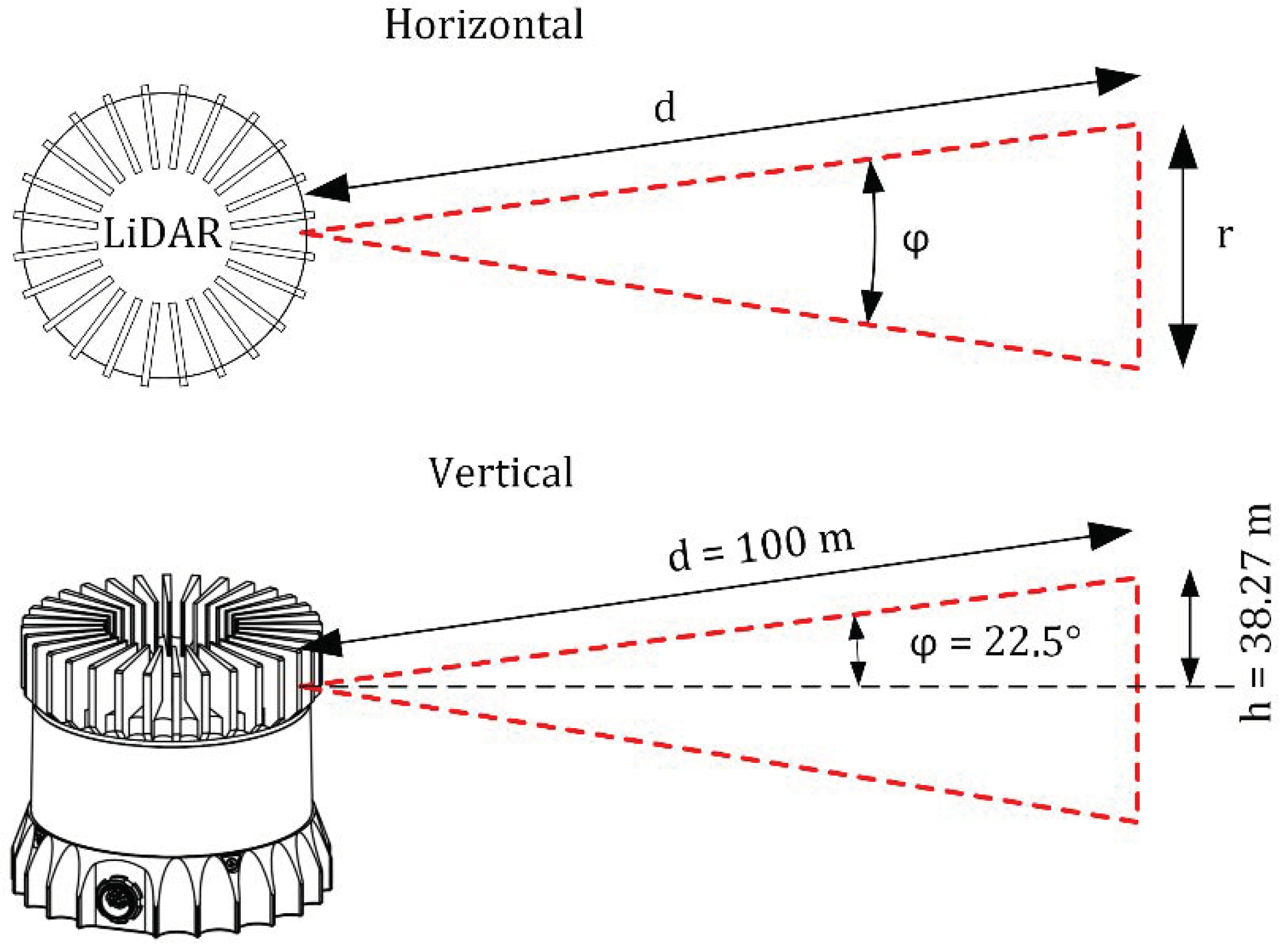
It is suitable for distances between 0.3 and 100 m and has a vertical field of view of 45° (±22.5°). It has a vertical resolution of 128 lines and a configurable horizontal resolution of 512, 1024, or 2048 lines. Depending on the resolution, the LiDAR sensor can scan its environment at 10 or 20 Hz. Thus, at a resolution of 128 × 2048 and the frequency of 10 Hz, up to 2,621,440 points can be captured by the sensor within one second, corresponding to a data rate of up to 254 Mb/s [
16].
For later outdoor applications, the raster size is also of interest. The determination of raster size with which the environment is scanned, as a function of the distance, can be determined using trigonometric relationships. This relationship is shown in
Figure 1.
The maximum distance of 100 m is considered, which is particularly interesting for outdoor applications. Furthermore, a distance of 10 m is considered for the indoor area. The raster values, depending on the resolution and the distance, are listed in
Table 1.
2.1.2. Real Time Kinematics GNSS
RTK systems are based on the working principle of differential GPSd by a so-called rover to precisely estimate its position [
18]. In contrast to common DGPS, the positioning is based on the carrier measurement, not the pseudo-code signals. RTK systems for surveying or precise civil engineering measurement are well established but are also expensive [
19].
GNSS signals provide useful position information in the range of meters, which can easily be incorporated and used to enhance the position estimate in a broad range of sensor fusion architectures [
1,
6].
To verify the accuracy of the SLAM localization and trajectory estimation, we used the C94-M8P, a low-cost RTK-GPS system from ublox. Besides the experimental evaluation and assessment of the LiDAR-SLAM accuracy, the low-cost nature allows for a possible integration within the system as an additional sensor to enhance localization accuracy in unobstructed environments and to fasten up initial localization within a map.
2.1.3. Husky A200
The unmanned ground vehicle (UGV) “Husky A200” from Clearpath Robotics is used for this work. The robot platform, which is equipped with an all-wheel drive, can be remotely controlled with the aid of a controller.
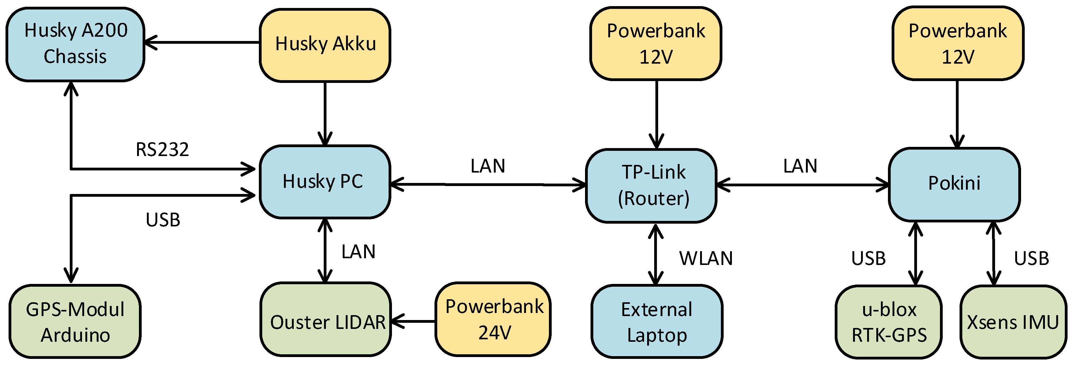
A structural diagram of the hardware setup is shown in
Figure 2. Inside the Husky is the main computer, which contains the basic system for the Husky. When the rover is switched on, the main computer and thus all necessary processes are started automatically [
20].
ROS Structure Husky
When the Husky is started, a ROS core, which represents the master, is automatically started on the Husky computer. All necessary ROS packages that are required for the operation of the Husky are executed. The hardware setup, as described in
Figure 2 allows for subscribing or publishing the desired topics from any computer, enabling easy cross-network data exchange.
2.2. Main Software Components
2.2.1. Robot Operating System
ROS (Robot Operating System) is an open-source platform for programming robot systems. It is a meta-operating system that provides various tools for simulation and visualization as well as libraries. The libraries mainly include hardware abstractions as well as device drivers for sensors and actuators [
21].
ROS is a peer-to-peer network, which means that all participants have equal rights and that services can be offered and used. The individual participants can be distributed over several computers, whereby they are loosely coupled by the ROS communication infrastructure. To organize communication, there is exactly one master in each ROS network that manages communication and with which each node must be registered [
22,
23].
2.2.2. Scan Matching Algorithms
With each scan of a LiDAR sensor, a point cloud with measurement points is obtained, as shown in the previous section. To use these point clouds for mapping or localization in a map, the challenge is to match the current scan with an already known scan of the surrounding area. The process of matching two scans is also called registration. Two main algorithms emerged as viable options for 3D-point-cloud registration, the classical iterative closest point (ICP) algorithm [
24] and a more refined version, the generalized ICP. In addition, the normal distributions transform (NDT) of [
25] is considered, as it takes a different approach based on data statistics.
Iterative Closest Point (ICP)
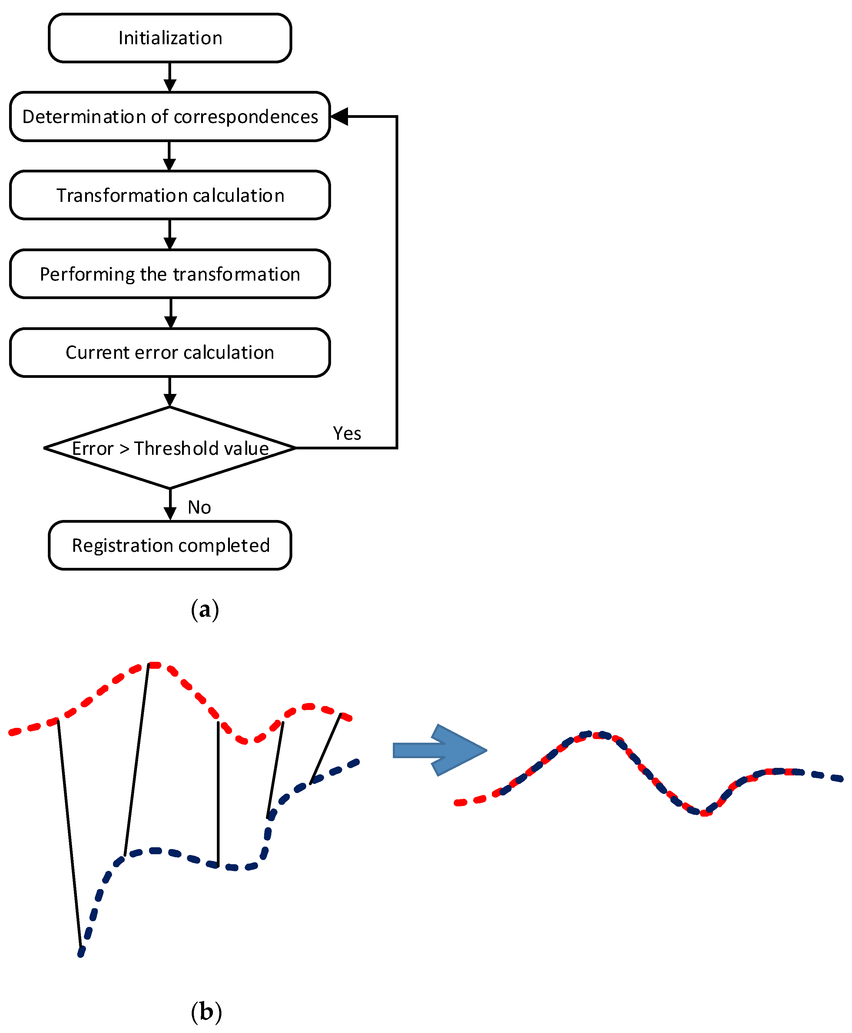
Iterative closest point (ICP) is an algorithm used in many applications to achieve a minimum difference between two-point clouds. The flowchart of the ICP algorithm is illustrated in
Figure 3a, and its basic idea is illustrated in
Figure 3b.
To be able to calculate the rotation and translation, the point correspondences must first be determined, i.e., which point of the blue point data set to be transformed corresponds to which orange point of the base point data set. As the simplest measure for the determination of the point correspondences, the Euclidean distance is used. Thus, the correspondences match the points with the smallest distance. Once the point correspondences have been determined, the calculation and execution of the transformation are performed for each point. Then, the current error between the transformed points (blue) and the base point data set (red) is determined. If the error is above a previously defined threshold, a new iteration is started, and the point correspondences are determined again. If the error is below the specified threshold or the maximum number of iterations is reached, the registration of the two scans is completed [
26].
Voxelized Generalized Iterative Closest Point Algorithm (VGICP)
To overcome the problems of ICP and NDT, the examined HDL Graph SLAM algorithm uses another registration method, the VGICP algorithm. This approach can be seen as a combination of the ideas of the aforementioned methods, as it extends the generalized ICP approach by determining the distribution of points in voxels, similar to the NDT method, which is achieved by aggregating the individual point distributions within the voxels. In the GICP method, all points are modeled by distribution, and the point correspondence is determined by the smallest distance between two distributions. The procedure is precise but also computationally intensive. In the NDT method, registration is accelerated by using a point-to-voxel distribution correspondence model. However, to compute a 3D covariance matrix, at least ten points within a voxel are needed in practice. If the number of points within the covariance matrix is too small, the covariance matrix will be distorted. In the VGICP method, the covariance matrix is determined from the individual point distributions. This results in a correct covariance matrix even if there is only one point within the voxel. Correspondence determination in VGICP is then performed using a “single-to-multiple-distribution” model according to [
14].
SLAM
The SLAM problem (simultaneous localization and mapping) deals with the problem of simultaneously estimating the position of a robot or sensor in an unknown environment while gradually creating a map of the environment. Sensors used here are usually wheel encoders, IMU, LiDARs, or cameras. There are three main paradigms used to solve the SLAM problem, from which further approaches are derived.
Classical systems use the Extended Kalman Filter for data fusion and landmark-based localization (see [
1]). Multiple locations and the need to deal with lost and kidnapped robots lead to particle filter-based SLAM methods, with FastSLAM as the most prominent [
27].
More recent approaches are either based on a rearrangement of the probabilistic graph of the underlying Bayes Filter (see [
28,
29] for further details) to solve the probability integral more efficiently or they embrace the Graph-SLAM paradigm, in which the SLAM problem is solved in the least squares sense via non-linear iterative optimization techniques [
5,
6]. These methods find widespread applications in camera-based systems, commonly called visual SLAM [
30,
31] or scan matching based applications for 2D laser scan systems.
Due to the wide availability and further development of nonlinear optimization, Graph-SLAM has been the most popular and efficient approach for autonomous mobile systems since 2010 [
32,
33].
LiDAR sensors provide 3D scans of the environment at a frequency of typically 10 Hz, resulting in a large volume of data. The changes between individual scans are often minimal with only a small change in translation and rotation of the robot. To reduce the complexity and the amount of data, only selected scans, so-called keyframes, are often used to create a pose graph, which is used to locally anchor new scans. Thus, a new node is added to the graph only when the pose of the robot has significantly changed translationally and rotationally. Most important for the improvement of scan systems and algorithms has been the advent of inexpensive 3D LiDAR scanners such as the one used in this contribution.
HDL Graph SLAM
HDL Graph SLAM is a real-time SLAM algorithm for 3D laser scanners. It is based on a 3D graph SLAM with an NDT-like scan matching procedure to determine the trajectory. HDL Graph SLAM is suitable for six degrees of freedom. In addition to scan matching, other sensor inputs such as IMU or GPS can be used as boundary conditions (edges) for trajectory determination.
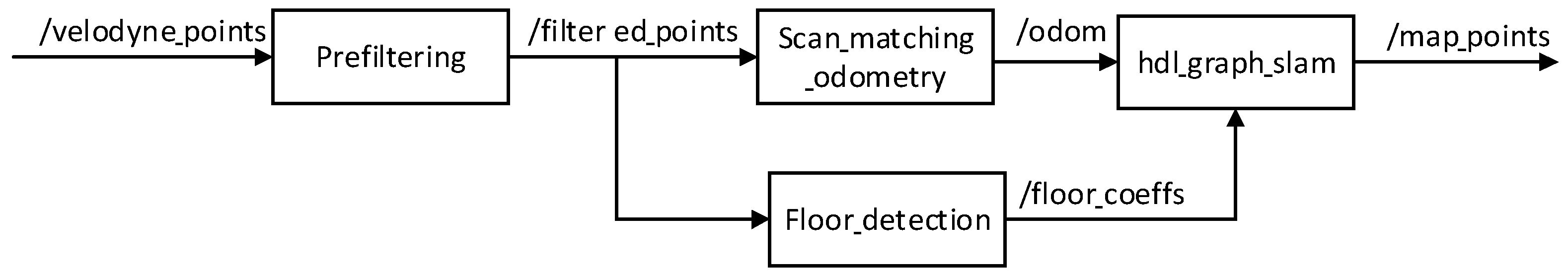
Figure 4 shows an overview of the four nodes that make up the hdl_graph_slam [
34]. After preprocessing the input point clouds, the filtered point clouds are processed by the scan_machting_odometry node for trajectory estimation and in a second step for ground surface detection. Using the outputs of both nodes, the trajectory is afterward optimized in the hdl_graph_slam node, resulting in the desired output map, which consists of registered 3D points.
Prefiltering Node
In the prefiltering node, the laser scan data are preprocessed. The measurement points that are too close or too far away are removed. This can be defined via the threshold values distance_near_thresh and distance_far_thresh.
Furthermore, the outliers can be removed from the point clouds in the prefiltering step. For this purpose, a radius method or a statistical method can be applied. The radius method considers the number of neighbors of a point that lie within the given radius (radius_radius). If the value is below the minimum number of neighbors (radius_min_neighbours), the point is removed. In the statistical method, outliers can be determined and removed via the standard deviation (statistical_stddev).
Scan_matching_odometry Node
Scan matching is performed using the filtered points. The sensor pose is estimated by applying a scan matching method from successive frames, from which the trajectory of the robot is determined (odometry estimation). For scan matching, the methods ICP, GICP, NDT, and VGICP described in
Section 2.2.2 can be selected, and the corresponding parameters for the algorithms can be configured.
Floor_detection Node
In buildings with larger indoor areas, such as schools or hospitals, the surrounding area often has only one flat floor surface. To optimize the pose graph, an additional boundary condition was therefore introduced that takes into account the detected floor area. For this purpose, it is assumed that all floor surfaces detected in the respective scan lie on the same plane. For configuration, the estimated sensor height (
sensor_height) must be specified. To estimate the ground plane, all points that are within a given range above or below the ground height (
hight_clip_range) are used. The estimation of a plane is performed using RANSAC (random sample consensus). RANSAC is a robust algorithm for estimating a model, e.g., a plane, within a point cloud containing outliers. For an estimated plane to be accepted, there must be a minimum number of points (
floor_points_thresh) within the
hight_clip_range, the estimated plane. If there are fewer points or if the plane is tilted by more than a 10° angle (
floor_normal_thresh), the plane is not accepted. [
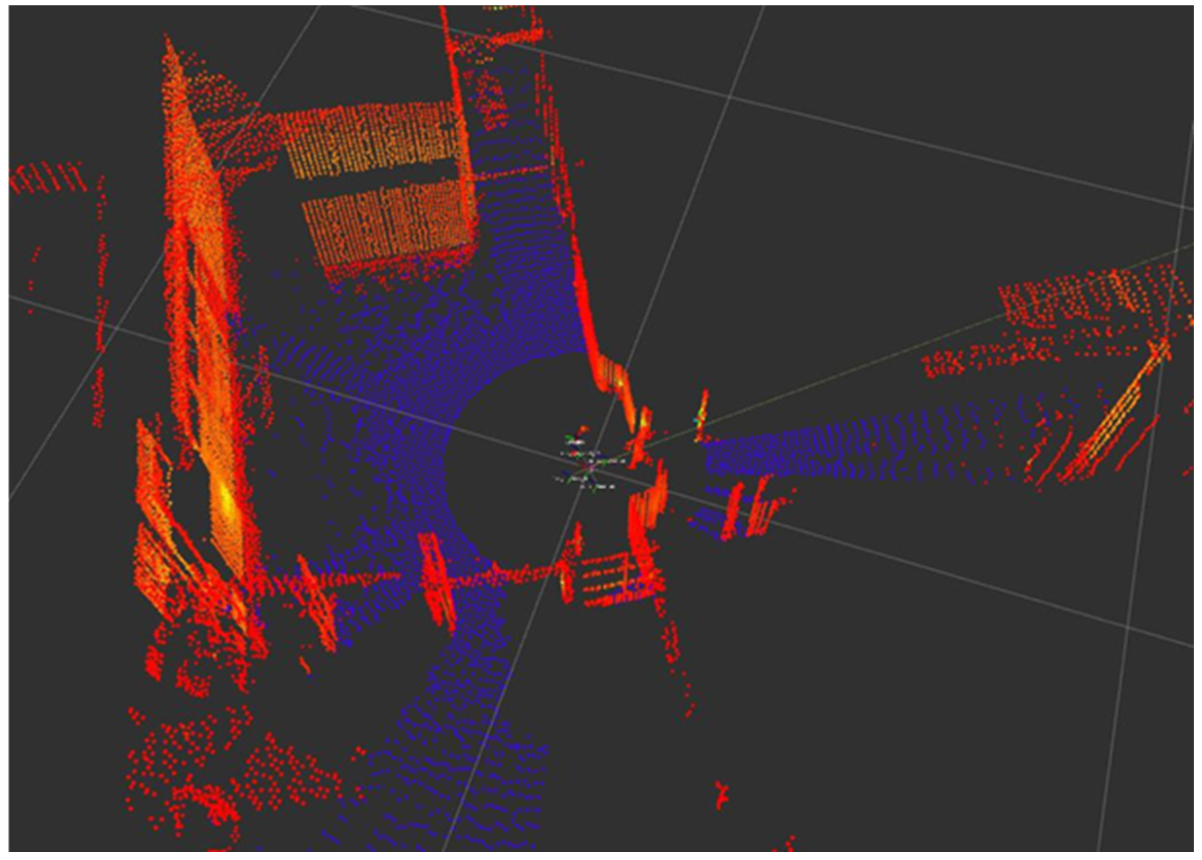
20] In
Figure 5, the points detected by the floor_detection node are shown in blue.
Hdl_graph_slam Node
The estimated odometry (odom) and the estimated floor areas (floor_coeff) are forwarded to the hdl_graph_slam node. In addition, further boundary conditions such as IMU data and GPS can be considered here. These can be activated via corresponding parameters (enable_gps, enable_imu_acc,enable_imu_ori).
2.3. Overall System
The described combination of hard- and software allows for the best possible combination to create precise and high-definition point cloud maps. The employed high-density point cloud LiDAR is fused with information of the RTK-GNSS system to cope with long-term drift that occurs despite the use of state-of-the-art scan matching algorithms.
The mobile platform and its open source-based software suite is easily augmented with algorithms or sensors and perfectly reflect the intended applications of smart logistics, augmented wheelchairs, field robotics surveillance, or household assistance systems.
The overview examination and evaluation of several SLAM methods showed the superiority of the chosen approach in terms of computational and storage load as well as the easy incorporation and use of additional sensors. Theoretical optimality, which can be claimed for competing approaches, is also well proven for graph-based least squares SLAM.
3. Experimental Results
For the evaluation of HDL Graph SLAM with our system, different test scenarios are considered. The test scenarios include the behavior indoors, with a flat floor surface and partially narrow aisles, the behavior outdoors, and the detection of height differences.
The scenarios were chosen to accommodate common situations for the above-mentioned applications, with shadowing of GNSS and repetitiveness of the environment being the main challenges concerning the sensors. The uneven ground plane in the field and the addition of 3D scenarios are part of the second topic addressed to evaluate the overall system.
This chapter first describes the parameter configuration for the tests carried out. This is followed by a presentation of the individual test scenarios and the corresponding results.
3.1. Parameter Configuration
For the evaluation of the SLAM system, all implemented scan matching algorithms are tested. It is shown that FAST_GICP and FAST_VGICP are the most suitable scan matching algorithms for combining HDL Graph SLAM with the Ouster OS1. FAST_GICP and FAST_VGICP do not necessarily require further parameter tuning; thus, they work reliably. Since the literature for NDT registration indicates good results for multi-beam laser scanners, this method is also considered for the results.
3.2. Test Indoor: Hallway of the B-Building
The corridor of the B-building of the Offenburg University of Applied Sciences has dimensions of approximately 40 × 35 m. It is assumed that the floor is flat, and the walls are at right angles to each other. The corridor has many window fronts so that parts of the inner courtyard are also covered by the laser scanner. Laser distance measurements through window glass can result in non-reproducible measurements or reduced accuracy. This is because glass can either cause reflection, or the laser beam is refracted in such a way that it changes its angle or direction [
35]. Furthermore, due to the sharp curves in the corners of the corridor, there are strong rotations between the individual laser scans. Finally, a loop closure occurs, which has to be detected by the algorithm. The floor plan of the corridor in the B-building with the trajectory is shown in
Figure 6.
For the evaluation of the hdl_graph_slam first, the effect of the floor_detection node is examined. For this purpose, the trajectory of the robot with and without the floor_detection node is determined. The algorithms FAST_GICP, FAST_VGICP (reg_resolution = 2.0) and NDT_OMP (reg_resosolution = 2.0) are used as scan matching methods. The determined elevation trajectory is illustrated in
Figure 7. When the floor constraint is disabled, the height varies between 0.3 and −0.7 m for the FAST_GICP and FAST_ VGICP algorithms. With NDT_OMP, the height gradient drifts to over −10 m.
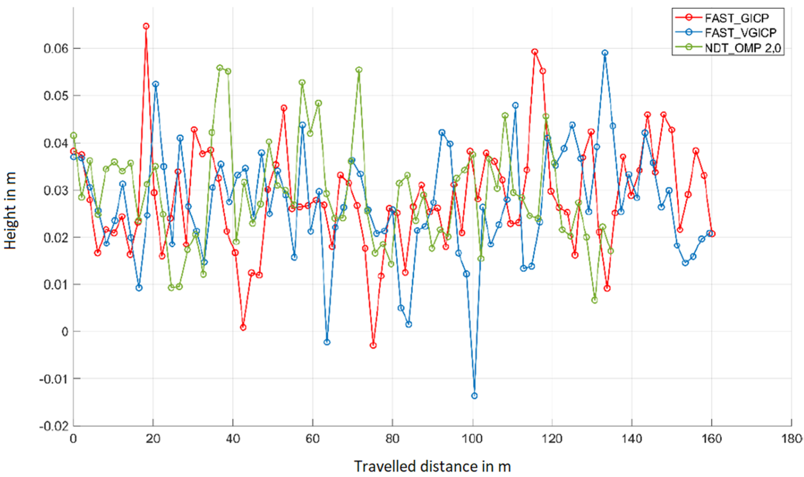
If the ground surface detection is activated, the values of all scans matching algorithms vary only in the range of a few centimeters, as can be seen in
Figure 8. If the floor_detection is not activated, the estimated height course is faulty as well as the trajectory, such that only with the FAST_GICP algorithm a loop closure is detected. Thus, the floor_detection node is essential to be able to determine the optimal trajectory or its optimal height course in the interior of buildings with the hdl_graph_slam.
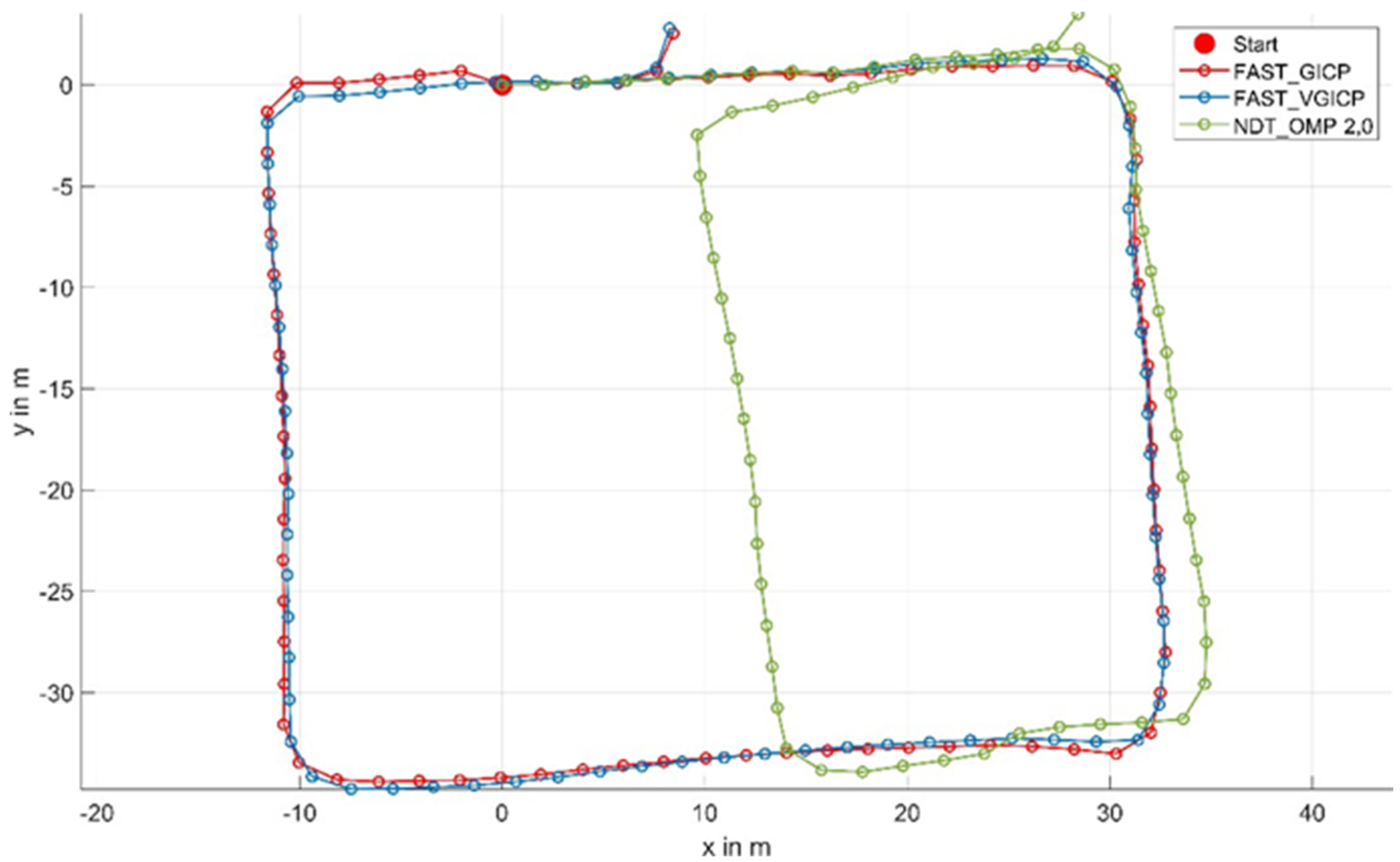
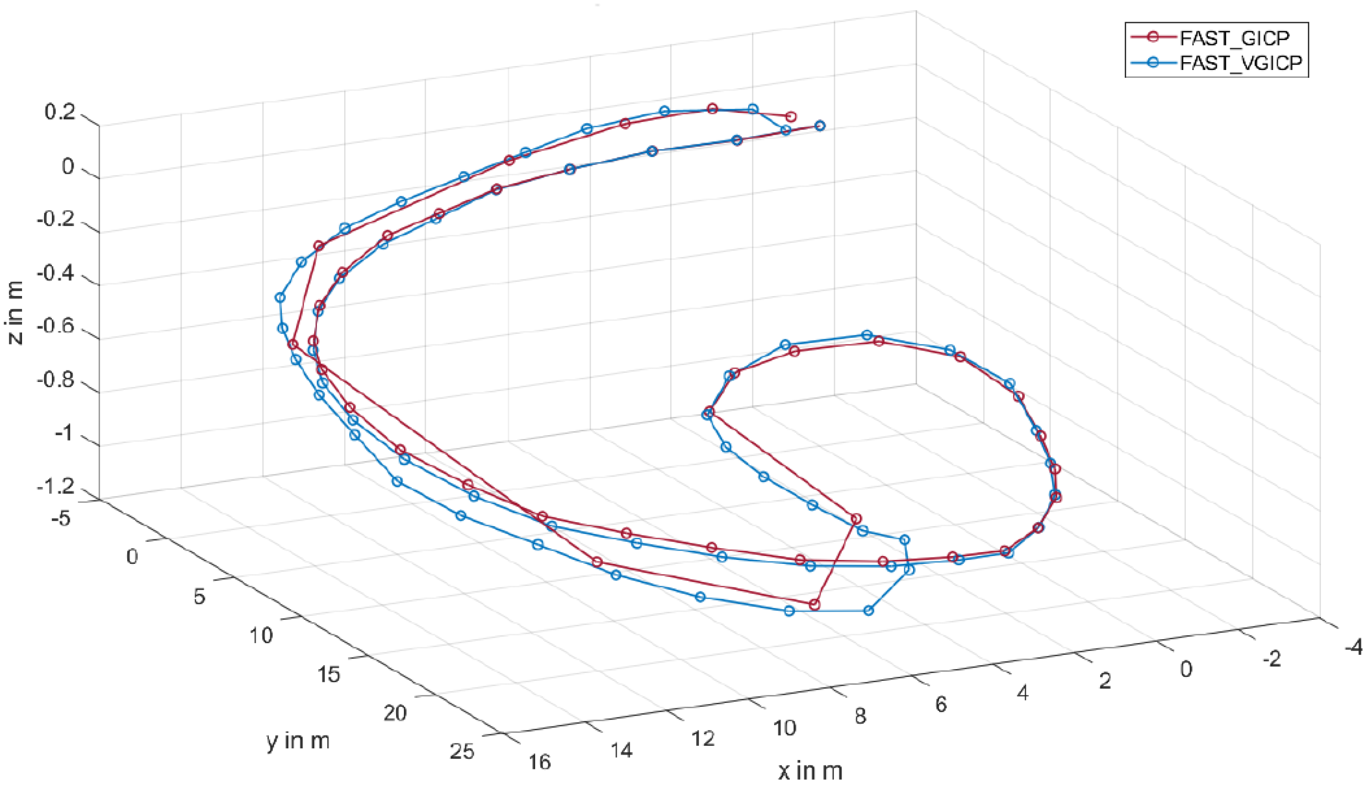
The trajectories determined with the hdl_graph_slam with floor constraint are shown in
Figure 9. The loop closure is detected with all three scan matching algorithms. The trajectory determined with NDT_OMP deviates strongly from the real trajectory in the x-direction despite parameter tuning. The other two algorithms provide almost identical results. Only in the range (−10,0 m) are there slight differences between the two trajectories.
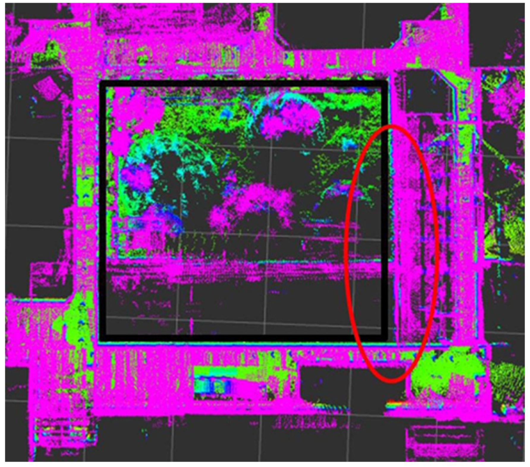
Figure 10 shows the map generated by the hdl_graph_slam (FAST_GICP). To check the accuracy of the generated map, it is examined for its perpendicularity. For this purpose, the detected walls are matched with the rectangle shown in black in the figure. If one assumes that the building is rectangular, it can be seen that the right wall of the created map is not parallel to the drawn rectangle. The black rectangle shows the idealized walls, the red ellipse indicates deviations of the map from the rectangularity. Thus, the map created with hdl_graph_slam is slightly distorted. The use of IMU data as additional boundary conditions did not lead to significant improvements.
3.3. Test Outdoor: Accuracy, Inclination, and Height
For outdoor evaluation, the hdl_graph_slam is tested in the spacious parking lot and on the campus of the university. These two test scenarios are described below.
The Parking Lot of the Offenburg University of Applied Sciences
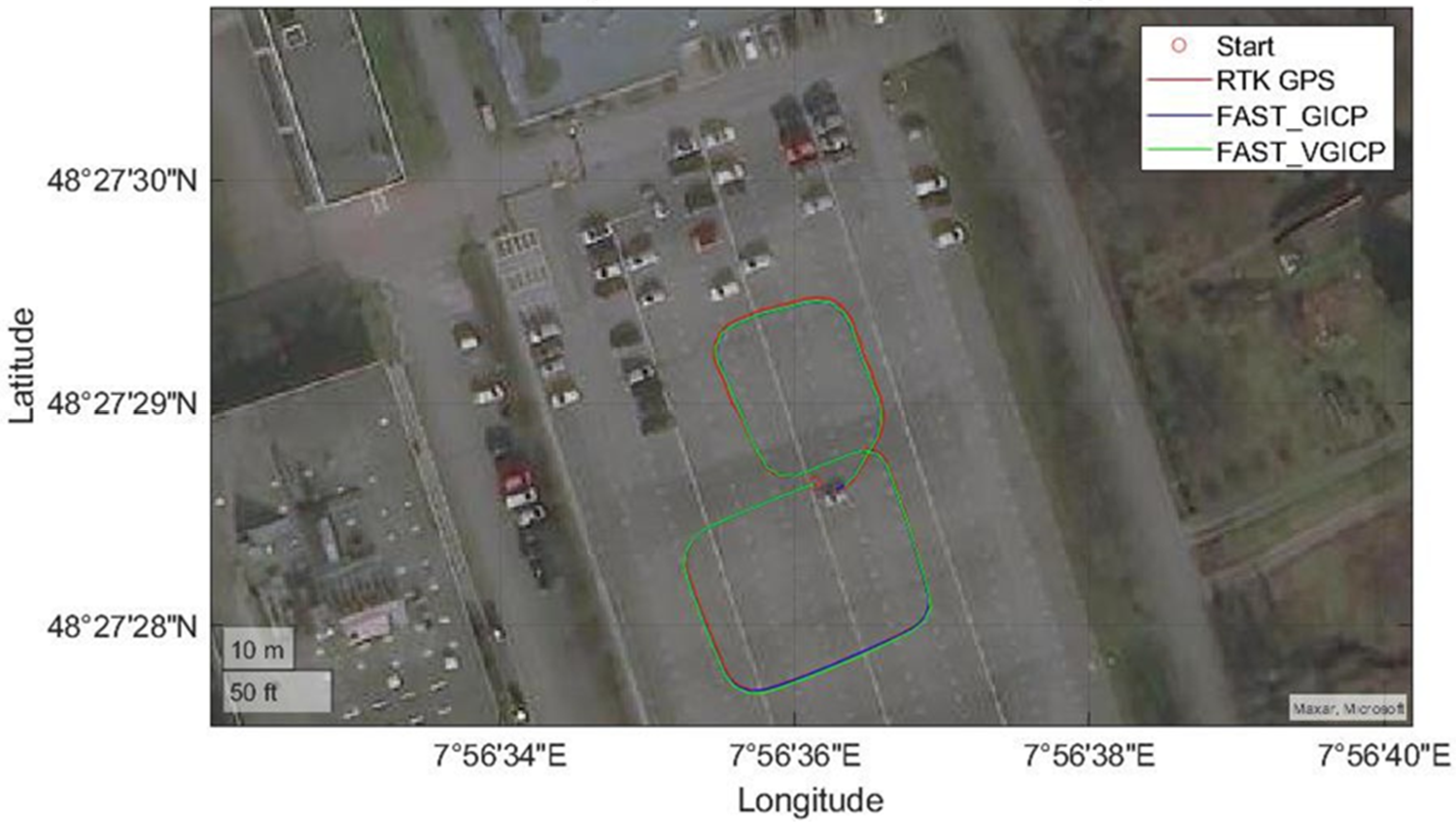
The first outdoor test was recorded in the parking lot of the Offenburg University of Applied Sciences. On the day of the test, the parking lot was sparsely filled with cars, as can be seen in
Figure 11. The parking lot is almost flat and spacious so that only ground surfaces are detected in the immediate vicinity of the Husky robot, and trees and buildings can be detected by the LiDAR sensor from a distance of approximately 40 m. The LiDAR sensor is also able to measure the distance from the parking lot. As a ground truth (reference), the trajectory was also determined using an RTK GPS. For this purpose, the base station was calibrated at the position of the car at the starting point. The RTK GPS can achieve an accuracy of 2 cm when measuring the base station. The total distance of the trajectory is 180 m with a duration of 223 s.
For verification, different scan matching methods for odometry determination are tested again. As in the indoor area, FAST_GICP and FAST_VGICP were shown to be the most suitable for this application. While the hdl_graph_slam with NDT_OMP deviates significantly from the ground truth up to the first loop closure; the deviation of the hdl_graph_slam with the other two algorithms is at a maximum of 20 cm. After the first loop closure, the deviation with all scan matching algorithms is reduced to 2 cm. In the second loop, the deviation with NDT_OMP is up to 3 m but reduces again to a maximum of 1 m at the second loop closure. With FAST_GICP and FAST_VGICP, the deviation is at most 50 cm and reduces again at the loop closure at the end to at most 20 cm. The loop closures found by hdl_graph_slam can be seen on the right side in
Figure 12.
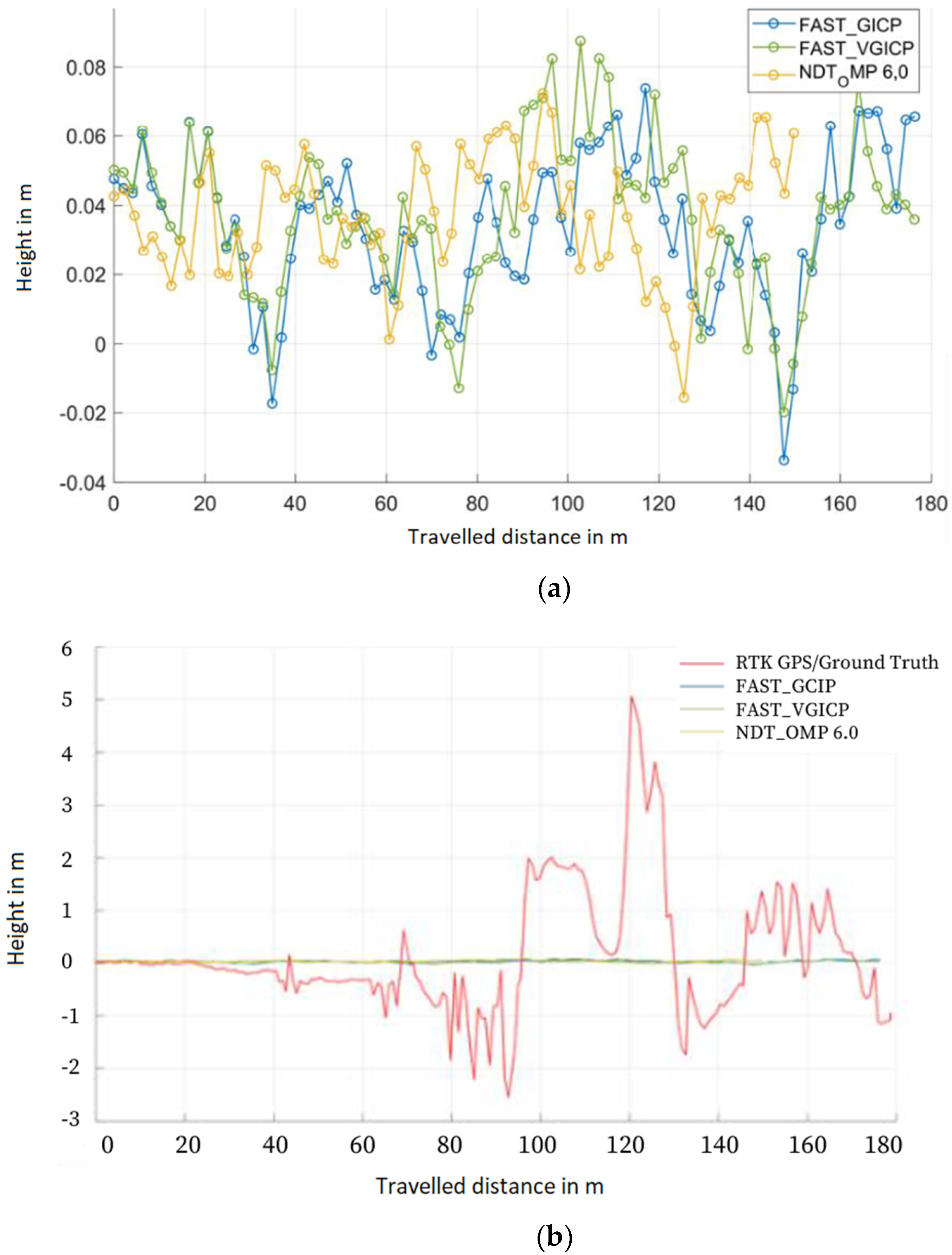
In addition to the trajectory, the elevation profile is also checked. Here, the RTK GPS cannot be used as a reference because its elevation values fluctuate by several meters (
Figure 13a), and this is a flat parking lot. The values of the hdl_graph_slam only vary by ±5 cm. To drain the rainwater, the parking lot is sloped toward a kind of gutter, which represents the low point of the parking lot. In
Figure 12, this is indicated by the red circles. Looking at the elevation of the trajectories, the low point is reached after 34.95 m, which corresponds to the center of the left red circle. The same applies to the right red circle. Due to this, the determined height course is quite plausible but cannot be checked further.
Campus Offenburg University of Applied Sciences
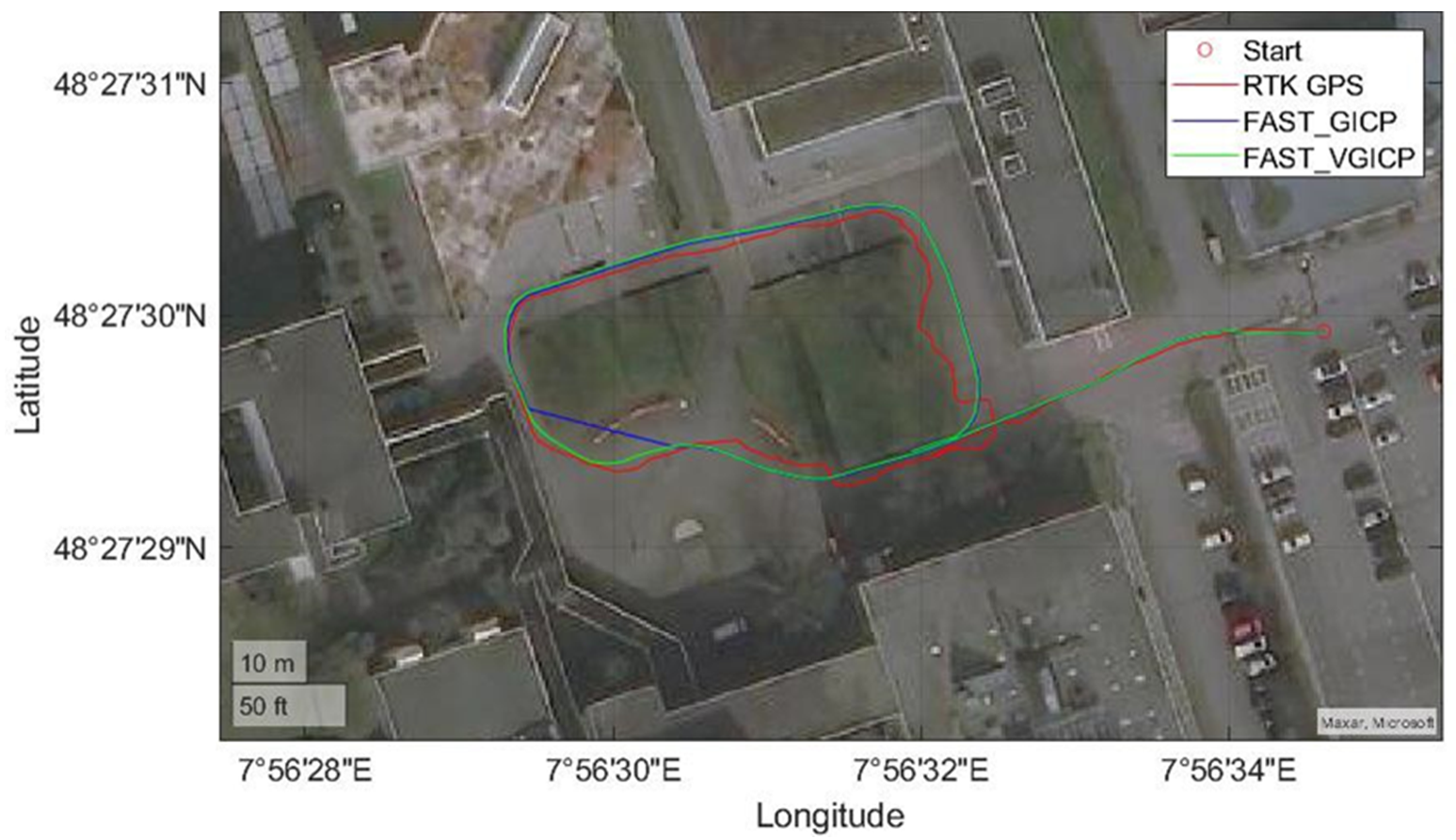
As a second test scenario, a trajectory was recorded with the Husky on the campus of Offenburg University of Applied Sciences, as shown in
Figure 14. There are several buildings on the route at different distances, some of which have large glass fronts. Furthermore, there are many trees on the campus. The ground is also flat in this scenario. Due to the shadowing of the buildings, the trajectory determined by the RTK GPS (see the red trajectory,
Figure 14) was distorted. Therefore, the RTK GPS cannot be used as ground truth.
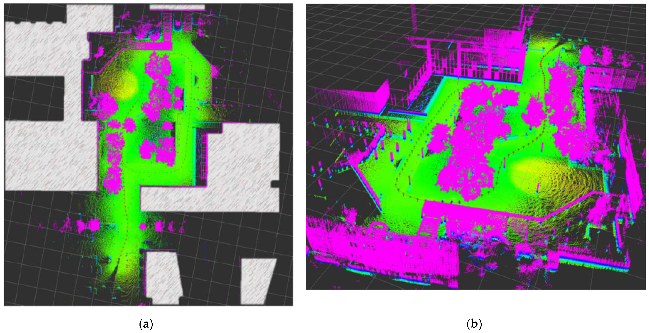
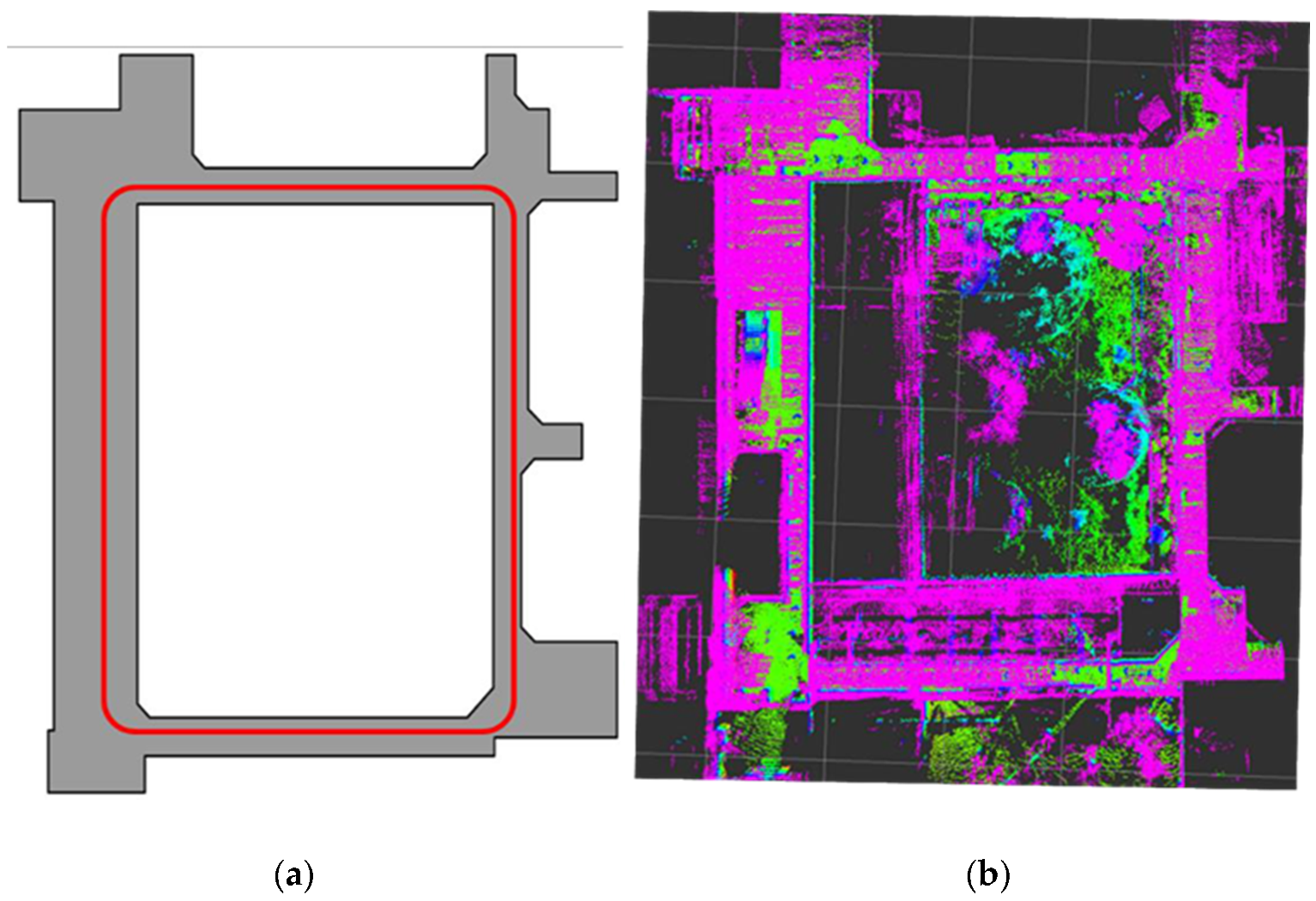
Instead, in this test scenario the created map is compared with the map from the Geoportal BW by superimposing it over the map created with hdl_graph_slam (see
Figure 15). This shows that the contours of the buildings almost match the map available online. The orientation of the buildings to each other, as well as the dimensions of the generated map, match the reference map.
Incline
The last test scenario checks how well hdl_graph_slam detects gradients. For this purpose, two test scenarios are considered, in which the scan matching algorithms FAST_GICP and FAST_VGICP are used. In addition, the tests are performed once with and once without a floor_detection node.
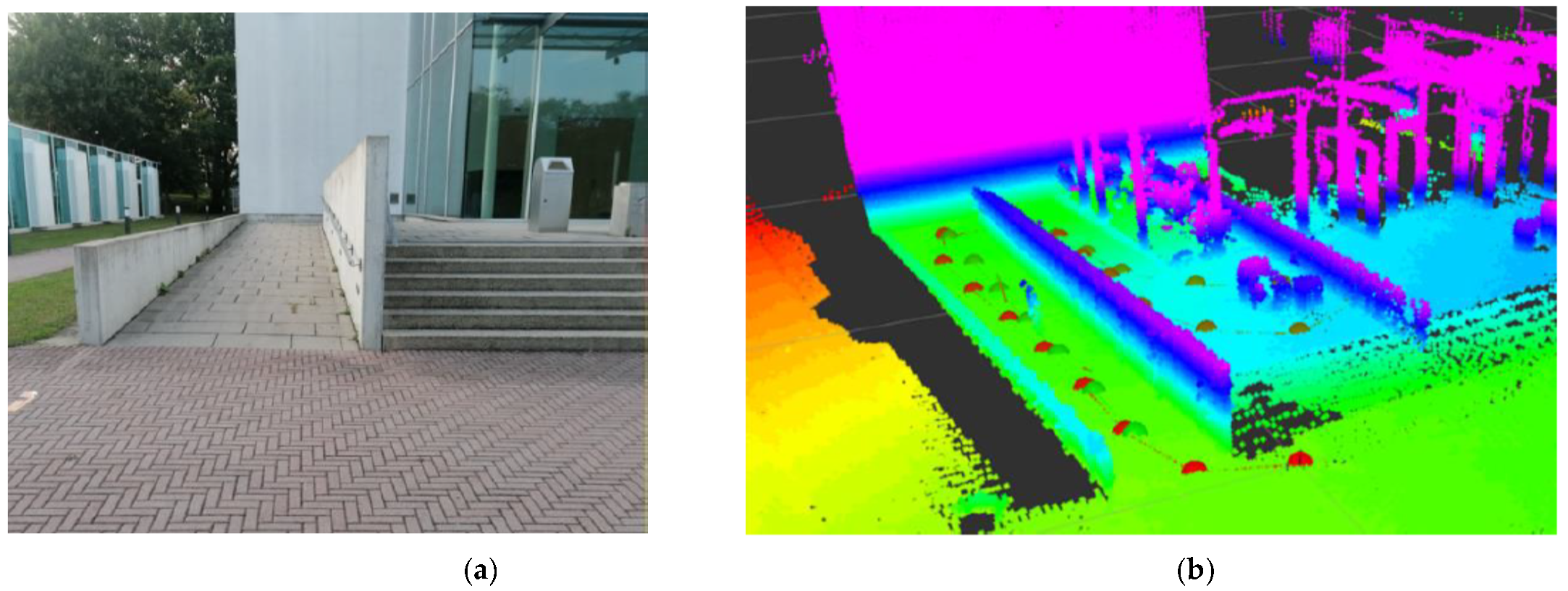
The Entrance Area in Front of the B-Building of the Offenburg University of Applied Sciences
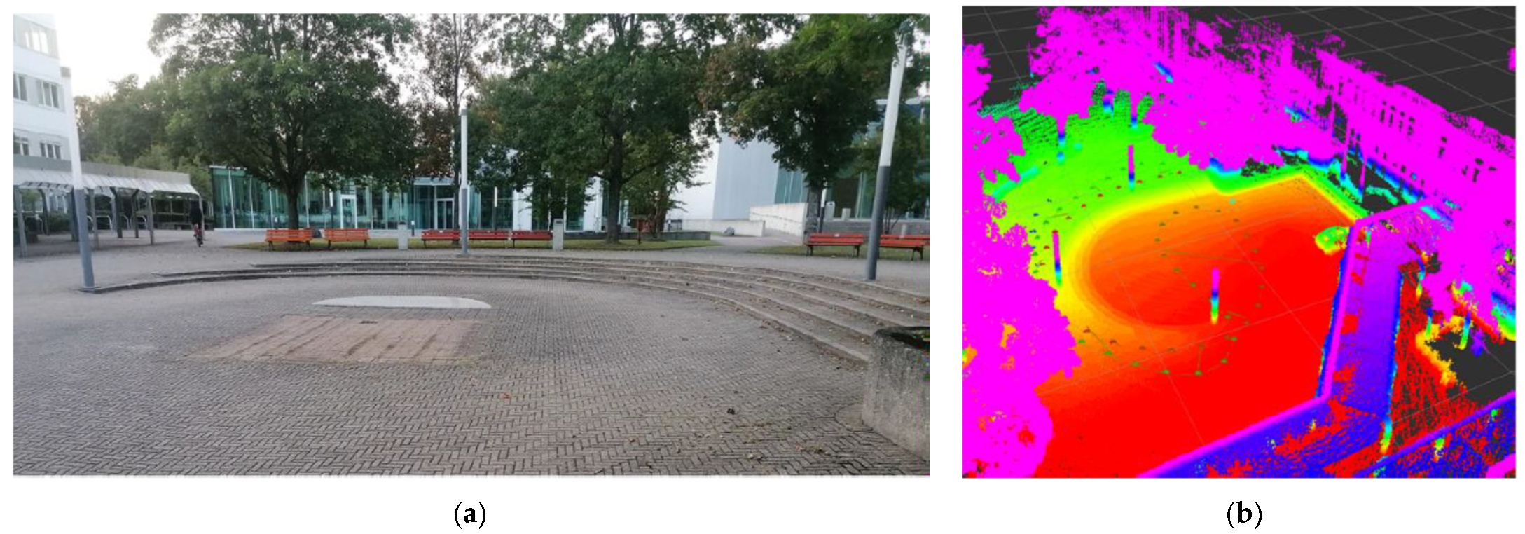
The first test track is shown in
Figure 16. The trajectory driven can be seen on the right side of the figure. This test scenario involves a slowly sloping terrain. The robot started on the right side above the stairs. The robot was then steered in a large loop around the steps, returning to the starting point after one loop. The height difference covered by the stairs is 51 cm.
If the floor_detection node is activated, the height curve shown in
Figure 17 results.
Instead of a decreasing height curve, the height increases by 20 cm while the robot moves downward. The trajectory determined in this way looks correct, but the recorded height profile is incorrect. The same can be seen when activating the floor_detection node on the second test track. This should therefore only be activated for flat surfaces (and otherwise deactivated).
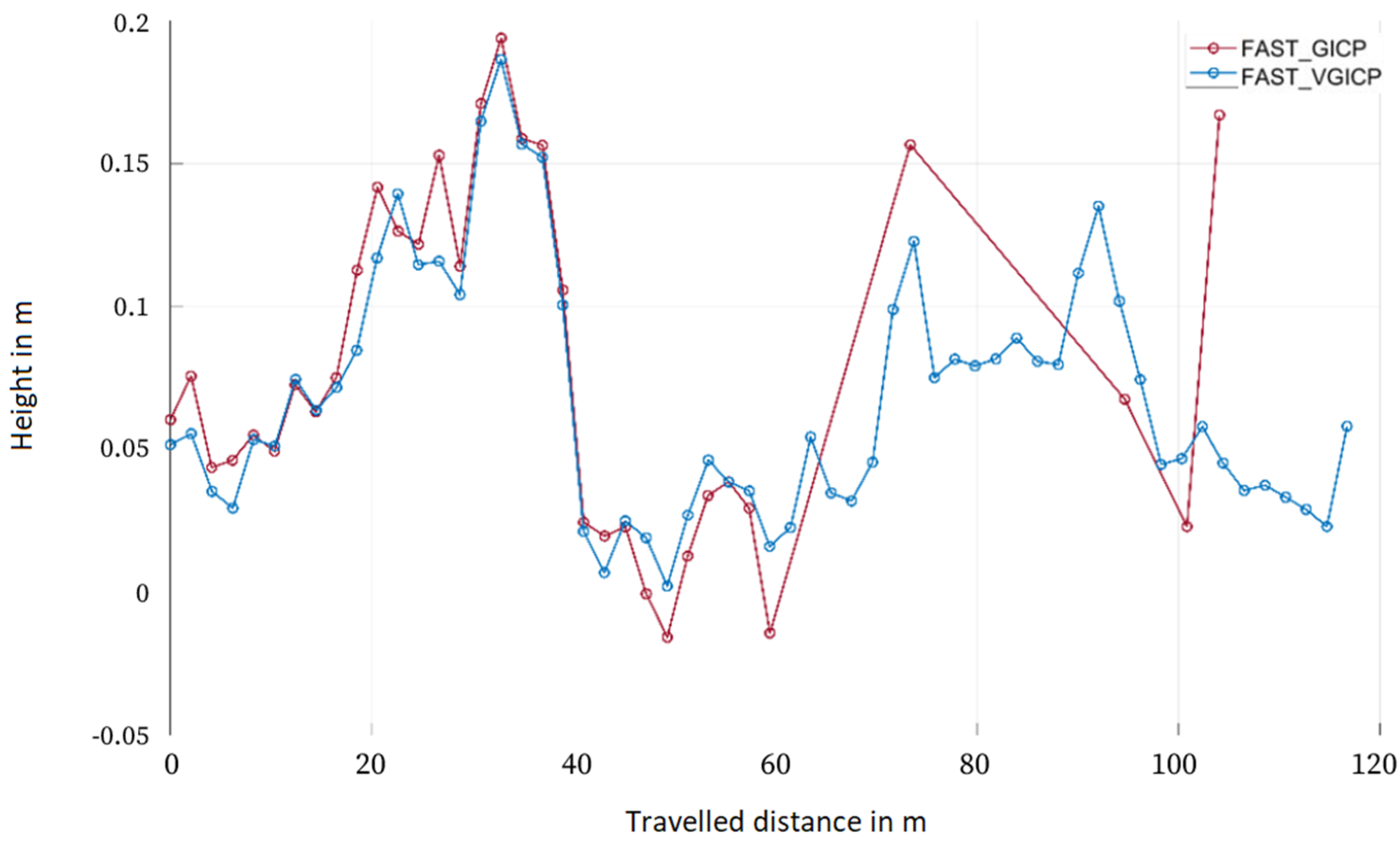
If the floor_detection node is deactivated, the following height trajectory is obtained (
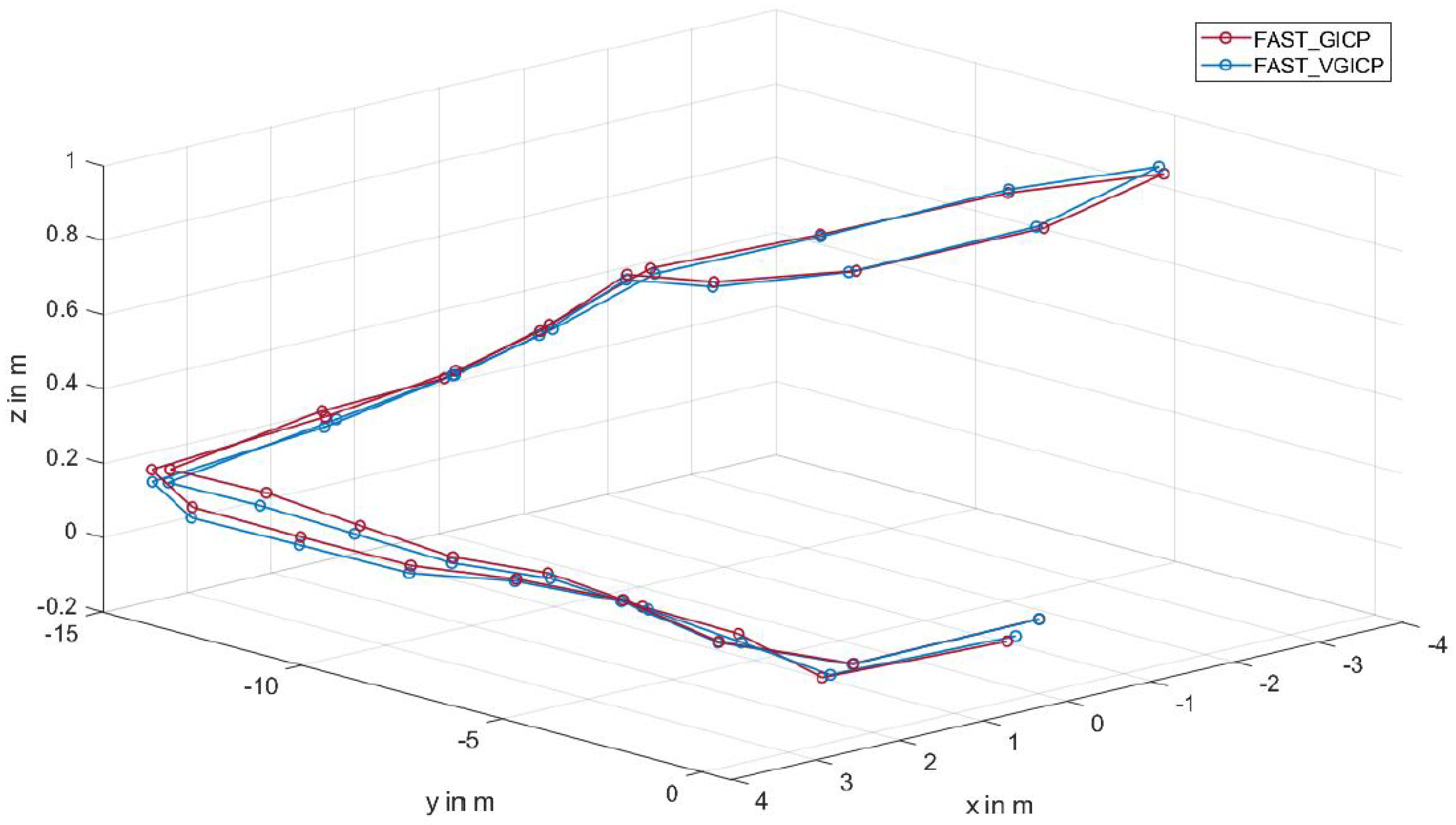
Figure 18). At the height measurement point, the height of the trajectory is −57 cm, while the actual measured height is −51 cm, resulting in a deviation of 6 cm. Once the robot has returned to its starting position, the height values are again 0 cm. In addition, the determined gradient decreases continuously. Thus, the hdl_graph_slam delivers good results with FAST_GICP as well as with FAST_VGICP.
Wheelchair Ramp in Front of the D-building
The wheelchair ramp in front of the D-building of the Offenburg University of Applied Sciences is used as the second test track. This overcomes a height of 88 cm and is shown in the following figure (
Figure 19).
The highest point of the trajectory determined by hdl_graph_slam is at 90 cm (FAST_VGICP) or 88 cm (FAST_GICP), which corresponds to the measured altitude. However, the height values of the loop, which was run on the actual flat altitude, vary between 70 and 90 cm (
Figure 20). In addition, the wheelchair run is a continuous slope.
Looking at the trajectory estimated by hdl_graph_slam, it has different slopes before and after the curve. Nevertheless, the trajectory reaches the initial level again at the return.
3.4. Experimental Results—Core Findings
The conducted experiments with our system clearly indicate the usefulness and capability of the autonomous robot for the considered applications. Although, some key findings need to be exclusively addressed: The system shows great performance and reliability for indoor scenarios on the condition that the floor plane is estimated. Otherwise, the densely collected points rather deviate from the resulting map.
The floor plane estimation is also crucial for outdoor applications that fit into this scenario, such as surveillance of parking lots or driving in an urban environment and concrete pave ways. Nonetheless, it must be remarked that the floor plane must be deactivated, for example, in a kind of mission planning scenario, when several levels of height, ramps, or uneven terrain are traveled.
Under the condition of making use of the environment for loop closures, the overall accuracy is excellent, showing deviations under 10 cm for long ways traveled and height accuracy down to 2 cm. This is especially important for scenarios where shadowing of the GNSS occurs or when height has to be taken explicitly into account. Here, our system clearly outperforms the RTK-GPS taken as a reference.
As a drawback, accuracy deteriorates when loop closures are not possible. In these scenarios, simpler local odometry and mapping algorithms perform better, giving a smaller error, especially for driving lengths above 200 m.
4. Conclusions
In the last chapter, it has been shown that the hdl_graph_slam in combination with the LiDAR OS1 from Ouster and the scan matching algorithms FAST_GICP and FAST_VGICP achieve good mapping results.
In the indoor domain, the floor_detection node should be used to improve the accuracy of the estimated trajectory, especially in terms of elevation. The dimensions of the generated map in the indoor area were correct except for one wall that was not detected perpendicularly.
In the outdoor area, the results were also good; thus, the trajectory determined with hdl_graph_slam almost matched the ground truth trajectory of the RTK GPS. The generated map of the university campus was also satisfactory, as hardly any distortions could be detected.
The slope tests showed that even to detect only minor elevation changes, the floor_detection node should be deactivated. The absolute height difference could be determined precisely with hdl_graph_slam. Thus, the determined height for the wheelchair walks exactly matched the reference, deviating by only 6 cm in the former test scenario. However, the intervening slope of the wheelchair ramp only slightly matched the actual one.
In summary, the hdl_graph_slam is well suited for mapping an environment using Ouster’s 3D LiDAR and thus can be used in many autonomous mobile systems. The evaluated results related to positioning performance using LiDAR can be useful baseline work to further improve positioning performance using LiDAR-based SLAM systems.
Author Contributions
Conceptualization, S.H. and M.B.M.; methodology, S.H. and M.O.; software, M.O.; validation, S.H; investigation, S.H., M.B.M. and M.O.; resources, S.H.; writing—original draft preparation, S.H. and M.O.; writing—review and editing, S.H. and M.B.M.; visualization, S.H. and M.O.; funding acquisition, M.B.M. All authors have read and agreed to the published version of the manuscript.
Funding
This research is supported by the Bulgarian National Science Fund in the scope of the project “Exploration the application of statistics and machine learning in electronics” under contract number KΠ-06-H42/1.
Institutional Review Board Statement
Not applicable.
Informed Consent Statement
Not applicable.
Data Availability Statement
Data are contained within the article.
Acknowledgments
The authors would like to thank the Research and Development Sector of the Technical University of Sofia for its financial support.
Conflicts of Interest
The authors declare no conflict of interest.
References
- Durrant-Whyte, H.; Bailey, T. Simultaneous Localisation and Mapping (SLAM): Part I The Essential Algorithms. Robot. Autom. Mag. 2006, 2, 1–9. [Google Scholar]
- Ivanova, M.; Petkova, P.; Petkov, P. Machine Learning and Fuzzy Logic in Electronics: Applying Intelligence in Practice. Electronics 2021, 10, 2878. [Google Scholar] [CrossRef]
- Hensel, S.; Marinov, M.B.; Kehret, C.; Stefanova-Pavlova, M. Experimental Set-up for Evaluation of Algorithms for Simultaneous Localization and Mapping. In Systems, Software and Services Process Improvement; EuroSPI 2020, Communications in Computer and Information Science; Springer Nature Switzerland AG: Cham, Switzerland, 2020; Volume 1251, pp. 433–444. [Google Scholar]
- Cadena, C.; Carlone, L.; Carrillo, H.; Latif, Y.; Scaramuzza, D.; Neira, J.; Reid, I.; Leonard, J. Past, Present, and Future of Simultaneous Localization and Mapping: Towards the Robust-Perception Age. IEEE Trans. Robot. 2016, 32, 1309–1332. [Google Scholar] [CrossRef]
- Hess, W.; Kohler, D.; Rapp, H.; Andor, D. Real-Time Loop Closure in 2D LIDAR SLAM. In Proceedings of the IEEE International Conference on Robotics and Automation (ICRA), Stockholm, Sweden, 16–21 May 2016. [Google Scholar]
- Grisetti, G.; Kümmerle, R.; Stachniss, C.; Burgard, W. A Tutorial on Graph-Based SLAM. IEEE Intell. Transp. Syst. Mag. 2010, 2, 31–43. [Google Scholar] [CrossRef]
- Stateczny, A.; Specht, C.; Specht, M.; Brčić, D.; Jugović, A.; Widźgowski, S.; Wiśniewska, M.; Lewicka, O. Study on the Positioning Accuracy of GNSS/INS Systems Supported by DGPS and RTK Receivers for Hydrographic Surveys. Energies 2021, 14, 7413. [Google Scholar] [CrossRef]
- Specht, M.; Stateczny, A.; Specht, C.; Widźgowski, S.; Lewicka, O.; Wiśniewska, M. Concept of an Innovative Autonomous Unmanned System for Bathymetric Monitoring of Shallow Waterbodies (INNOBAT System). Energies 2021, 14, 5370. [Google Scholar] [CrossRef]
- Zhang, J.; Singh, S. LOAM: Lidar Odometry and Mapping in Real-time. In Proceedings of the Robotics: Science and Systems, Berkeley, CA, USA; 2014. [Google Scholar]
- Weber, H. Funktionsweise und Varianten von LiDAR-Sensoren. Available online: https://cdn.sick.com/media/docs/5/25/425/whitepaper_lidar_de_im0079425.pdf (accessed on 20 October 2021).
- Maksymova, I.; Steger, C.; Druml, N. Review of LiDAR Sensor Data Acquisition and Compression for Automotive Applications. Proceedings 2018, 2, 852. [Google Scholar]
- Koide, K.; Miura, J.E.M. A portable three-dimensional LIDAR-based system for long-term and wide-area people behavior measurement. Int. J. Adv. Robot. Syst. 2019, 16, 1–16. [Google Scholar] [CrossRef]
- Burdziakowski, P. Increasing the Geometrical and Interpretation Quality of Unmanned Aerial Vehicle Photogrammetry Products using Super-resolution Algorithms. Remote Sens. 2020, 12, 810. [Google Scholar] [CrossRef]
- Koide, K.; Yokozuka, M.; Oishi, S.; Banno, A. Voxelized GICP for Fast and Accurate 3D Point Cloud Registration. In Proceedings of the 2021 IEEE International Conference on Robotics and Automation (ICRA), Xi’an, China, 30 May–5 June 2021. [Google Scholar]
- Hensel, S.; Marinov, M.; Obert, M.; Trendafilov, D. Design and Implementation of a LIDAR Based Range Sensor System. Complex Control. Syst. 2022, 4, 16–21. [Google Scholar]
- Ouster. Ouster OS1: Mid-Range High-Resolution Imaging Lidar. Available online: https://ouster.com/products/os1-lidar-sensor/. (accessed on 20 October 2021).
- Obert, M. Inbetriebnahme und Evaluierung des hdl_graph_slam mit einem 128 Zeilen Ouster LiDAR-Sensor auf der Husky Roboterplattform von Clearpath; Hochschule Offenburg: Offenburg, Germany, 2021. [Google Scholar]
- Bakuła, M.; Przestrzelski, P.; Kaźmierczak, R. Reliable technology of centimeter GPS/GLONASS surveying in forest environments. IEEE Trans. Geosci. Remote Sens. 2015, 53, 1029–1038. [Google Scholar] [CrossRef]
- Specht, C.; Specht, M.; Dabrowski, P. Comparative Analysis of Active Geodetic Networks in Poland. In Proceedings of the 17th International Multidisciplinary Scientific GeoConference (SGEM 2017), Albena, Bulgaria, 29 June–5 July 2017. [Google Scholar]
- Kupitz, C. Inbetriebnahme und Verifizierung eines Kalman Filter zur Lagebestimmung des Clearpath Robotics Husky A200; Technical report; Department for Electrical Engineering, University of Applied Sciences Offenburg: Offenburg, Germany, 2021. [Google Scholar]
- Jelavic, E. ETH Zürich: Programming for Robotics, Introduction to ROS. Available online: https://rsl.ethz.ch/education-students/lectures/ros.html (accessed on 21 July 2022).
- Blasdel. About ROS.Version: 2020. Available online: https://www.ros.org/about-ros/ (accessed on 21 July 2022).
- Quigley, M.; Conley, K.; Gerkey, B.; Faust, J.; Foote, T.; Leibs, J.; Wheeler, R.; Ng, A.Y. ROS: An open-source Robot Operating System. In ICRA Workshop on Open Source Software. ICRA Workshop on Open Source Software, Kobe, Japan, 12–17 May 2009. [Google Scholar]
- Besl, P.J.; McKay, N.D. A method for registration of 3-D shapes. IEEE Trans. Pattern Anal. Mach. Intell. 1992, 14, 239–256. [Google Scholar] [CrossRef]
- Biber, P.; Strasser, W. The normal distributions transform: A new approach to laser scan matching. In Proceedings of the 2003 IEEE/RSJ International Conference on Intelligent Robots and Systems (IROS 2003), Las Vegas, NV, USA, 27–31 October 2003. [Google Scholar]
- Konolige, K.; Nüchter, A. Springer Handbook of Robotics; Siciliano, B., Khatib, O., Eds.; Springer: Berlin/Heidelberg, Germany, 2016. [Google Scholar]
- Montemerlo, M.; Thrun, S. Simultaneous localization and mapping with unknown data association using FastSLAM. In Proceedings of the 2003 IEEE International Conference on Robotics and Automation (Cat. No.03CH37422), Taipei, Taiwan, 14–19 September 2003. [Google Scholar]
- Carlone, L.; Calafiore, G.C.; Tommolillo, C.; Dellaert, F. Planar Pose Graph Optimization: Duality, Optimal Solutions, and Verification. IEEE Trans. Robot. 2016, 32, 545–565. [Google Scholar] [CrossRef]
- Dellaert, F. Factor Graphs: Exploiting Structure in Robotics. Annu. Rev. Control. Robot. Auton. Syst. 2021, 4, 141–166. [Google Scholar] [CrossRef]
- Droeschel, D.; Nieuwenhuisen, M.; Beul, M.; Stueckler, J.; Holz, D.; Behnke, S. Multi-Layered Mapping and Navigation for Autonomous Micro Aerial Vehicles. J. Field Robot. 2016, 33, 451–475. [Google Scholar] [CrossRef]
- Engel, J.; Schöps, T.; Cremers, D. LSD-SLAM: Large-Scale Direct Monocular SLAM. Lect. Notes Comput. Sci. 2014, 8690, 834–849. [Google Scholar]
- Zhang, J.; Singh, S. Laser–visual–inertial odometry and mapping with high robustness and low drift. J. Field Robot. 2018, 35, 1242–1264. [Google Scholar] [CrossRef]
- Wan, G.; Yang, X.; Cai, R.; Li, H. Robust and Precise Vehicle Localization Based on Multi-Sensor Fusion in Diverse City Scenes. In Proceedings of the 2018 IEEE International Conference on Robotics and Automation (ICRA), Brisbane, Australia, 21–26 May 2018. [Google Scholar]
- Available online: https://github.com/koide3,koide3/hdl_graph_slam,2021 (accessed on 22 April 2022).
- Ali, H.; Ahmed, B.; Paar, G. Robust Window Detection from 3D Laser Scanner Data. In Proceedings of the 2008 Congress on Image and Signal Processing, Sanya, China, 27–30 May 2008. [Google Scholar]
Figure 1.
Up: Horizontal distance between two laser beams as a function of distance. Down: Vertical field of view as a function of distance (100 m).
Figure 1.
Up: Horizontal distance between two laser beams as a function of distance. Down: Vertical field of view as a function of distance (100 m).
Figure 2.
The hardware structure of the robot platform (based on [
20]).
Figure 2.
The hardware structure of the robot platform (based on [
20]).
Figure 3.
ICP algorithm: (a) flowchart; (b) basic idea.
Figure 3.
ICP algorithm: (a) flowchart; (b) basic idea.
Figure 4.
Overview of the nodes of the hdl_graph_slam [
34].
Figure 4.
Overview of the nodes of the hdl_graph_slam [
34].
Figure 5.
Laser scan in the corridor of the B-building of the Offenburg University of Applied Sciences. (Blue: floor area detected by the floor_detection node, red: remaining laser scan points).
Figure 5.
Laser scan in the corridor of the B-building of the Offenburg University of Applied Sciences. (Blue: floor area detected by the floor_detection node, red: remaining laser scan points).
Figure 6.
(a) Trajectory and floor plan of the corridor in the B-building of the University of Applied Sciences Offenburg, Germany. (b) Map created with hdl_graph_slam.
Figure 6.
(a) Trajectory and floor plan of the corridor in the B-building of the University of Applied Sciences Offenburg, Germany. (b) Map created with hdl_graph_slam.
Figure 7.
Height profile as a function of the distance covered in the corridor of the B-building of Offenburg University with and without floor constraint.
Figure 7.
Height profile as a function of the distance covered in the corridor of the B-building of Offenburg University with and without floor constraint.
Figure 8.
Height profile as a function of the distance covered in the corridor of the B-building of the Offenburg University of Applied Sciences with floor detection.
Figure 8.
Height profile as a function of the distance covered in the corridor of the B-building of the Offenburg University of Applied Sciences with floor detection.
Figure 9.
Trajectories of the hdl_graph_slam in the corridor of the B-building of the Offenburg University of Applied Sciences.
Figure 9.
Trajectories of the hdl_graph_slam in the corridor of the B-building of the Offenburg University of Applied Sciences.
Figure 10.
Map of the corridor in the B-building of the University of Applied Sciences Offenburg created with hdl_graph_slam (FAST_GICP).
Figure 10.
Map of the corridor in the B-building of the University of Applied Sciences Offenburg created with hdl_graph_slam (FAST_GICP).
Figure 11.
Trajectories of the different scan matching methods (FAST_GICP, FAST_VGICP, and RTK GPS as ground truth) on the parking lot of the Offenburg University of Applied Sciences.
Figure 11.
Trajectories of the different scan matching methods (FAST_GICP, FAST_VGICP, and RTK GPS as ground truth) on the parking lot of the Offenburg University of Applied Sciences.
Figure 12.
Left: Trajectories of the different scan matching methods (FAST_GICP, FAST_VGICP, NDT_OMP, and RTK GPS as ground truth) on the parking lot of the University of Applied Sciences Offenburg. Right: Trajectory with four loop closures found.
Figure 12.
Left: Trajectories of the different scan matching methods (FAST_GICP, FAST_VGICP, NDT_OMP, and RTK GPS as ground truth) on the parking lot of the University of Applied Sciences Offenburg. Right: Trajectory with four loop closures found.
Figure 13.
(a) Height course of the trajectory of the different scan matching methods (FAST_GICP, FAST_VGICP, and NDT_OMP) on the parking lot of the University of Applied Sciences Offenburg. (b) Elevation trajectory of the RTK GPS (red).
Figure 13.
(a) Height course of the trajectory of the different scan matching methods (FAST_GICP, FAST_VGICP, and NDT_OMP) on the parking lot of the University of Applied Sciences Offenburg. (b) Elevation trajectory of the RTK GPS (red).
Figure 14.
The trajectory on the campus of the Offenburg University of Applied Sciences.
Figure 14.
The trajectory on the campus of the Offenburg University of Applied Sciences.
Figure 15.
(a) Comparison of the map created using hdl_graph_slam (FAST_GICP) with the map of the Geoportal BW. (b) Map of the Offenburg campus created with hdl_graph_slam (FAST_GICP).
Figure 15.
(a) Comparison of the map created using hdl_graph_slam (FAST_GICP) with the map of the Geoportal BW. (b) Map of the Offenburg campus created with hdl_graph_slam (FAST_GICP).
Figure 16.
(a) Test track. (b) Map of the entrance area of the B-building created using hdl_graph_slam.
Figure 16.
(a) Test track. (b) Map of the entrance area of the B-building created using hdl_graph_slam.
Figure 17.
Height course of the trajectory determined by hdl_graph_slam with the activated floor_detection node.
Figure 17.
Height course of the trajectory determined by hdl_graph_slam with the activated floor_detection node.
Figure 18.
Height course of the trajectory determined by hdl_graph_slam with deactivated floor_detection node.
Figure 18.
Height course of the trajectory determined by hdl_graph_slam with deactivated floor_detection node.
Figure 19.
(a) Test track. (b) Map created using hdl_graph_slam from the wheelchair ramp of the D-building.
Figure 19.
(a) Test track. (b) Map created using hdl_graph_slam from the wheelchair ramp of the D-building.
Figure 20.
Height course of the trajectory determined by hdl_graph_slam with deactivated floor_detection node.
Figure 20.
Height course of the trajectory determined by hdl_graph_slam with deactivated floor_detection node.
Table 1.
The distance of the measuring points depends on the distance [
17].
Table 1.
The distance of the measuring points depends on the distance [
17].
| Alignment | Resolution,
Points | Field of View, ° | Angle between
Two Beams, ° | Distance, m | Raster Size, cm |
|---|
| Vertical | 128 | 45 | 0.35 | 100 | 61.36 |
| 10 | 6.14 |
| Horizontal | 512 | 360 | 0.70 | 100 | 122.72 |
| 10 | 12.27 |
| 1028 | 360 | 0.35 | 100 | 61.12 |
| 10 | 6.11 |
| 2048 | 360 | 0.18 | 100 | 30.68 |
| 10 | 3.07 |
| Publisher’s Note: MDPI stays neutral with regard to jurisdictional claims in published maps and institutional affiliations. |
© 2022 by the authors. Licensee MDPI, Basel, Switzerland. This article is an open access article distributed under the terms and conditions of the Creative Commons Attribution (CC BY) license (https://creativecommons.org/licenses/by/4.0/).


