Abstract
This article deals with the use of contactless measurement with a high-resolution imaging device during tensile testing of materials in a universal tearing machine (UTM). Setting the material parameters in tensile testing is based on changes in the geometrical properties of the sample being tested. In this article, authors propose the method and system for automated measuring the height, width, and crack occurrence during tensile testing. The system is also able to predict the location of crack occurrence. The proposed method is based on selected algorithms of image analysis, feature extraction, and template matching. Our video extensometry, working with common inspection cameras operating in visible range, can be an alternative method to expensive laser extensometry machines. The motivation of our work was to develop an automated measurement system for use in a UTM.
1. Introduction
Tensile testing is a destructive way to determine the mechanical properties, yield strength, and flexibility of materials. It calculates the amount of force needed to break a hybrid or plastic specimen, and also how far the specimen must stretch or elongate to achieve that breaking point. Composites are typically subjected to basic tension or flat-sandwich tension testing by standards ISO 527-4, ISO 527-5, ASTM D 638, ASTM D 3039, and ASTM C 297. The tensile modulus is calculated using stress–strain diagrams obtained from these experiments [1].
Tensile testing provides many measurements leading to the determination of selected material parameters, for example (based on ASTM D 3039) ultimate tensile strength (σmax), ultimate tensile strain (ε), modulus of elasticity (E), and Poisson’s ratio (ν). In-plane tensile testing is the most common test for basic composite laminates. Resin-impregnated fiber bundles (“tows”), through-thickness samples (cut from thick lamination portions), and sandwich core material portions are all tensile tested. Alignment is critical for composite testing applications because polymers are anisotropic and often brittle. Anisotropy describes how the material’s properties and strength change based on the direction of applied load or stress. As a result, a composite material’s tensile strength is very high when measured in the direction parallel to the fiber orientation, but substantially lower when tested in any other direction. Surprisingly, the tensile test must have exceptional axial-load–string alignment to estimate maximum tensile strength in the direction parallel to the fiber direction, which is especially important in the aerospace industry, where composites are frequently used in high tensile-stress constructions [1,2].
For ambient, sub-ambient, and high-temperature testing, a variety of proven gripping mechanisms, including manual, pneumatic, and hydraulic actuation, are currently available, with temperatures ranging from 269 to 600 °C. The results of the tests are used to choose the best materials, design parts that can bear application stresses, and perform important quality control checks on the materials [3].
The tensile test is among the most important tensile testing, and because of its assumption, simplicity, and efficiency, it is the most extensively used and recognized test technique for assessing the mechanical characteristics of mostly metallic materials. It also has the benefit of being able to fracture any material while still following the mathematical similarity law [4].
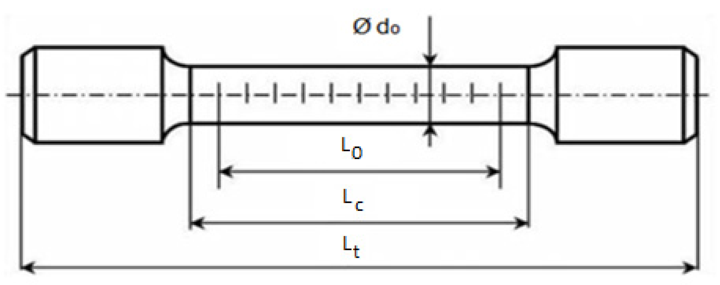
It entails attaching a clean testing object with a basic form (usually circular and rectangular pass) to the tearing machine’s jaws (Figure 1).
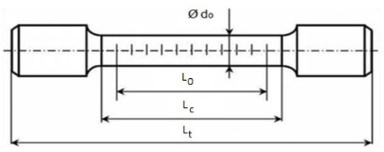
Figure 1.
Sample under test and its typical dimensions, Lc is parallel length, L0 is original gauge length, Lt is total length of tested piece, and d0 is diameter of sample.
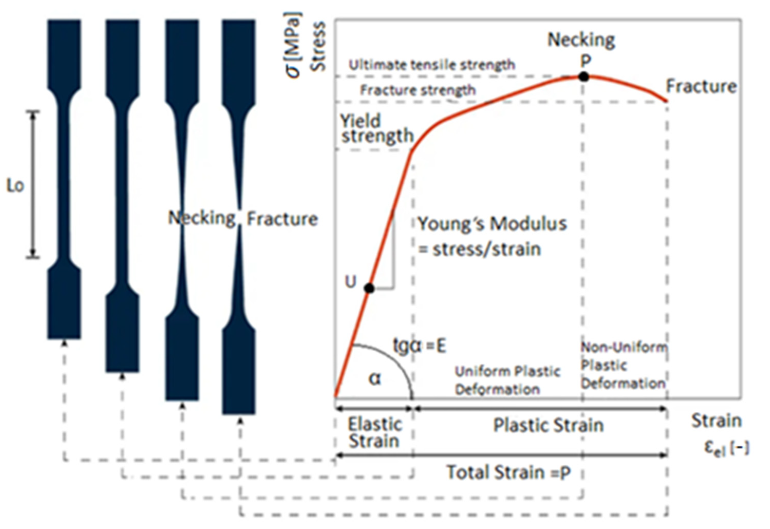
Figure 2 shows the result of testing in form of dependency between strain and stress [5].

Figure 2.
Elongation of the test sample depending on the force applied to the sample [2].
The starting segment of the curve in Figure 2 shows elastic deformation from the reference value to point U. The reversible elastic modulus of material properties is determined by the amount of irreversible elastic deformation that may be induced in individual metal connections before they break. This percentage is typically less than 1%. The next section describes Hooke’s law, which would be phrased as follows:
where represents strain (ratio between total sample elongation and original length), E is sample modulus of elasticity, and σ is mechanical tensile strength.
A tensile sensor directly attached to the testing rod monitors and stores its length. If the expansion of the test section is obtained from the motion of the tearing machine’s cross member, the slant of this section of the tension chart comprises not only elastic behavior of the testing bar but also bending stresses of tearing machine elements—machine frame, dynamometer, and jaws. As a consequence, component E cannot be executed in this case [5].
The deformation remains constant along the section between point U to point P, but still, the linearity is destroyed and there is a deviation from the initial linear trend owing to the onset of plastic deformation accumulation. The stress grows with increasing distortion till it reaches the maximum position of the figure when the specified dependency peaks. The process represented in this area of the figure is strain hardening. Following the consistent narrowing of the detecting section of the testing bar, i.e., the extensometer of the measured area on the test sample, a neck develops at point P, as well as further deformation is associated with a reduction (relaxation) in stress.
After this uneven plastic deformation is finished, i.e., after all viable dislocation sliding mechanisms have been exhausted, the test bar fails. The tensile test is considered successful unless the cracks appear in a specific region of the sample but do not fracture, as well as at the anchoring point [5].
The tensile test is evaluated using UTM using both contact and non-contact methods. Because contact methods are less accurate and more susceptible to shocks and temperature fluctuations, they are not recommended. Non-contact methods for tensile test evaluation are covered next in our research [6].
2. Non-Contact Methods for Tensile Test Evaluation
Contact extensometers are extensively used in material testing to detect axial stresses in test objects with high flexibility, such as metal or hard polymers. Although these touch sensors enable maximum stress monitoring in a variety of applications, they have the disadvantages of careful operator interaction, decreased flexibility, and limited application for the reasons listed below [7].
Their weight and method of attachment might affect the load–strain response of the test specimen, restricting their usage on polymeric, biological products, and composite material. Additionally, sufficient tension should be implemented to avoid the cutting edges or clip-on wires shapes installed on the sample from sliding, which might contribute to catastrophic failures [8].
A physical extensometer can only measure one-directional (often vertical) strain summed over the gauge length. Additionally, physical extensometers intended for room temperature usage cannot be utilized in other environments (high or low temperature).
For universal testing assessment, there are two main types of non-contact measurement methods. Laser extensometry, as well as video extensometry, are two often used systems [9].
2.1. Video Extensometry
A video extensometer (Figure 3) is a measurement system composed of one or more cameras, as well as image processing algorithms.

Figure 3.
Video extensometry.
Camera extensometers based on functionality image-processing machine learning track the geometric properties (e.g., centroids, edges) of various artificial signs (e.g., circular pattern dots, print strips (welded tracks) that can be depicted, glued, attached, or concocted onto the test sample and measuring the surface stains of a sample [10].
Aside from functionality object recognition, intensity-based picture comparison approaches based on the digital image correlation (DIC) can also be used. DIC is a powerful optical method that is commonly used in experimental physics for filled displacement and strain measurements. It is commonly employed as a post-processing technique with enhanced registrations precision but a significant computational cost. Using recent developments in subpixel registration methods, efforts have been made to utilize DIC in real-time movement and tension monitoring [11].
Basic image processing is used in our study, as well as more advanced image processing methods, such as DIC correlation, which will be addressed further in the next chapter [12].
2.2. Laser Extensometry
Material testing system manufacturers have worked hard over the years to produce innovative non-contact material testing strain measuring methods. Laser scanners are one of the alternatives being examined, as they have proven to be particularly useful for several materials, such as plastics, film, rubber, and textiles. Users of tensometers have also wanted more information, flexibility, and variety from their devices. Non-contact technologies, such as laser-based extensometers for traction machines, were among the first to appear. These devices were accurate when measuring significant strains, but they lacked flexibility and were less accurate when measuring very low-level strains [13].
Traditional clip-on or contact extensometers are often used to test materials that could be damaged or affected by laser extensometers. They work by using a laser to illuminate a specimen’s surface and then recording the laser reflections as force is applied. Advanced imaging software with complex algorithms is then used to measure these reflections. Because they may be used with a wide range of materials and tests can be conducted on specimens at increased as well as ambient temperatures, laser-based systems are ideal for samples housed in a thermal cabinet or environmental test chamber [14].
Laser extensometers also offer high accuracy and resolution, as well as a level of safety, which is especially important for assessing specimens that could release a lot of energy if they fail [15].
3. Proposed System of Video Extensometry
Our primary goal was to create a non-contact system for measuring geometrical properties with an accuracy that is sufficient to evaluate the basic parameters of material sample under tensile testing. The measurement accuracy of our system is discussed in the results section and is in accordance with generally applicable standards in commercially used systems, see [5,6,7,8,9,10,11,12,13,14,15]. The key parameter defining the accuracy of distance measurements is resolution of the camera and the accuracy of its calibration.
Another goal was to develop new functionality which enables the prediction of cracking sites, which is an important part of research that contributes to a better and more accurate evaluation of the measured data. The novelty is in the use of a single high-resolution inspection CMOS camera, which reduces costs and, at the same time, facilitates the handling and calibration of the system. In the basic mode, the reflection marks (points) are not placed on the material sample. Our measuring system can measure the required data in real-time without the use of these additional marks. To improve the accuracy of the measurement, it is possible to create different reflective patterns for the tested sample.
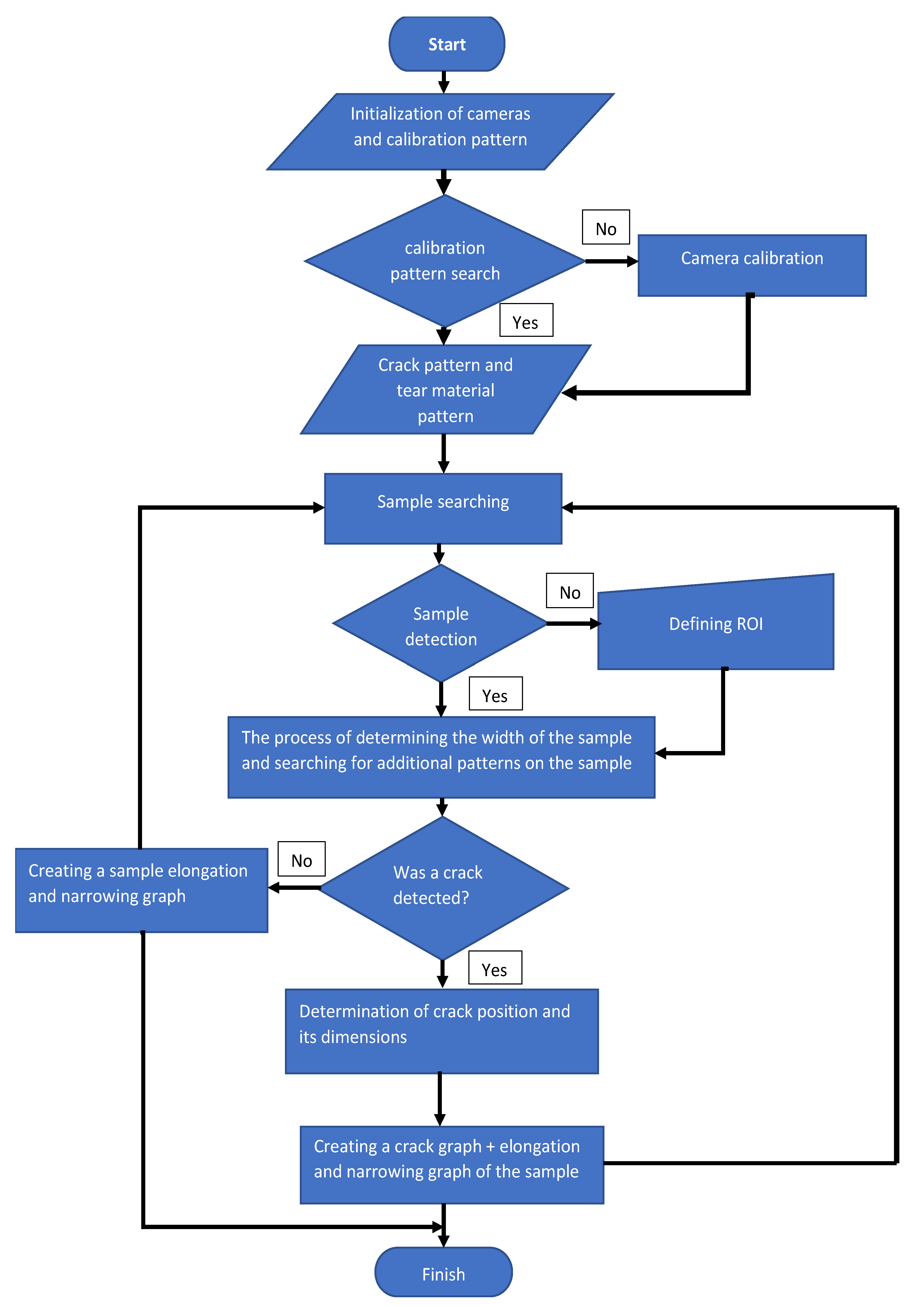
Based on the declared conditions, the basic algorithm flowchart is shown in Figure 4. Single image processing and analysis algorithms will be discussed in another section of this article.
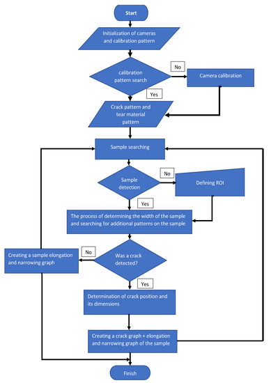
Figure 4.
Flowchart of our algorithm.
The first step in the measurement algorithm is camera calibration when the distortion of lens is corrected. It is necessary to know the distance between the camera and the measured sample at the start of the measurement and use the appropriate calibration pattern.
Pattern matching is a image segmentation technique based on normalized cross-correlation between the inspected image and a given image template. In the proposed algorithm, pattern matching serves for localization of the material sample in the image and later for crack occurrence detection. If the material sample is found by pattern matching, the next image processing is conducted in a region of interest (ROI) instead of the entire image (processing is then faster). If the algorithm fails to locate the measurement sample, a ROI can be manually created [16].
After the material sample is localized in the image, the image algorithm focuses on determining the sample’s edges using selected edge detectors (e.g., Canny edge detector). If any additional marks and patterns are present, such as various lines or points added to the sample by color, engraving, or welding methods, their detection, along with detection of sample borders, allow to determine the width and height of the sample more precisely at any given measurement point.
When looking for additional patterns on the measuring sample, the algorithm also looks for cracks and predicts where cracks are most likely to appear soon, before tearing the sample. The algorithm creates an ROI in the place of a future crack, or in the place of an already created crack, after predicting the places where a crack is most likely to occur. The algorithm then determines the parameters of the crack (if one has already occurred), such as its height, width, and crack propagation direction [16].
Finally, the results of the entire tensile test are plotted as changes in the length and width of the sample over time, as well as determining the time of crack formation on the sample and graphically showing its propagation throughout the measurement.
3.1. Camera Callibration
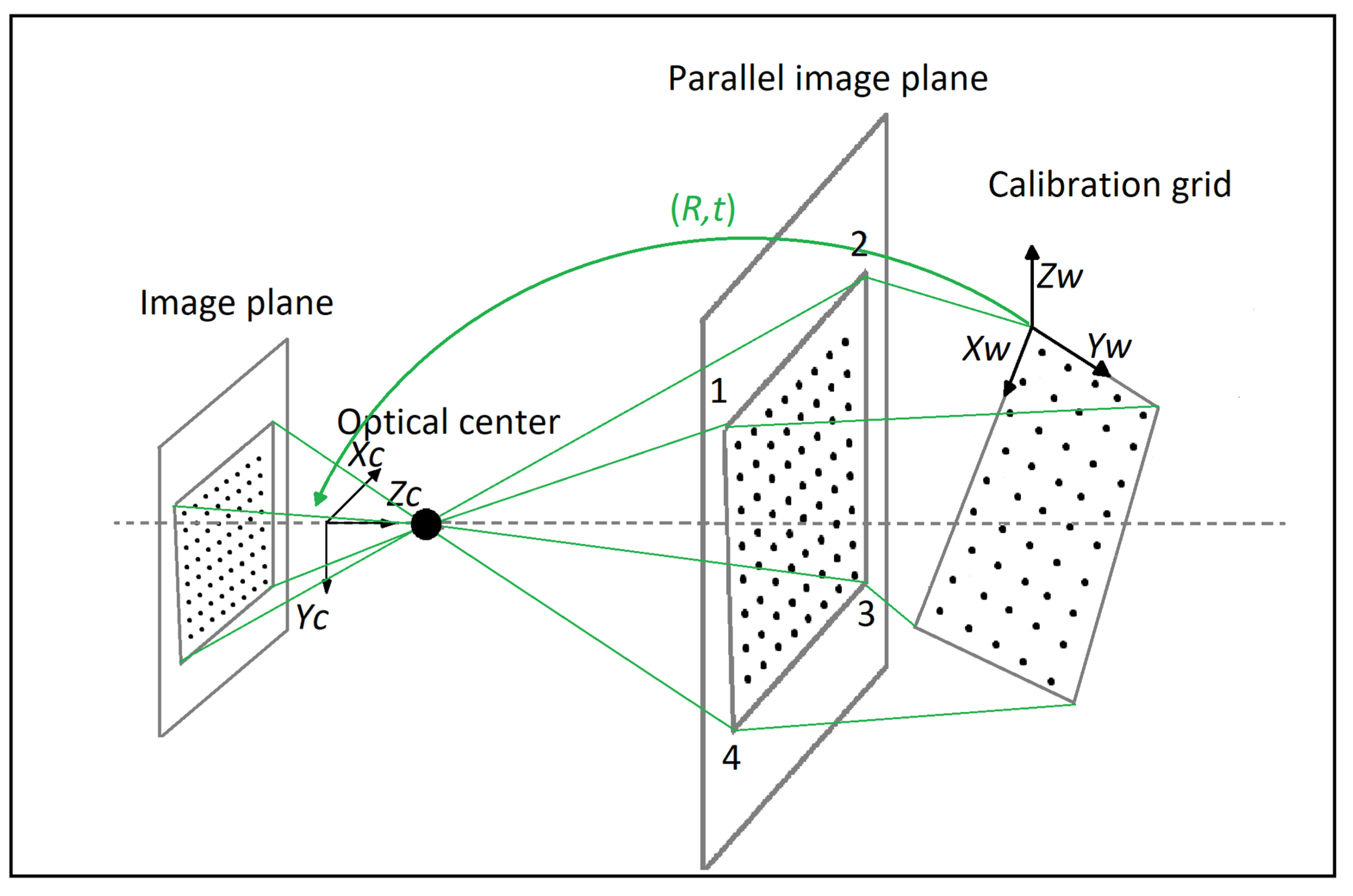
It is necessary to understand which factors are responsible for the image and how to use these factors to map coordinates from the real world to the image coordinates to properly calibrate the camera [16]. Figure 5 represents projective mapping.
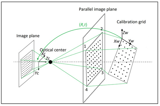
Figure 5.
Projective mapping.
The calibration grid is represented by a real-world coordinate frame (xw, yw, zw). The image orientation is (xc, yc, zc), with the z-direction connected with the image plane and the x and y axes oriented with the horizontal and vertical axes of the image plane [16].
An intermediary plane parallel to the picture plane depicts the form of the calibrating object in an image.
An image coordinate axis is shifted away from a real-world coordinate’s axis using the following formula:
where Pw marks the point in the real-world coordinate frame, Pc stands for the homogeneous point in the camera coordinate system, T is the real-world position axis’ origin excluding the camera reference axis’ origin, and R is the rotation vector between the real-world point axis and the camera point axis [17].
Mechanical projecting, also called homography, is a geometrical transfer of coordinates through one plane to another. The transfer of 3D information in the current world to pixel location in a picture in calibration is described by homography.
The main point P (xw, yw, zw) is transformed into the picture point p through a physiological predictive conversion (xw, yw).
An illustration of homography is as follows:
The picture planes projections in image coordinates [xc yc 1]T, which are 2D object coordinates, is denoted by p. P is a [xw yw zw 1]T real-world point represented in 3D real-world dimensions. The symbol s represents scaling factor, while the letter H indicates homography.
When utilizing validation software, homography (H) is a 3 × 3 matrix which is the sum of two matrices: a video matrix (M) and a homography matrix (W) [17].
The accompanying video matrix (M) is presented in the form of camera properties, such as central focus length, primary point location, pixel sizes, and pixel distortion angle:
where:
The focal length is represented by the symbol F in mm. The horizontal length of a pixel in an image sensor is equivalent to sx in pixels per millimeter. The vertical dimension of a pixel in the imaging system is measured in pixels per millimeter. The horizontal distance between the imager and the visual axis is measured in millimeters by cx and the most frequent number is 0. cy is the imager’s vertically offset from the optical system in millimeters and is also the pixel distortion angle of signal with respect to x.
A camera’s field of view (F) and pixel sizes (sx, sy) are not immediately calculable. The vision system (fx, fy) can only estimate derivatives focal distance and pixel size combinations [17].
A homography matrix is made up of the transformation matrix and translations vector that relate a location in the real-world plane to a position in the picture plane (W). The following is the mechanical projection modulation index:
R is the spin matrix, while t denotes the translation vector. As seen below, the rotation matrix ® may be expressed as three independent 3 × 1 matrices:
As a result, the previous homography (3) could be written as follows:
We may extend that Z equals 0 since validation is performed using a flat calibration object.
It is also critical to keep optics and sensor distortion to a minimum in calibration. There are two sorts of distortions that are frequently seen. Lens features can produce radial distortion, whereas a misalignment of the optics and camera system can create tangential deformation.
The polynomial deformation model is used to eliminate tangential and radial deformation. The polynomial deformation model uses one or much more contribution parameters to model deformation (K). The accompanying deformation model represents radial deformation:
The polynomial deformation concept employs two variables, P1 and P2, to quantify tangential deformation. The accompanying deformation model represents tangential deformation:
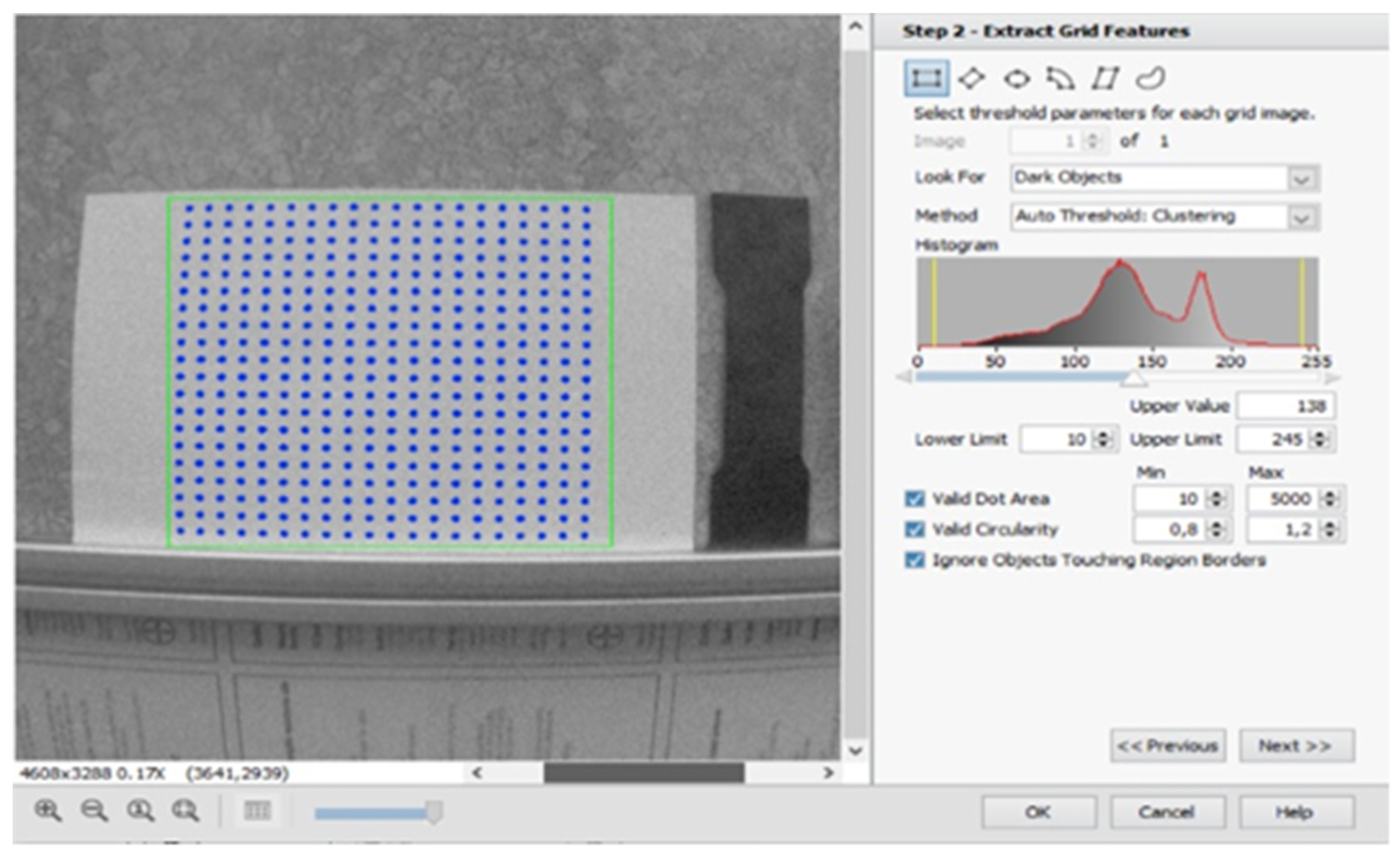
To calibrate the cameras, we used NI’s Vision Assistant software. Calibration of the camera is done in several steps. The first step was to create a calibration grid, as shown in Figure 6. Following that, basic image processing methods such as thresholding or edge detection are used to determine the position of each point of the calibration grid [17].
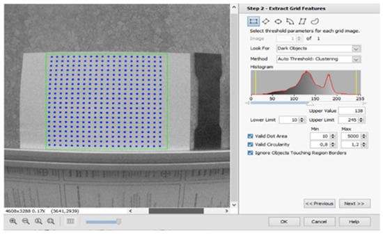
Figure 6.
Calibration grid captured by camera.
We can convert each distance in pixels to the actual distance in millimeters because each point on the grid is 10 mm apart. We used a polynomial distortion model with three coefficients, K1, K2, and K3, to reduce tangential and radial distortion.
A map of distorted points is shown in Figure 7, with white dots representing error pixels. We achieved high accuracy in evaluating the dimensions of the measured object using this calibration method, with the highest error rate being 0.006 mm.
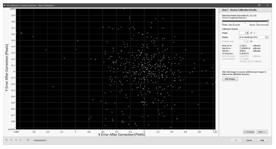
Figure 7.
Map of distorted points in calibration process.
3.2. Pattern Matching
Pattern matching is an algorithm which belongs to the group of template matching algorithms. It is used in two critical phases of our algorithm: to locate a material sample and to find cracks in the sample.
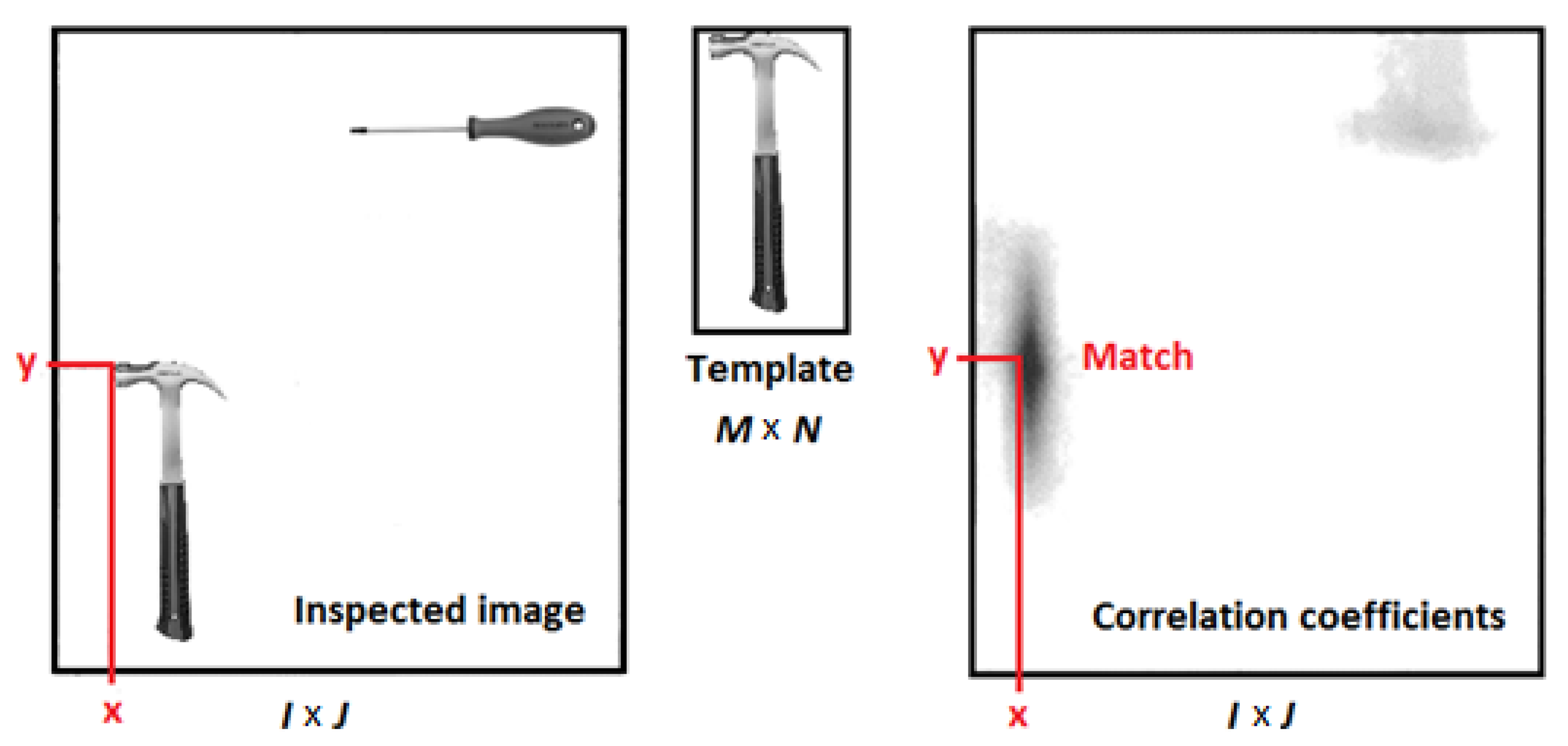
Pattern matching is a relatively simple method for localization of selected (template) patterns in an inspected image. If the searching template is selected, the process of normalized cross-correlation between the template and image is provided. The correlation score ranges between −1 and +1. Even though pattern matching is generalized for color images, greater efficiency can be provided by using the intensity layer of an image (monochromatic, grayscale). Then, the cross-correlation algorithm looks for locations with the greatest cross-correlation score in the inspected image to find matches (Figure 8) where I × J is dimension of original image and M × N is dimension of template image [18].
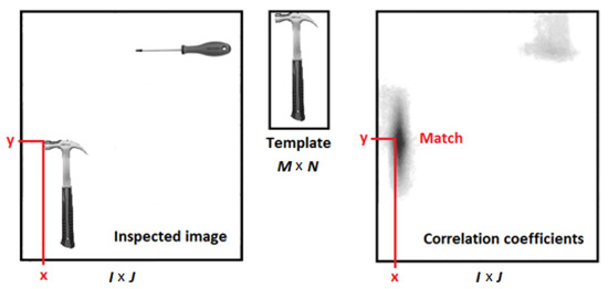
Figure 8.
Cross-correlation between image and pattern.
Normalized cross-correlation is now the most frequent approach for identifying a pattern in an image. Because the exact principle is dependent on a sequence of multiplication operations, the correlation process can be included. With innovations like MMX, that minimize total process time, multiple equations are achievable. To allow a faster validation process, we lower the length of the picture and confine the region of interest (ROI) where the matching happens. Pyramidal comparisons and object recognition are two ways for speeding up the validation process.
Standardized cross-correlation is a useful approach for discovering patterns in images that have not been scaled or rotated. Cross-correlation may identify trends with the same length with a rotation of 5° to 10°. Extending correlation to find patterns that are not influenced by scale or spin is tricky. Continuing the scaling or resizing step and then conducting the correlation operation is required for scale-invariant finding. As a result, the search algorithm will need a substantial amount of computing. Normalizing for rotation is significantly more challenging. We just spin the pattern and perform the correlation process if indeed the image offers a clue about rotation. If the type of rotation is uncertain, the template must be rotated indefinitely to discover the best fit. By using a particles strategy, pyramidal fitting, or feature detection, we can reduce the amount of processing time considerably and reach reasonable search speeds for spinning patterns [18].
In pyramidal fitting, both the picture and the pattern are sampled to decrease spatial information using Gaussian pyramids. This approach samples almost every pixel for each successive pyramid step, allowing the picture and pattern to be shrunk to one of their initial sizes.
The system estimates the greatest pyramid degree that may be utilized for a part of an opening during the process of learning, and then stores the data needed to represent the pattern and its rotated variants at all processing levels. The program aims to establish an appropriate pyramid standard based on the set that will deliver the fastest and most efficient match. Grey values (based on image brightness) and gradients (based on chosen edge information) are two forms of data that may be employed [18].
The comparison stage uses a coarse-to-fine strategy, with our search starting at the smallest resolution possible (the highest pyramid level). Since the dimensions of the research image and pattern have been considerably reduced at this resolution, we can conduct a comprehensive correlation-based search. The subsampling approach, on the other hand, results in a significant loss of detail, and the match sites are not always exact. This challenge is overcome by retaining a list of potential candidate match sources with the highest ratings, rather than deciding the precise number of matches to seek for. We then repeat through the lowest layers of the pyramid, improving our selection as we go by recalibrating correlation values at each stage. By confining all future searches to a few confined zones around the greatest match, this technique achieves a significant performance boost [19].
When searching for rotated matches, even at the smallest resolutions, doing an exhaustive search for all conceivable spins (from zero to the field of view) is prohibitively costly. As a result, we begin by determining the best places at a coarse angle. The optimum places are then refined among these coarse sites using a finer angular step size. Then, in the same way, as previously, we tweak the match position and angle over the lowest pyramid levels [19].
For more accuracy, we choose to subject the refined match candidates to one final round of refinement in both pyramidals and low-discrepancy sampling-based pattern matching to find sub-pixel accurate positions and sub-degree precise angles. This stage uses interpolation techniques to obtain a very accurate match position and angle by relying on carefully collected edge and pixel information from the template [20].
Both pattern matching approaches compute a final and correct score using most of the significant information included in the template once the refined locations are achieved [20].
3.3. Labview Application
The whole algorithm for determining the basic parameters of the samples and for detecting and determining the propagation of cracks was created in the LabVIEW environment.
The front panel of the application is shown in Figure 9.
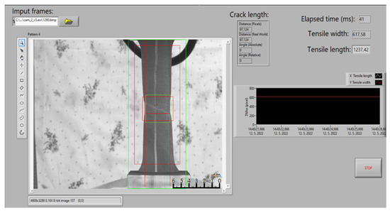
Figure 9.
Front panel of the application in LabVIEW environment.
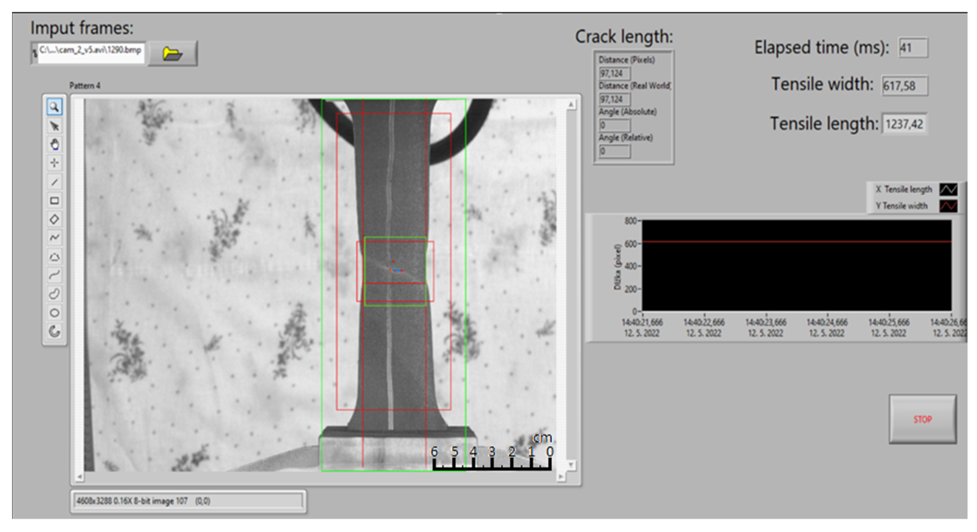
The basic settings for pattern search and pattern parameter determination are located on the left side of the panel. The output image from the camera, as well as the detection of the sample and its contours, are displayed on the right side of the front panel, as shown in Figure 10.
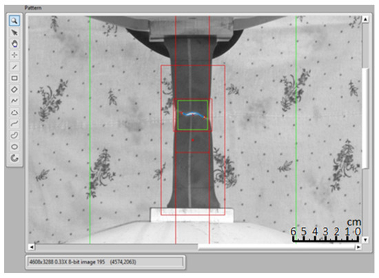
Figure 10.
Output image form the camera.
3.4. Hardware
One of the most important roles in designing a system for video extensometry is selecting the appropriate hardware; without it, this work would be difficult to complete. Because the camera’s properties have such a strong impact on the accuracy of the overall measurement, choosing the right camera for video extensometry is critical.
The high-resolution camera captures fine details of the sample being tested using the Basler ace acA4600-10uc camera with 14 MPix resolution. This camera has spatial resolution of 4608 × 3288 pixels and a pixel size of 1.4 × 1.4 µm, with a frame rate of 10 frames per second. The camera’s tiny size (41 × 29 × 29 mm) makes it portable, as does the flexibility to modify the exposure duration. This camera is intended for use in commercial, medical, and transportation settings [21].
4. Experimental Measurement
The measurement itself consists of two steps. In the first step, calibration and set up of the camera must be completed (including setting the proper exposure time, frame rate, etc.), which is described in paragraph III (A. Calibration).
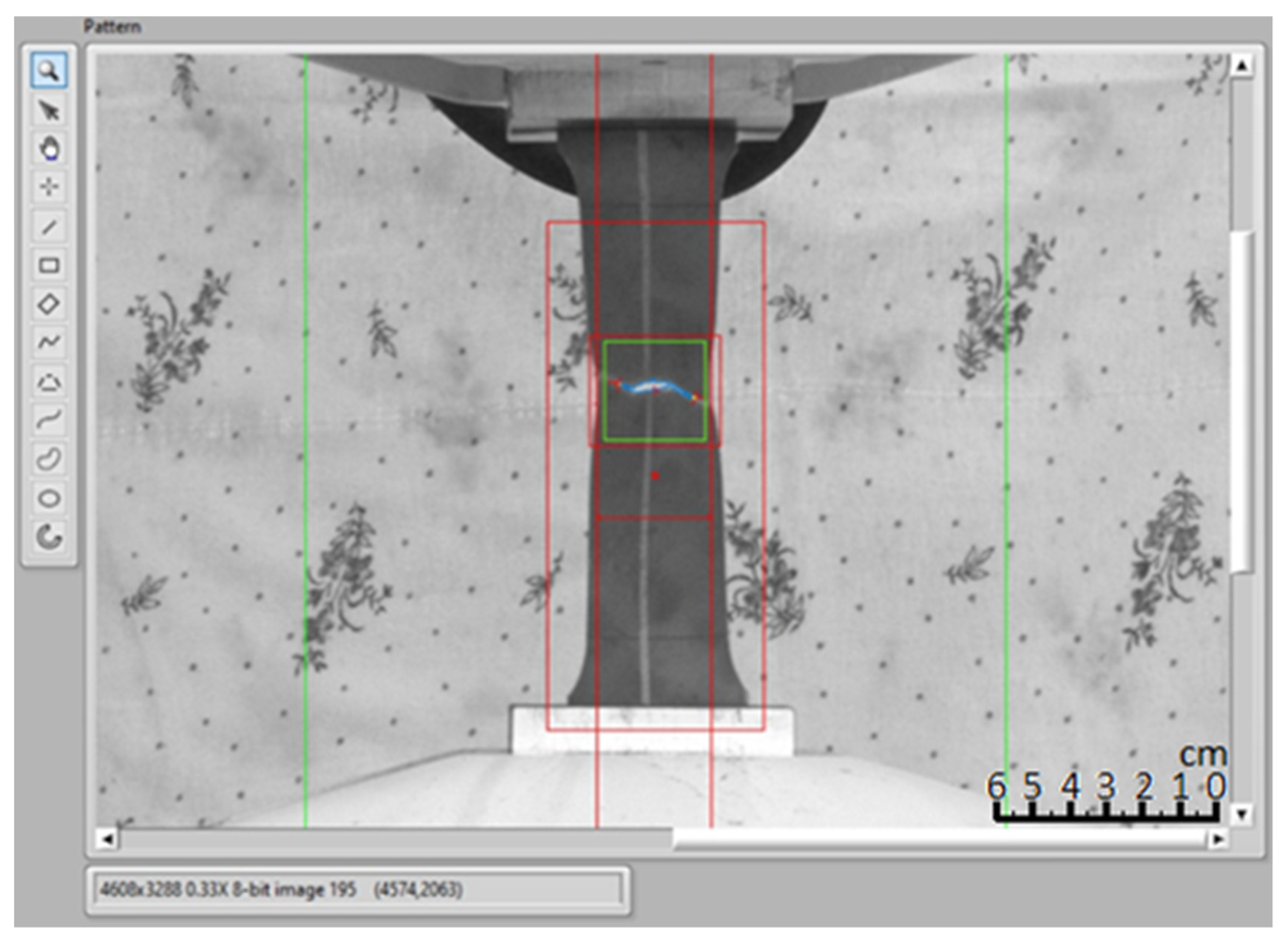
After successful calibration, we proceeded to the measurement itself by first attaching the test sample to the UTM jaws. As can be seen in previous figures, we used non-homogenous background of tested material sample. The background is covered by texture but searching for the material sample were not affected by this fact.
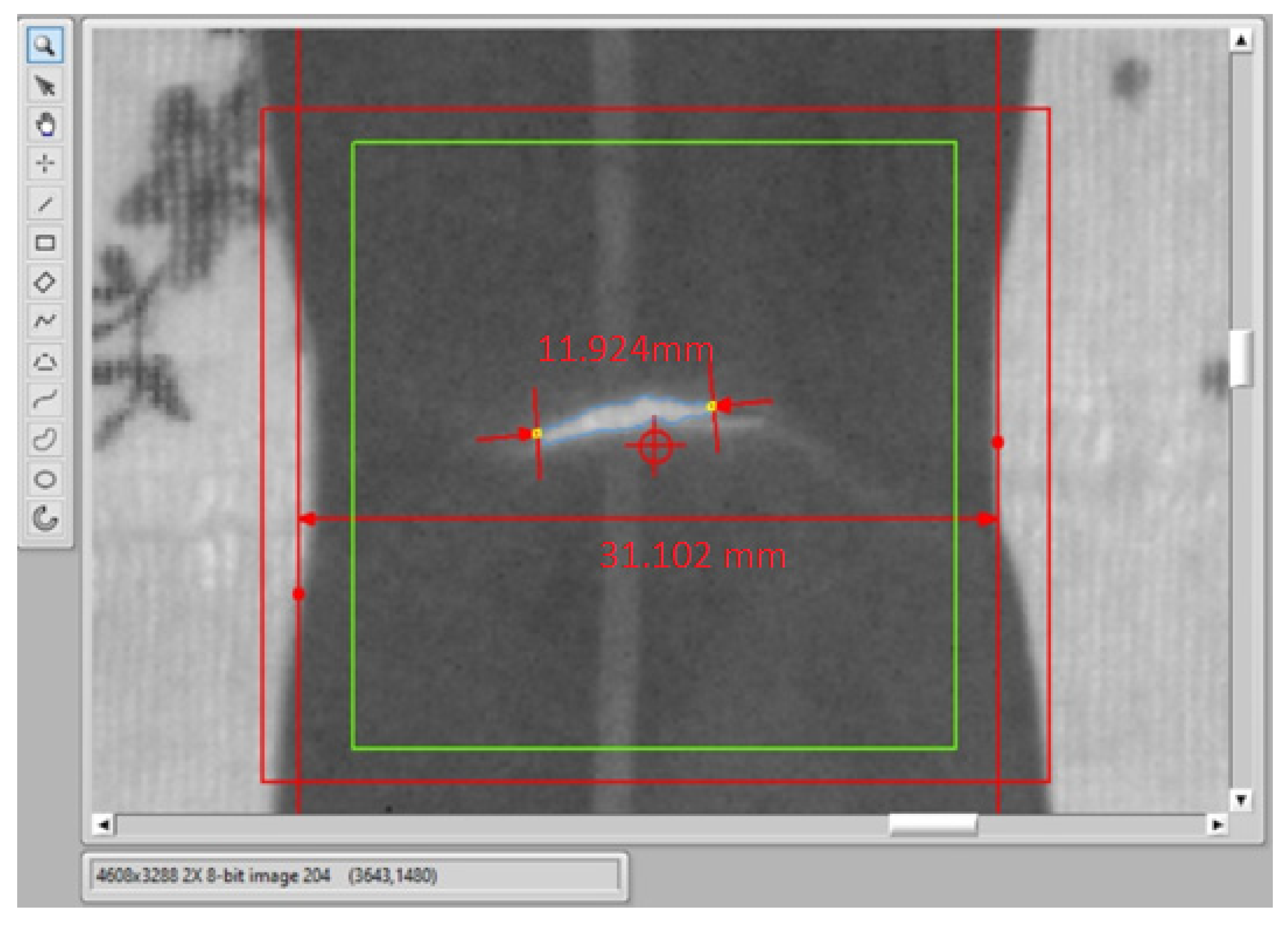
Figure 11 illustrates detecting the crack after its occurrence in the image. The parameters are calculated, such as crack length and width, for each image taken, allowing us to obtain information about the crack propagation during the measurement. After the sample ruptures, the measurement ends.
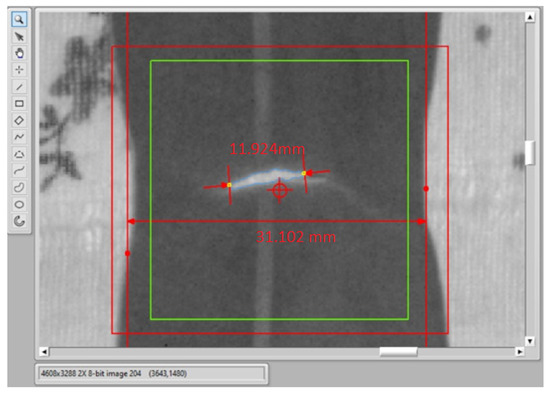
Figure 11.
Detail of the detected crack and measurement of its properties.
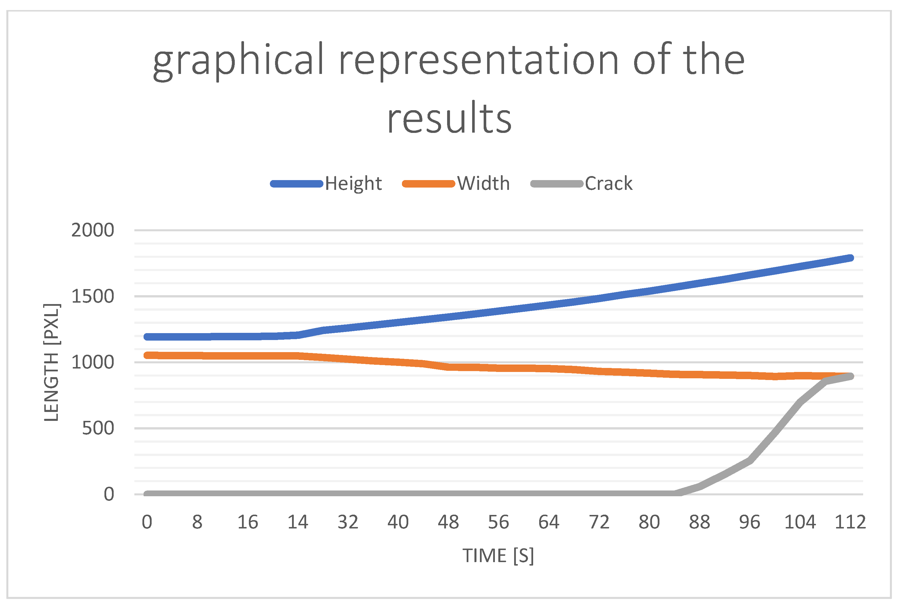
There are two ways to evaluate the measurement images. The measurement can be performed in two modes. The first mode is offline, when the entire tensile testing is captured in video sequence and then frame-per-frame processed with image algorithms. The second mode is online (“real-time”), when the image frames are processed instantly. We understand the real time in following manner: the image frame is processed in the time before another frame comes from the camera. Having the information from Table 1, we can see that the time for pattern matching procedure (which takes the most of operational time) takes approximately 50 ms. Since the camera Basler runs a maximum of 10 fps, the computational time for image algorithms is sufficient. The graphical output of measurement plotting the actual length and width of the sample in time can be seen in Figure 12.

Table 1.
Comparison of results.
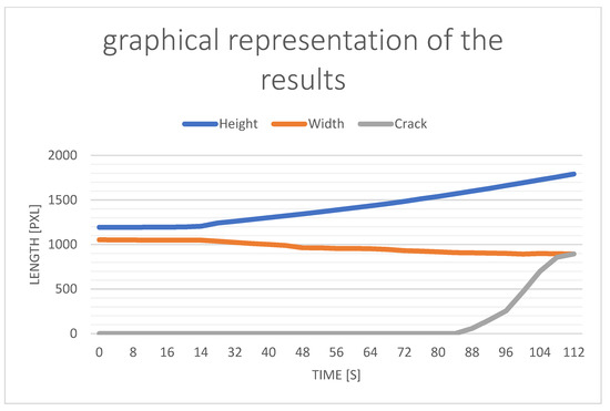
Figure 12.
Graphical representation of the results.
5. Discussion
To discuss the results of proposed video-extensometric system we can analyze the following key parameters: how successfully were the image regions (sample localization and crack occurrence) detected by pattern matching technique; accuracy of setting the geometrical distances of material sample; and computational time of proposed method with another commercially used techniques. Commercially-used techniques were adapted to LabVIEW environment based on relevant bibliography research. Only video-extensometric methods operating in visible light range were compared, since laser methods are based on different principle.
All techniques were simulated on a single computing device, and these methods used data from the same camera, even when comparing the estimation speed and efficiency of individual methods. The calculations were carried out on a computer with an AMD RYZEN 5 4600H processor, 8 GB DDR4 RAM, and an NVIDIA GeForce RTX 2060 graphics card (Lenovo Legion 5, Beijing, China). As a result, the factor of computing device performance, as well as the factor of significant resolution of camera images, can be ignored when implementing individual image processing methods. The average calculation times and accuracy of the image processing methods are shown in Table 1.
From experimental results, we can see that all mentioned methods are suitable for real time mode of measurements, because computational time does not exceed 100 ms (for 10 fps maximal rate of used camera). Even though the proposed methods need the biggest computational time, high-resolution chip of camera enables the localization and geometric distances measurements up to 0.006 cm accuracy.
Pattern matching detection success rate was measured on dataset of approximately 10,000 video frames. The sample position, as well as the crack position, was evaluated in Table 2.
Table 2.
Pattern matching detection success rate.
6. Conclusions
Based on the experimental results, we can conclude that proposed video-extensometry system is a non-contact system with high potential to do the tensile testing fully automated. Non-contact approach does not need any mechanical sensor affecting the sample under test. Comparing with existing commercial systems based on video capture, our system also does not need reflections marks and patterns in basic mode (just for improving the accuracy).
Based on the cited references [22,23,24,25,26,27,28], we can pronounce those methods based on DIC correlation as being the gold standard in optical methods of material tensile testing and have significant advantages. Our proposed method can be the alternative way to automatize tensile tests using image functions which differ from classical correlation and achieve comparable results.
DIC correlation requires, at each step, the calculation of the position of the patterns that are added to the sample (contrast injection on the sample). This process is computationally intensive and, therefore, burdens the computing device. It is also necessary to use specialized cameras with high resolution and several lighting devices due to the stability of the entire measurement system. To reduce the demands on computing equipment, modifications of DIC correlation have been developed, such as the method of Bin Chen et al. [12], which calculate only certain areas of the sample, which speeds up the measurement itself, but on the other hand, loses information about the remaining parts of the sample. Our method does not require any artificial intervention in the sample and performs sample searches only in the initial step and is, therefore, less demanding on computing equipment. Many UTMs consist of a protective glass that is in front of the test sample. If an additional light source is used in such a case, unwanted light reflections from the protective glass will occur, which reduces the accuracy of the measurement itself. The method proposed by us does not need additional light sources and was also tested in experimental measurements using protective glass with very accurate results.
Another advantage of our system is in the usage of a single high-resolution inspection camera. On the other hand, the camera must be properly calibrated to obtain accurate measurement. Our method also does not require the exact location of the camera and the test object. The only procedure which is needed to do before the measurement is camera recalibration.
It is also worth noting that DIC correlation algorithms with optical flow are much more susceptible to lighting changes, which can decrease their accuracy and this method is extremely accurate locally (in a selected area).
Last, but not least, the advantage of the proposed system is the detection or prediction of the location of crack occurrence. The time of crack origin and its dimension or orientation are part of the measurement report for a given tensile test.
Just as the advantages of our measurement system were highlighted, it is also necessary to point out the disadvantages (limitations) of the proposed system. Since the measuring system was tested only on metal and rubber samples, it cannot be said with certainty that its accuracy will be the same during the testing of other materials. Another disadvantage of the measurement system is that it is important that the camera is placed far enough from the UTM due to vibrations that could worsen the accuracy of the evaluation of the measured data.
Author Contributions
J.B.: Primary writing, structuring, and formatting; L.H.: secondary writing and primary review; D.K.: generative design case-study, visuals, and secondary writing. All authors have read and agreed to the published version of the manuscript.
Funding
This research was supported by the following grants: APVV 15-0462—Research on sophisticated methods for analyzing the dynamic properties of respiratory epithelium’s microscopic elements; APVV 17-0218—Investigation of biological tissues’ interactions with high-frequency electromagnetic fields and their use in the creation of innovative techniques in the design of electrosurgical equipment. APVV 20-0500—Methodologies for improving the quality and longevity of hybrid power semi-conductor modules are being researched.
Institutional Review Board Statement
Not applicable.
Informed Consent Statement
Not applicable.
Data Availability Statement
Not applicable.
Conflicts of Interest
The authors declare no conflict of interest.
References
- Saba, N.; Jawaid, M.; Sultan, M.T.H. An Overview of Mechanical and Physical Testing of Composite Materials; Woodhead Publishing: Sawston, UK, 2019; ISBN 978-0-08-102292-4. [Google Scholar]
- Kašuba, M. Analysis of the Miniature Test Specimen Results with Variable Geometries. Available online: https://www.vutbr.cz/www_base/zav_prace_soubor_verejne.php?file_id=15103 (accessed on 30 May 2021).
- MatNet Slovakia. Static Tensile Test. Available online: http://www.matnet.sav.sk/index.php?ID=526 (accessed on 30 May 2022).
- Zheng, P.; Chen, R.; Liu, H.; Chen, J.; Zhang, Z.; Liu, X.; Shen, Y. On the standards and practices for miniaturized tensile test—A review. Fusion Eng. Des. 2020, 161, 112006. [Google Scholar] [CrossRef]
- Tran, K.Q.; Satomi, T.; Takahashi, H. Tensile behaviors of natural fiber and cement reinforced soil subjected to direct tensile test. J. Build. Eng. 2019, 24, 100748. [Google Scholar] [CrossRef]
- Ma, Q.; Rejab, M.R.M.; Qayyum, H.; Merzuki, M.N.M.; Darus, M.A.H. Experimental investigation of the tensile test using digital image correlation (DIC) method. Mater. Today Proc. 2020, 27, 757–763. [Google Scholar] [CrossRef]
- Vukelic, G.; Vizentin, G.; Ivosevic, S. Tensile strength behaviour of steel plates with corrosion-induced geometrical deteriorations. Ships Offshore Struct. 2021, 54, 154–162. [Google Scholar] [CrossRef]
- Tao, G.; Xia, Z. A non-contact real-time strain measurement and control system for multiaxial cyclic/fatigue tests of polymer materials by digital image correlation method. Polym. Test. 2005, 24, 844–855. [Google Scholar] [CrossRef]
- Pan, B.; Tian, L. Advanced video extensometer for non-contact, real-time, high-accuracy strain measurement. Opt. Express 2016, 24, 19082–19093. [Google Scholar] [CrossRef] [PubMed]
- Dong, B.; Tian, L.; Pan, B. Tensile testing of carbon fiber multifilament using an advanced video extensometer assisted by dual-reflector imaging. Measurement 2019, 138, 325–331. [Google Scholar] [CrossRef]
- Shao, X.; Eisa, M.M.; Chen, Z.; Dong, S.; He, X. Self-calibration single-lens 3D video extensometer for high-accuracy and real-time strain measurement. Opt. Express 2016, 24, 30124–30138. [Google Scholar] [CrossRef] [PubMed]
- Chen, B.; Chen, W.; Pan, B. High-accuracy video extensometer based on a simple dual field-of-view telecentric imaging system. Measurement 2020, 166, 108209. [Google Scholar] [CrossRef]
- Dong, B.; Li, C.; Pan, B. Ultrasensitive video extensometer using single-camera dual field-of-view telecentric imaging system. Opt. Lett. 2019, 44, 4499–4502. [Google Scholar] [CrossRef] [PubMed]
- Zhang, X.; Bech, J.; Hansen, N. Low temperature annealing of cold-drawn pearlitic steel wire. Conf. Ser. Mater. Sci. Eng. 2015, 89, 012058. [Google Scholar] [CrossRef] [Green Version]
- Pan, B. Digital image correlation for surface deformation measurement: Historical developments, recent advances and future goals. Meas. Sci. Technol. 2018, 29, 082001. [Google Scholar] [CrossRef]
- Bulava, J.; Hargas, L.; Koniar, D.; Stefunova, S. Determination of material parameters using video extensometry during tensile testing. In Proceedings of the 2021 International Conference on Electrical Drives & Power Electronics (EDPE), Dubrovnik, Croatia, 22–24 September 2021. [Google Scholar]
- National Instruments Corp. Determining the Pose of an Object. 2022. Available online: https://zone.ni.com/reference/en-XX/help/372916M-01/nivisionconcepts/spatial_calibration_indepth/ (accessed on 30 May 2021).
- Sinkovics, N. Pattern matching in qualitative analysis. In The SAGE Handbook of Qualitative Business and Management Research Methods: Methods and Challenges; Cassell, C., Cunliffe, A.L., Grandy, G., Eds.; Sage Publications: Thousand Oaks, CA, USA, 2018; pp. 468–484. ISBN 9781526429278. [Google Scholar]
- Hak, T.; Dul, J. Pattern Matching. ERIM Report Series Reference. No. ERS-2009-034-ORG. 2009. Available online: https://ssrn.com/abstract=1433934 (accessed on 30 May 2022).
- Davis, J.R. Tensile Testing; ASM International: Materials Park, OH, USA, 2004; ISBN 9781615030958 1615030956. [Google Scholar]
- Edmund Optics Inc. Basler Ace acA4600-10uc Color USB 3.0 Camera. Available online: https://www.edmundoptics.com/p/basler-ace-aca4600-10uc-color-usb30-camera/32436/ (accessed on 30 May 2022).
- Tao, Q.B.; Benabou, L.; Tran, N.H.; Luu, D.B. A Digital Image Correlation setup for the analysis of lead-free solder alloys. In Proceedings of the International Conference on System Science and Engineering (ICSSE), Ho Chi Minh City, Vietnam, 21–23 July 2017; pp. 404–407. [Google Scholar] [CrossRef]
- Pelegrin, J.; Bailey, W.O.S.; Crump, D.A. Application of DIC to Extract Full Field Thermo-Mechanical Data from an HTS Coil. IEEE Trans. Appl. Supercond. 2018, 28, 1–5, Art no. 4604305. [Google Scholar] [CrossRef]
- Wang, L. Super-robust digital image correlation based on learning template. Opt. Lasers Eng. 2022, 158, 107164. [Google Scholar] [CrossRef]
- Park, J.; Yoon, S.; Kwon, T.-H.; Park, K. Assessment of speckle-pattern quality in digital image correlation based on gray intensity and speckle morphology. Opt. Lasers Eng. 2017, 91, 62–72. [Google Scholar] [CrossRef]
- Su, Y.; Zhang, Q. A free and open-source software for generation and assessment of digital speckle pattern. Opt. Lasers Eng. 2022, 148, 106766. [Google Scholar] [CrossRef]
- Baldi, A. Robust Algorithms for Digital Image Correlation in the Presence of Displacement Discontinuities. Opt. Lasers Eng. 2020, 133, 106113. [Google Scholar] [CrossRef]
- Ghulam Mubashar, H. Digital Image Correlation for discontinuous displacement measurement using subset segmentation. Opt. Lasers Eng. 2019, 115, 208–216. [Google Scholar] [CrossRef]

Publisher’s Note: MDPI stays neutral with regard to jurisdictional claims in published maps and institutional affiliations. |
© 2022 by the authors. Licensee MDPI, Basel, Switzerland. This article is an open access article distributed under the terms and conditions of the Creative Commons Attribution (CC BY) license (https://creativecommons.org/licenses/by/4.0/).