
Rapid Detection of Cardiac Pathologies by Neural Networks Using ECG Signals (1D) and sECG Images (3D)

 ,
,  ,
,
Abstract
:1. Introduction
2. Materials and Methods
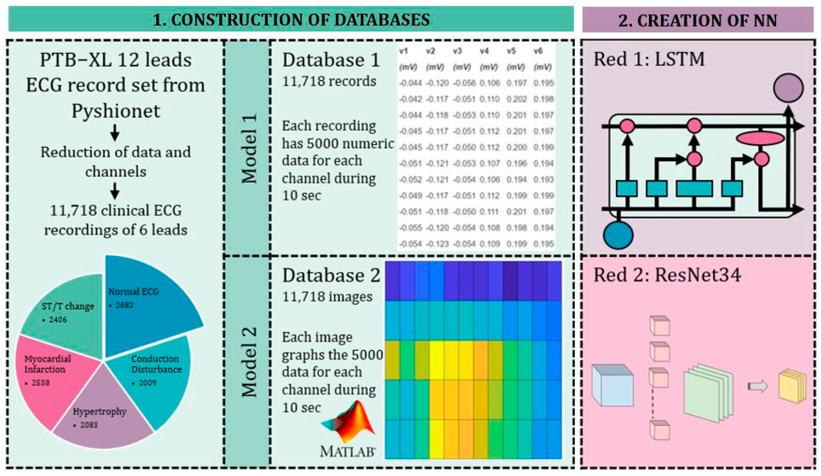
2.1. Databases
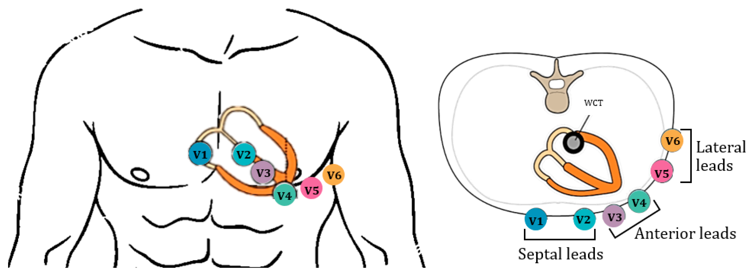
2.1.1. Database 1: Process of ECG Signals
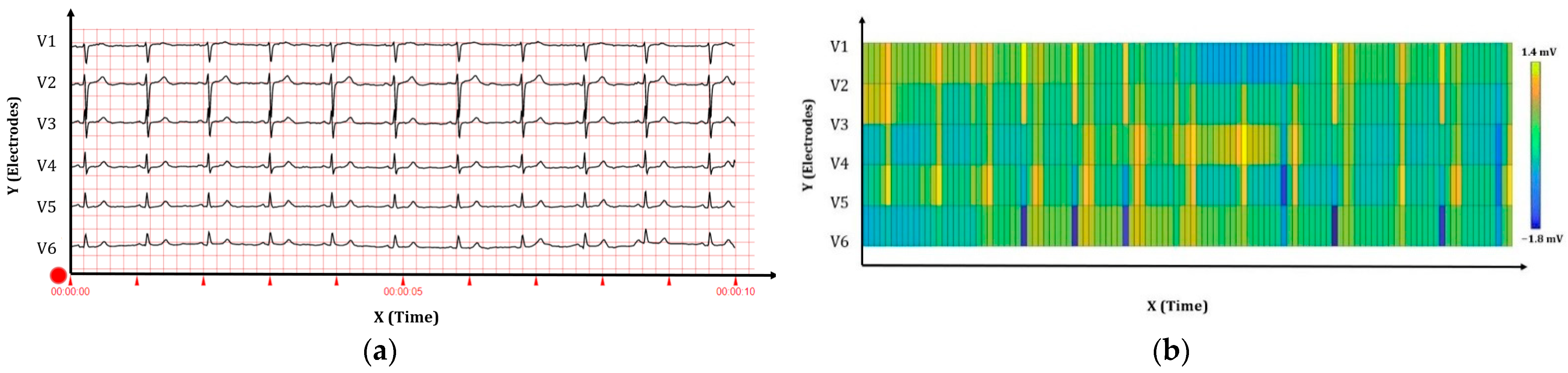
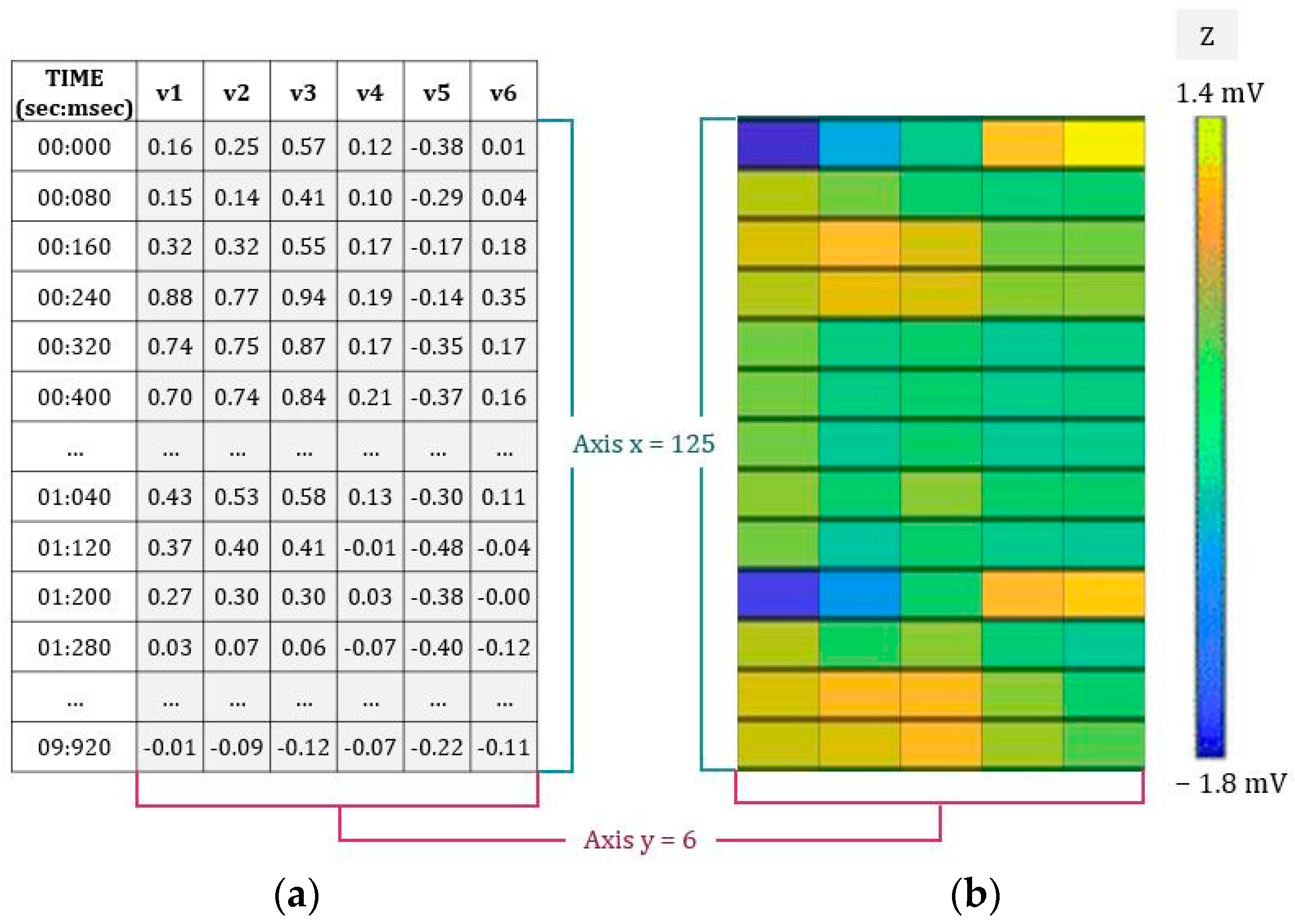
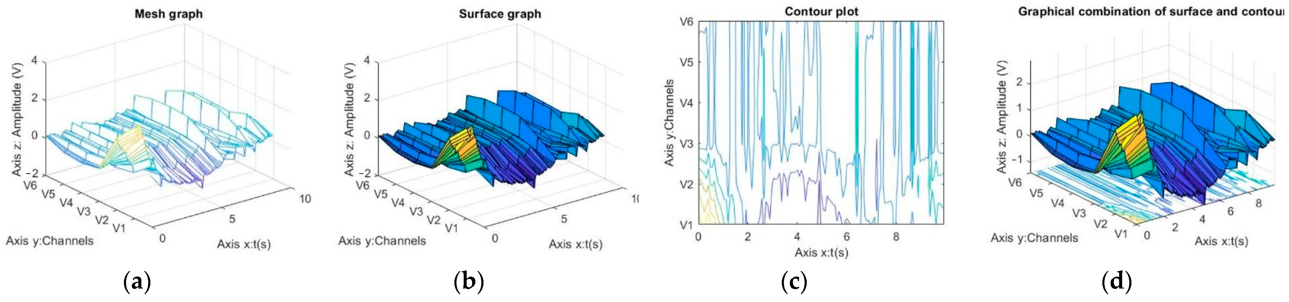
2.1.2. Database 2: Construction of the sECG Images
2.2. Neural Networks
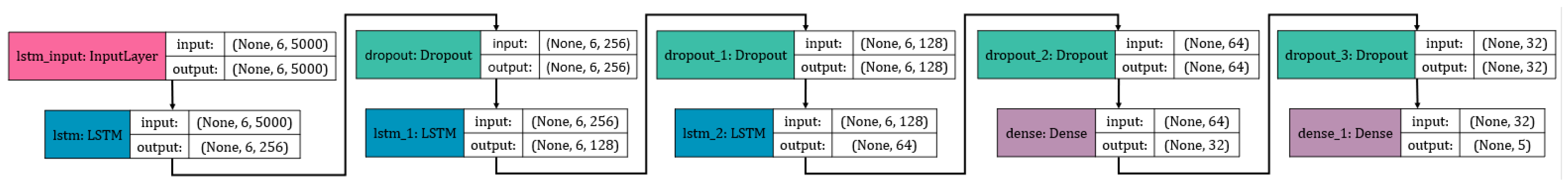
2.2.1. Computational Analysis: LSTM NN
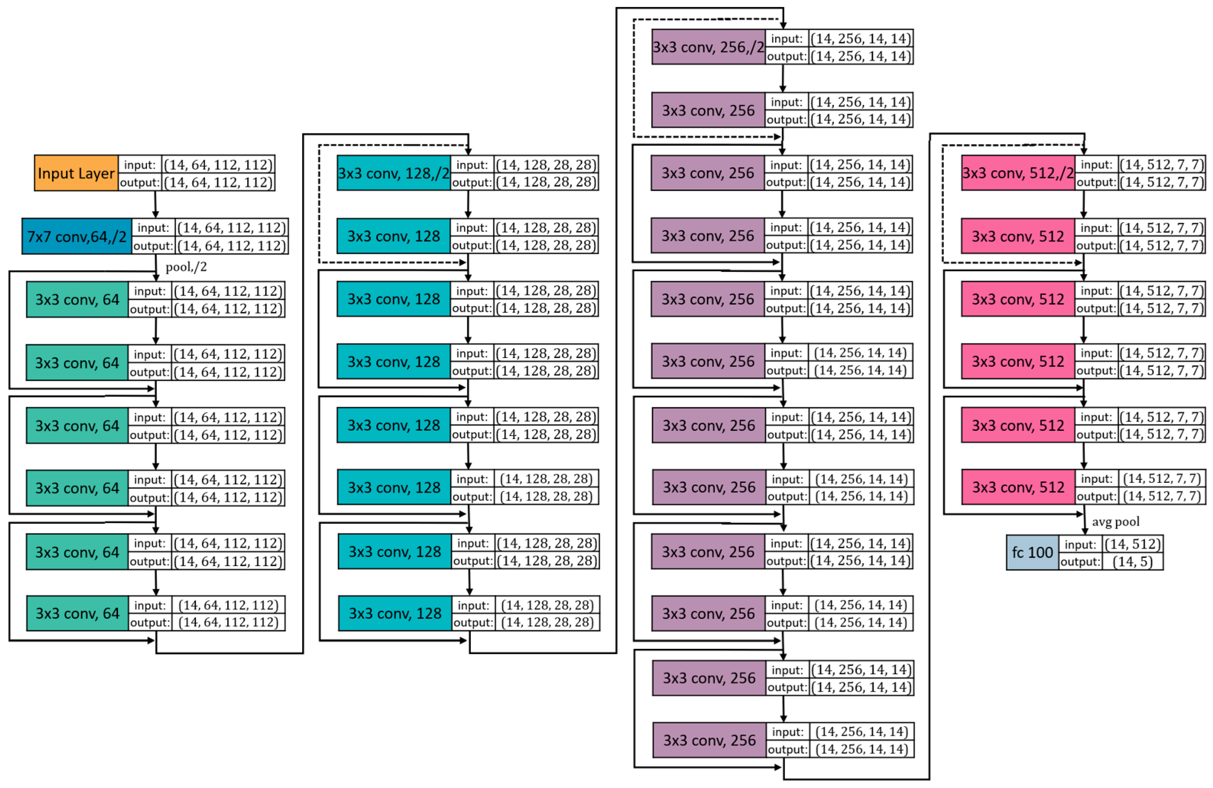
2.2.2. Computational Analysis: ResNet34 NN
3. Results
3.1. Database Obtained
3.2. Results of Neural Networks
3.2.1. Hyperparameters
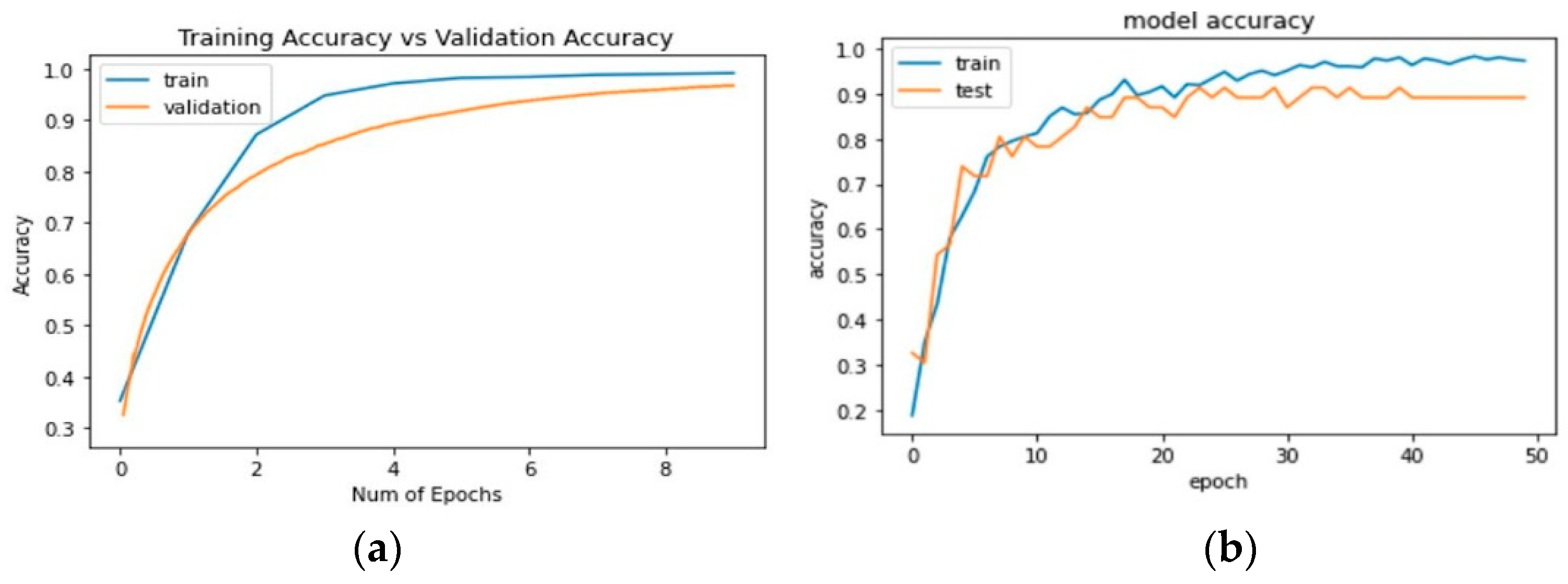
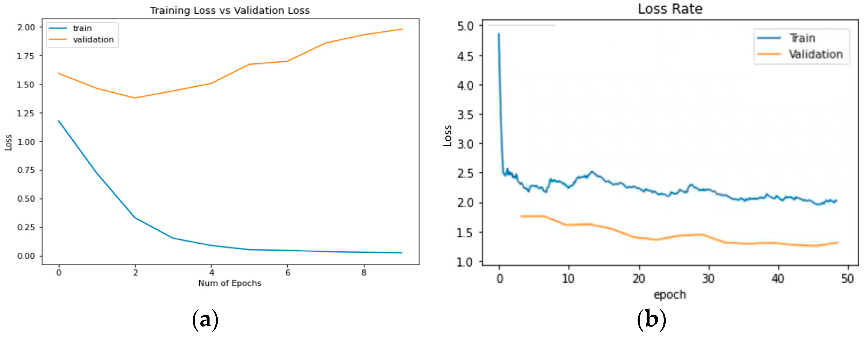
3.2.2. Plots of Learning
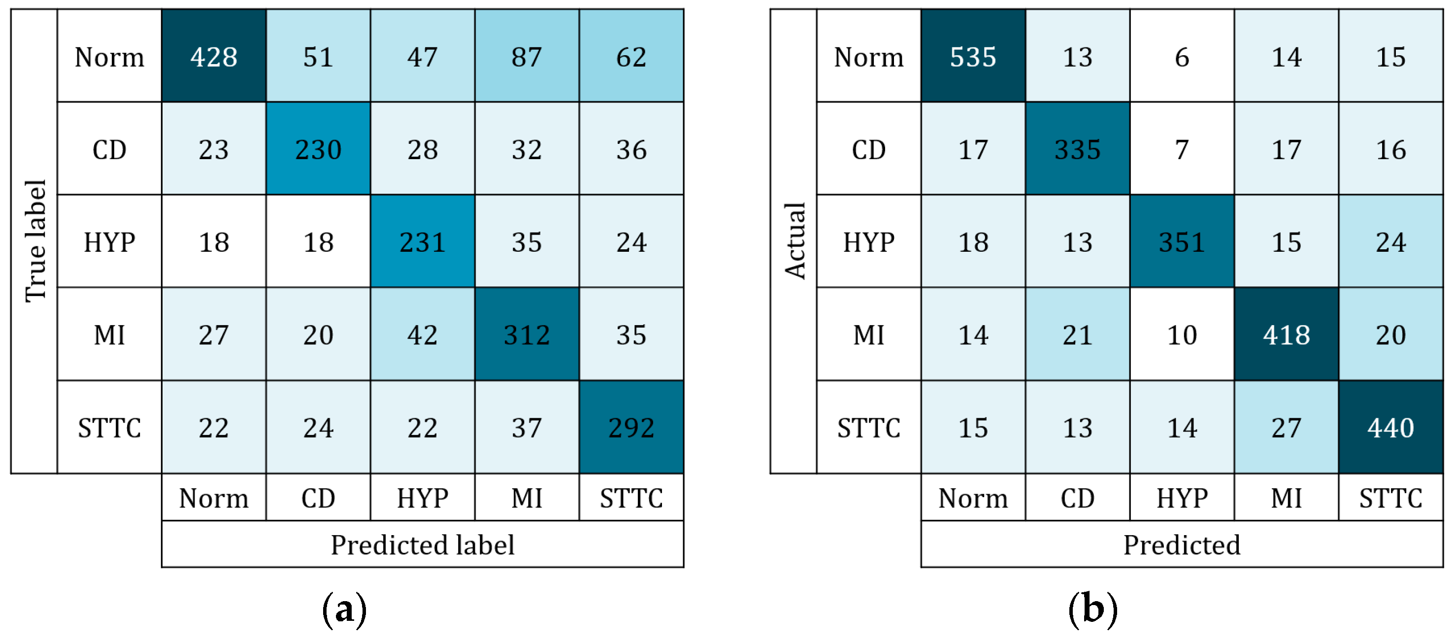
3.2.3. Confusion Matrix
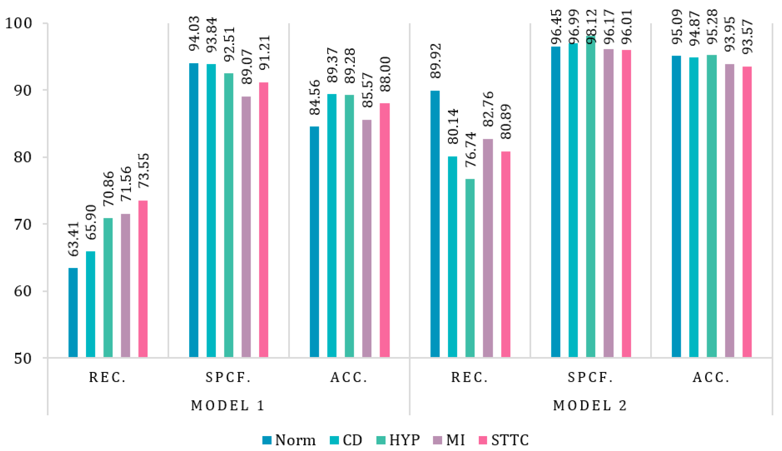
3.2.4. Evaluation Metrics
4. Discussion
- The amount of data in numerical networks is high when standardizing and collecting from several databases or low when using a single database [8].
- Although most apply the classification or detection of pathologies, there is no variety in classes since they are limited to only two.
- The number of channels analyzed is1 or 12, performed with devices at the clinical level; there is no variety in the analysis by channels.
- There are studies in sEMG images, not with sECG images.
- There is a study of electrocardiographic signals with spectrogram images, but it comes back to the issue of channels since there is only one channel.
- There is no database for surface images (sECG, sEMG, sECG, and others), so the images that exist are electromyography images and are limited [37].
5. Conclusions
Author Contributions
Funding
Institutional Review Board Statement
Informed Consent Statement
Data Availability Statement
Conflicts of Interest
References
- WHO. Cardiovascular Diseases (CVDs). Available online: https://www.who.int/news-room/fact-sheets/detail/cardiovascular-diseases-(cvds) (accessed on 28 July 2021).
- MPS. Indicadores Básicos de Salud Ecuador-2012. WHO Statistical Profile. Available online: https://www3.paho.org/ecu/index.php?option=com_docman&view=download&category_slug=documentos-2014&alias=471-indicadores-basicos-de-salud-ecuador-2012&Itemid=599 (accessed on 9 July 2021).
- INEC. Anuario de Estadísticas Vitales—Nacimientos y Defunciones. Available online: https://www.ecuadorencifras.gob.ec/.pdf (accessed on 30 July 2021).
- MSP. MSP Previene Enfermedades Cardiovasculares con Estrategias Para Disminuir Los Factores de Riesgo. Available online: https://www.salud.gob.ec/msp-previene-enfermedades-cardiovasculares-con-estrategias-para-disminuir-los-factores-de-riesgo/ (accessed on 9 July 2021).
- Busnatu, S.S.; Serbanoiu, L.I.; Lacraru, A.E.; Andrei, C.L.; Jercalau, C.E.; Stoian, M.; Stoian, A. Effects of Exercise in Improving Cardiometabolic Risk Factors in Overweight Children: A Systematic Review and Meta-Analysis. Healthcare 2022, 10, 82. [Google Scholar] [CrossRef] [PubMed]
- ECG & Echo Learning. Cardiac Electrophysiology: Action Potential, Automaticity and Vectors. Clinical ECG Interpretation. Available online: https://ecgwaves.com/topic/cardiac-electrophysiology-ecg-action-potential-automaticity-vector/ (accessed on 14 June 2021).
- Williams, L.; Wilkins, P. ECG Interpretation Made Incredibly Easy! 5th ed.; Wolters Kluwer: London, UK, 2011. [Google Scholar]
- Jung, W.H.; Lee, S.G. ECG Identification Based on Non-Fiducial Feature Extraction Using Window Removal Method. Appl. Sci. 2017, 7, 1205. [Google Scholar] [CrossRef] [Green Version]
- Merletti, R.; Muceli, S. Tutorial. Surface EMG Detection in Space and Time: Best Practices. J. Electromyogr. Kinesiol. 2019, 49, 102363. [Google Scholar] [CrossRef] [PubMed]
- Merletti, R.; Botter, A.; Troiano, A.; Merlo, E.; Alessandro, M. Technology and Instrumentation for Detection and Conditioning of the Surface Electromyographic Signal: State of the Art. Clin. Biomech 2009, 24, 122–134. [Google Scholar] [CrossRef] [PubMed]
- Urbanek, H.; van der Smagt, P. IEMG: Imaging Electromyography. J. Electromyogr. Kinesiol. 2016, 27, 1–9. [Google Scholar] [CrossRef]
- Shin, H.; Zheng, Y.; Hu, X. Variation of Finger Activation Patterns Post-Stroke Through Non-Invasive Nerve Stimulation. Front. Neurol. 2018, 9, 1101. [Google Scholar] [CrossRef]
- Geng, W.; Du, Y.; Jin, W.; Wei, W.; Hu, Y.; Li, J. Gesture Recognition by Instantaneous Surface EMG Images. Sci. Rep. 2016, 6, 6–13. [Google Scholar] [CrossRef]
- Shaw, L.; Bagha, S. Online Emg Signal Analysis for Diagnosis of Neuromuscular Diseases By Using Pca and Pnn. Int. J. Eng. Sci. 2012, 4, 4453–4459. [Google Scholar]
- Kachuee, M.; Fazeli, S.; Sarrafzadeh, M. ECG Heartbeat Classification: A Deep Transferable Representation. In Proceedings of the 2018 IEEE International Conference on Healthcare Informatics (ICHI), New York, NY, USA, 4–7 June 2018; pp. 443–444. [Google Scholar] [CrossRef] [Green Version]
- Saadatnejad, S.; Oveisi, M.; Hashemi, M. LSTM-Based ECG Classification for Continuous Monitoring on Personal Wearable Devices. IEEE J. Biomed. Health Inform. 2020, 24, 515–523. [Google Scholar] [CrossRef] [Green Version]
- Ardan, A.N.; Ma’arif, M.; Aisyah, Z.H.; Olivia, M.; Titin, S.M. Myocardial Infarction Detection System from PTB Diagnostic ECG Database Using Fuzzy Inference System for S-T Waves. J. Phys. Conf. Ser. 2019, 1204, 012071. [Google Scholar] [CrossRef]
- Jian, J.Z.; Ger, T.R.; Lai, H.H.; Ku, C.M.; Chen, C.A.; Abu, P.A.R.; Chen, S.L. Detection of Myocardial Infarction Using Ecg and Multi-Scale Feature Concatenate. Sensors 2021, 21, 1906. [Google Scholar] [CrossRef]
- Granados, J.; Westerlund, T.; Zheng, L.; Zou, Z. IoT Platform for Real-Time Multichannel ECG Monitoring and Classification with Neural Networks. In Proceedings of the International Conference on Research and Practical Issues of Enterprise Infor-mation Systems, Shanghai, China, 18–20 October 2017; 2018; 310, pp. 181–191. [Google Scholar] [CrossRef]
- Darmawahyuni, A.; Nurmaini, S.; Sukemi; Caesarendra, W.; Bhayyu, V.; Rachmatullah, M.N.; Firdaus. Deep Learning with a Recurrent Network Structure in the Sequence Modeling of Imbalanced Data for ECG-Rhythm Classifier. Algorithms 2019, 12, 118. [Google Scholar] [CrossRef] [Green Version]
- Topalović, I.; Graovac, S.; Popović, D.B. EMG Map Image Processing for Recognition of Fingers Movement. J. Electromyogr. Kinesiol. 2019, 49, 102364. [Google Scholar] [CrossRef]
- Moin, A.; Zhou, A.; Rahimi, A.; Benatti, S.; Menon, A.; Tamakloe, S.; Ting, J.; Yamamoto, N.; Khan, Y.; Burghardt, F.; et al. An EMG Gesture Recognition System with Flexible High-Density Sensors and Brain-Inspired High-Dimensional Classifier. In Proceedings of the 2018 IEEE International Symposium on Circuits and Systems (ISCAS), Florence, Italy, 27–30 May 2018; pp. 1–5. [Google Scholar] [CrossRef] [Green Version]
- Physionet. PTB-XL, a Large Publicly Available Electrocardiography Dataset v1.0.1. Available online: https://physionet.org/content/ptb-xl/1.0.1/ (accessed on 11 August 2021).
- Wagner, P.; Strodthoff, N.; Bousseljot, R.D.; Kreiseler, D.; Lunze, F.I.; Samek, W.; Schaeffter, T. PTB-XL, a Large Publicly Available Electrocardiography Dataset. Sci. Data 2020, 7, 154. [Google Scholar] [CrossRef]
- Mandellos, G.J.; Koukias, M.N.; Styliadis, I.S.; Lymberopoulos, D.K. E-SCP- ECG + Protocol: An Expansion on SCP-ECG Protocol for Health Telemonitoringpilot Implementation. Int. J. Telemed. Appl. 2010, 2010, 1–17. [Google Scholar] [CrossRef] [Green Version]
- Aguiar, E. Eviaguiar/Detection-of-Cardiac-Pathologies-by-Neural-Networks: Detection of Cardiac Pathologies by Neural Networks. Repository 2022. Available online: https://doi.org/10.5281/ZENODO.6459733 (accessed on 14 April 2022).
- Raponi, M. Programación en MATLAB: Procesamiento Digital de Imágenes. TDI—UNSAM. 2006. Available online: http://www.unsam.edu.ar/escuelas/ciencia/alumnos/tutorial_matlab_tdi.pdf (accessed on 14 April 2022).
- Databricks. DeepLearningECGs. Available online: https://databricks.com/notebooks/iot-medical/deep-learning.htm (accessed on 9 September 2021).
- Huang, C.; Tang, J.; Niu, Y.; Cao, J. Enhanced bifurcation results for a delayed fractional neural network with heterogeneous orders. Phys. A Stat. Mech. Appl. 2019, 526, 121014. [Google Scholar] [CrossRef]
- Xu, C.; Zhang, W.; Aouiti, C.; Liu, Z.; Liao, M.; Li, P. Further investigation on bifurcation and their control of fractional-order bidirectional associative memory neural networks involving four neurons and multiple delays. Math. Methods Appl. Sci. 2021, 1–24. [Google Scholar] [CrossRef]
- Li, Y.; Zhang, Y.; Cai, Y. A New Hyper-Parameter Optimization Method for Power Load Forecast Based on Recurrent Neural Networks. Algorithms 2021, 14, 163. [Google Scholar] [CrossRef]
- Xu, C.; Liao, M.; Li, P.; Guo, Y.; Liu, Z. Bifurcation Properties for Fractional Order Delayed BAM Neural Networks. Cognitive Computation 2021, 13, 322–356. [Google Scholar] [CrossRef]
- Merone, M.; Soda, P.; Sansone, M.; Sansone, C. ECG Databases for Biometric Systems: A Systematic Review. Expert Syst. Appl. 2017, 67, 189–202. [Google Scholar] [CrossRef]
- Bond, R.R.; Finlay, D.D.; Nugent, C.D.; Moore, G. A Review of ECG Storage Formats. Int. J. Med. Inform. 2011, 80, 681–697. [Google Scholar] [CrossRef] [PubMed]
- Gao, M.; Chen, J.; Mu, H.; Qi, D. A Transfer Residual Neural Network Based on Resnet-34 for Detection of Wood Knot Defects. Forests 2021, 12, 212. [Google Scholar] [CrossRef]
- Rubin, J.; Parvaneh, S.; Rahman, A.; Conroy, B.; Babaeizadeh, S. Densely Connected Convolutional Networks and Signal Quality Analysis to Detect Atrial Fibrillation Using Short Single-Lead ECG Recordings. Comput. Cardiol. 2017, 44, 1–4. [Google Scholar] [CrossRef]
- Phinyomark, A.; Scheme, E. EMG Pattern Recognition in the Era of Big Data and Deep Learning. Big Data Cogn. Comput. 2018, 2, 1–27. [Google Scholar] [CrossRef] [Green Version]


| AI | Application | Type of Leads | Ref. |
|---|---|---|---|
| NN | ECG heartbeat classification | 1 lead II ECG | [15] |
| NN | ECG continuous monitoring | single channel ECG signal | [16,17] |
| ML | Detection of MI | 12 channels ECG bipolar and unipolar | [18,19] |
| NN | MI and Norm condition classification | 15 channels ECG bipolar and unipolar | [20] |
| ML | EMG signal of finger movement detection | images sEMG of 24 channels | [21] |
| ML | EMG signal of finger movement detection | images sEMG of 64 channels | [22] |
| NN | EMG gesture recognition | images sEMG of 129 channels | [13] |
| ID | Name | Records |
|---|---|---|
| NORM | Normal ECG | 2682 |
| CD | Conduction Disturbance | 2009 |
| HYP | Hypertrophy | 2083 |
| MI | Myocardial Infarction | 2538 |
| STTC | ST/T Change | 2406 |
| TOTAL | 11,718 | |
| Norm-Patient 5803 | CD-Patient 2044 | HYP-Patient 25 | MI-Patient 1124 | STTC-Patient 9765 |
|---|---|---|---|---|
 | 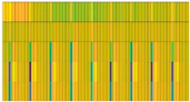 |  | 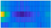 | 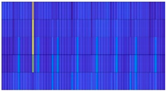 |
| Hyperparameters | Epoch Number | Time of Training | Batch Size | Learning Rate | # Layers | Activation Function | Optimizer | # Training Dataset | # Validation Dataset |
|---|---|---|---|---|---|---|---|---|---|
| LSTM | 12 | ~4 h | 500 | 1 × 10⁻³ | 9 | SoftMax | Adam | 9535 (82%) | 2183 (18%) |
| ResNet34 | 48 | ~2.5 h | 14 | 1 × 10⁻³ | 48 | ReLU | 9331 (80%) | 2387 (20%) |
| Method | Environment Used | Metrics (%) | Errors | |||
|---|---|---|---|---|---|---|
| Acc. | Rec. | Spcf. | Type I | Type II | ||
| LSTM NN | CPU | 98.71 | 89.06 | 92.13 | 437 | 230 |
| ResNet34 | GPU | 93.65 | 89.64 | 93.42 | 147 | 162 |
| Method | Application | # Parameters | Metrics (%) | Ref. | |||
|---|---|---|---|---|---|---|---|
| Rec. | Spcf. | Acc. | |||||
| Numerical data | LSTM NN Present work | Classification of Norm, CD, HYP, MI, and STTC | 11,718 records of 6 precordial leads | 89.06 | 92.13 | 98.71 | - |
| Deep residual CNN | ECG heartbeat classification | 290 records of lead II | 95.10 | - | 95.90 | [15] | |
| LSTM and algorithms | Continuous cardiac monitoring | ~50,000 records of single channel ECG signal | 99.20 | 93.00 | 99.20 | [16] | |
| LSTM and algorithms | Classification MI and Norm condition | 12,359 records of 15 leads | 98.49 | 97.97 | - | [20] | |
| FIS (ANN) and algorithms | Classification MI and Norm condition | 200 records of single channel ECG signal | 73.00 | - | - | [17] | |
| N-Net | Detection of MI | 240 records of 12 leads | - | - | 95.76 | [18] | |
| MSN-Net | Detection of MI | 240 records of 12 leads | - | - | 61.82 | [18] | |
| Images data | ResNet34 Present work | Classification of Norm, CD, HYP, MI, and STTC | 11,718 sECG images of 6 precordial leads | 89.64 | 93.42 | 93.65 | - |
| KNN | Detection EMG signal of finger movements | 240 images sEMG of 24 channels | - | 95.70 | 97.70 | [21] | |
| HD | Detection EMG signal of finger movements | 30 images sEMG of 64 channels | - | - | 96.64 | [22] | |
| Deep CNN | Gesture recognition | 79 images sEMG of 129 channels | - | 96.70 | 65.10 | [13] | |
| SQI with dense CNN | Classifier AF from normal sinus rhythm, other rhythms, and noise | 8528 spectrograms of single channel ECG signal | - | - | 80.00 | [36] | |
Publisher’s Note: MDPI stays neutral with regard to jurisdictional claims in published maps and institutional affiliations. |
© 2022 by the authors. Licensee MDPI, Basel, Switzerland. This article is an open access article distributed under the terms and conditions of the Creative Commons Attribution (CC BY) license (https://creativecommons.org/licenses/by/4.0/).
Share and Cite
Aguiar-Salazar, E.; Villalba-Meneses, F.; Tirado-Espín, A.; Amaguaña-Marmol, D.; Almeida-Galárraga, D. Rapid Detection of Cardiac Pathologies by Neural Networks Using ECG Signals (1D) and sECG Images (3D). Computation 2022, 10, 112. https://doi.org/10.3390/computation10070112
Aguiar-Salazar E, Villalba-Meneses F, Tirado-Espín A, Amaguaña-Marmol D, Almeida-Galárraga D. Rapid Detection of Cardiac Pathologies by Neural Networks Using ECG Signals (1D) and sECG Images (3D). Computation. 2022; 10(7):112. https://doi.org/10.3390/computation10070112
Chicago/Turabian StyleAguiar-Salazar, Evelyn, Fernando Villalba-Meneses, Andrés Tirado-Espín, Daniel Amaguaña-Marmol, and Diego Almeida-Galárraga. 2022. "Rapid Detection of Cardiac Pathologies by Neural Networks Using ECG Signals (1D) and sECG Images (3D)" Computation 10, no. 7: 112. https://doi.org/10.3390/computation10070112
APA StyleAguiar-Salazar, E., Villalba-Meneses, F., Tirado-Espín, A., Amaguaña-Marmol, D., & Almeida-Galárraga, D. (2022). Rapid Detection of Cardiac Pathologies by Neural Networks Using ECG Signals (1D) and sECG Images (3D). Computation, 10(7), 112. https://doi.org/10.3390/computation10070112