A Comparative Study on Denoising Algorithms for Footsteps Sounds as Biometric in Noisy Environments

Abstract

Biometrics is the automated identification of a person based on distinctive characteristics, such as fingerprints, face, voice, or the sound of footsteps. This last characteristic has significant challenges considering the background noise present in any real-life application, where microphones would record footsteps sounds and different types of noise. For this reason, it is crucial to consider not only the capacity of classification algorithms for recognizing a person using foostetps sounds, but also at least one stage of denoising algorithms that can reduce the background sounds before the classification. In this paper we study the possibilities of a two-stage approach for this problem: a denoising stage followed by a classification process. The work focuses on discovering the proper strategy for applying combinations of both stages for specific noise types and levels. Results vary according to the type and level of noise, e.g., for White noise at signal-to-noise ratio level, accuracy can increase from 0.96 to 1.00 by applying deep learning based-filters, but the same option does not benefit the cases of signals with low level natural noises, where Wiener filtering can increase accuracy from 0.6 to 0.77 at the highest level of noise. The results represent a baseline for developing real-life implementations of footstep biometrics.

1. Introduction

The purpose of biometrics is the identification of an individual using biological or physical measurement that can be related to a unique person. For example, the use of fingerprints had been employed by criminologists since the 19th century, but it was not until the second part of the 20th century that technology allowed the automation of the identification using this characteristic [1].

Other than criminology, the first commercial application of biometrics was the regulated access to buildings, where only a few persons were allowed to enter for security reasons; thus the correct identification of such persons is an essential concern. The most common elements used for this purpose are fingerprints. More recently, other measurements, such as faces and iris recognition have been applied in smartphones [2] and airports [3].

Any measurements of individuals that can allow a proper and unique identification can likely be considered for biometrics. The two main categories considered in the literature, and the most representative measures are [4]: physiological (fingerprints, iris, face) and behavioral (voice, signature recognition, keystroke dynamics, footsteps). Each biometrics has its challenges and possibilities, and recent research that analyzes and provides robustness to existing systems can be found in the literature [5,6].

The case of using footsteps patterns to recognize an individual has a short history, from the first proposals [7] to validation using a proper dataset [8] about thirty-five years ago. The footsteps can be measured and analyzed using several approaches, combining sensors and classification systems [9].

Similar to other biometrics, increasing attention from several research groups arose in recent years [10,11], and similar to other measures, some concerns on practicality and privacy have been reported [12]. For these reasons, several sensing of the phenomenon like vision, sound, pressure, and accelerometry has been explored [13]. The benefits of an application that is based on footsteps recognition can be used in medicine (monitoring and assessment of Parkinson’s disease), physiotherapy (evaluation of recovery from injuries), security, and smarthomes [9,14].

Using sound measures of footsteps to determine a person’s identity is a challenging possibility, given the continuous presence of noise and background sounds present in any real-life application. But the use of sole sounds can represent an advantage given the simplicity and low cost of a sound sensor.

Related Work

The reports on the accuracy of footstep biometrics can be above 90% [3], using sensors from smart floors, video cameras, microphones, or accelerometers. It is important to remark that the accuracy of a system should be considered carefully for comparison purposes, given the wide range of possibilities where experiments are performed. For example, not only the sensing methods can be different, but the classes considered as well: identifying one person among two possibilities (binary case), one person among several, known versus unknown person, an individual in a crowd, etc. Additionally, the system’s performance can be affected by other factors like the types of footwear worn and the different kinds of floors [11,15].

The case of using distant sound recording as the sole form of identification for individuals, has been explored in the past years. The first research on multiple persons using this source of information was published in [16]. For this purpose, characteristic parametrization of sounds, such as spectral features was applied to analyze the signals.

The incorporation of feature selection methods plays an important role in many machine learning application, as shown in recent sound-based classification [17,18] and new robust biometrics [19]. In this work, we focus on analysing sounds of footsteps registered using a distant microphone in the presence of additive noise, and the mandatory denoising methods required for the classification process. A fixed number of features were selected, according to the possibilities of the implementation. Our goal is the exploration of denoising algorithms in combination with classification methods, to establish the capability of a biometrics system.

The study’s novelty relies on its focus on the extensive consideration of noise as an unavoidable part of the real-life implementation of footstep sounds as biometrics and the quantitative evaluation of a large set of conditions for this purpose. The rest of the paper is organized as follows: Section 2 presents the Material and Methods used for the Footstep sound analysis. Section 3 presents the results. Section 4 summarizes the discussion, and finally, Section 5 presents the Conclusions.

2. Materials and Methods

This section presents the recording conditions and analysis of the sound signals performed to establish the experiments, which combine denoising and classification algorithms.

2.1. Footsteps Sound Analysis

Footsteps can be analyzed and represented in several domains using a range of conditions and sensing methods.

In our work, we employ temporal and spectral features to characterize the sound signals. For this purpose, the pyAudioAnalysis tool [20] was applied to extract the features suitable for the application of classification algorithms. The extracted features using the pyAudioAnalysis are:

• Zero Crossing Rate: Defined as [21]

  $$ZCR=\sum _{m=-\infty }^{\infty }|sgn\left(x\left(m\right)\right)-sgn\left(x(m-1)\right)|w(n-m),$$

  (1)

  where $sng\left(x\right)$ is the sign function, and $w\left(n\right)$ is $\frac{1}{2N}$ for $0<n<N-1$. This is a measure of the rate of the sign changes, and has been applied in other sound-based tasks, such as Voice Activity Detection.
• Energy: The energy of the signal can be computed using the sum of squares of the signal samples, following the equation:

  $$E\left(x\left(n\right)\right)=\sum _{n=-\infty }^{\infty }{\left|x\left(n\right)\right|}^2.$$

  (2)
• Entropy of Energy: The entropy of the energy is also important as a measure of abrupt changes in the energy of frames.
• Spectral Centroid: This is a measure that represents the center of mass of the signal’s spectrum.
• Spectral Spread: Is a measure of the variance in the signal’s spectrum.
• Spectral Entropy: The entropy can be measured in the spectrum, quantifying the spectral complexity of the speech signal. It can be obtained by [22]

  $$SE=\sum _f{p}_{f}log\frac{1}{p_f},$$

  (3)

  where $p_f$ is each frequency.
• Spectral Flux: This is a measure of how quickly the spectrum is changing, by calculating the square of successive frames.
• Spectral Rolloff: It is the frequency below which 90% of the energy of the spectrum is concentrated.
• Mel Frequency Cepstral Coefficients (MFCCs): It is a representation of the power spectrum, based on the Fourier Transform mapped on the nonlinear mel scale of frequency. MFCCs vectors are commonly applied in speech recognition tasks. A detailed description of the MFCC can be found in [23].
• Chroma Vector: Chroma vectors are a representation of the spectrum, mapped into the twelve pitch classes of the traditional tonal music.
• Chroma Deviation: This is the measure of the standard deviation of the chroma coefficients.

2.2. Experimental Setup

The identification of persons using footstep sounds has inherently a wide range of possibilities. For this reason, the experimental conditions have to be chosen carefully, in order to delimit the study in defined directions. For this purpose, we have chosen the following conditions to perform the comparative study on denoising algorithms for footstep sounds as biometric:

• Binary classification: The binary case of classification was defined for this experiments. This means that the data comes from the recording of two persons, and the identification pretends to distinguish between one of two possibilities.
• Noise: As mentioned in the Introduction, the presence of noise has to be contemplated in any real-file scenario of sound recording and processing. For our experiments, we consider both naturally and artificially generated noise. The Babble and Office Noise, obtained from mynoise.net accessed on 12 February 2022 provides realistic scenarios where a biometrics system could be implemented. On the other hand, White noise is usually analyzed in signal denoising tasks. For every type of noise, we add five signal-to-noise ratio (SNR) levels (−10, −5, 0, 5, 10) to cover light to heavy noise affectation of the footsteps sound signals.
• Denoising Algorithms: The problem of denoising signals has been explored for decades, and the comparison of algorithms is a usual task in sound-enhancing experiences. For this experimental setup, we chose three of the most commonly applied algorithms based on classical signal processing, along with a deep learning-based approach. Details of the algorithms are presented in Section 2.2.2.
• Classifiers: For this first experience of exploring the functionality of a system based on classification and denoising algorithms, we chose the Support Vector Machines (SVM) classifier. From the implementation in pyAudioAnalysis, a cross-validation procedure is performed to select the parameters for the optimal classifiers, like the margin parameter C for the SVM.

2.2.1. Dataset

In our experiments, we developed a dataset of footstep sounds registered using a distant microphone. For this purpose two female volunteer participants were recorded in several sessions, using a single Omni-directional microphone AKG C414 XLII. Both participants walked naturally around the microphone, describing a circle of about 1.5 m. A laboratory space at the University of Costa Rica was conditioned for the experiments. Figure 1 shows the setup of the recording sessions.

The volunteers were asked to walk using a natural pace, and fifteen minutes of footsteps sounds were recorded in each session, using WAV files with a sampling of 44,100 Hz and 16 bits. The best recordings, in terms of continuity and lack of additional transient sounds were selected for the second step of processing and editing.

The audio files of the recording sessions were post-processed and edited to obtain segments of five seconds with steps sound. The duration was defined in order to provide the classifiers with data of several footsteps each time, and with the first footstep not necessarily located at the beginning of the audio.

The focus of this work is on the numerical analysis of how noise affects the identification process modeling it as an additive process. Further studies must take into account the homogenization of other conditions such as the type of shoes, the floor material, the similar weight of participants, among other factors.

2.2.2. Sound Classification in Noisy Environments

The Experimental Setup was defined to simulate the real-life application of distant sound of footsteps as biometrics. For this purpose, the presence of several kinds of noise at several levels is an essential part of the study. For each five-second segment of the audio file with footsteps sounds, the five SNR levels of each noise were added.

Then, the recognition’s performances were tested under the assumption that any real-life system should provide a noise filter to preserve the quality of the signal for the classifiers. For this purpose, we selected four open-source implemented filters, described as follows:

1.

MMSE: As usual in several denoising methods, the Minimum Mean Square Error algorithm (MMSE) models the presence of noise as an additive process, as

$$y\left(t\right)=x\left(t\right)+n\left(t\right),$$

(4)

where $y\left(t\right)$ is the noisy signal, composed as the sum of the clean signal $x\left(t\right)$ and the background noise $n\left(t\right)$. In this algorithm, following the implementation from [24], to enhance the signal from a representation of Mel-Frequency Cepstral (MFCC) and DCT Coefficients vectors ($c_y$), the clean coefficients $c_x$ are estimated as

$$\begin{array}{c}\hfill \widehat{c_x}\left(k\right)=E\left\{c_x\left(k\right)|m_y\right\}=\sum _b{a}_{k,b}E\left\{log{m}_x\left(b\right)|m_y\right\},\end{array}$$

(5)

where $a_{k,b}$ are the DCT coefficients, and $m_x$, $m_y$ are the output of the MFCC filter bank, and b the filter channel index. Those parameters are estimated from 39-dimension MFCC coefficients, while making assumptions on the noise models. We chose the parameters according to the solution proposed by [24]. It is important to remark the various selection and weighting methods of DCT coefficient that can be employed and compared, as presented in [19]. An analysis of such relevant procedures can be explored as future work.

2.

Spectral subtraction: Using the same additive noise model of the previous case (Equation (4)), the power spectrum of the noisy speech can be estimated as [25]:

$${\left|Y\left(k\right)\right|}^2\approx {\left|X\left(k\right)\right|}^2+{\left|N\left(k\right)\right|}^2,$$

(6)

where $\left|P\right(k\left)\right|$ is the magnitude of the discrete spectrum of the corresponding noisy speech, the clean version and the noise. The noise spectrum $\hat{N}\left(k\right)$ is approximated from silence segments. In the implementation presented in [25], the clean speech spectrum is estimated as

$$|\hat{X}{\left(k\right)|}^2={\left|Y\left(k\right)\right|}^2-\alpha {\left|\hat{D}\left(k\right)\right|}^2,$$

(7)

where $alpha$ is a coefficient established according to the SNR. This means that its value can be estimated from the corrupted speech signal and the noise measured during segments of silence.

3.

Wiener filter: The Wiener filtering is one of the most successful and commonly implemented algorithms for denoising speech signals. The filtering is performed by minimizing the Mean Square Error. In the description presented in [26], the minimization in the frequency domain can be formulated using the transfer function

$$H\left(\omega \right)=\frac{P_x\left(\omega \right)}{P_x\left(\omega \right)+P_n\left(\omega \right)},$$

(8)

where, $P_x\left(\omega \right)$ is the clean signal power spectrum and $P_n\left(\omega \right)$ is the noise power spectrum. According to the implementation of [27], the enhanced signal can be approximated by

$${\hat{P}}_x\left(\omega \right)=H\left(\omega \right)P_y\left(\omega \right).$$

(9)

where, $P_y\left(\omega \right)$ is the power spectrum of the noisy signal. An estimation of $P_y\left(\omega \right)$ can be obtained during periods of silence.

4.

Deep learning: The application of deep learning-based algorithms for denoising sound signals has been successfully applied in recent experiences. Among the different approaches and types of deep learning models, recurrent neural networks such as Long-short Term Memory (LSTM) stand out for their results and capacity to model sequential information.

For our experiments, we chose the PyTorch implementation of LSTM-based autoencoders presented by Facebook Research (https://github.com/facebookresearch/denoiser, accessed on 12 February 2022). This implementation is based on an encoder/decoder architecture that combines convolutional and LSTM layers, with skip U-net connections. It works with raw waveforms. Further details can be found in [28], where we extracted the parameters of the neural network.

2.2.3. Evaluation

To evaluate each classifier, the set of available data was divided into training and test sets in a proportion of 80% and 20%, respectively. The common measures for assessing the results were calculated in the test set: True positives, True Negatives, False Positives, and False Negatives. With that measure for each case, the typical Accuracy, Precision, Recall and F1-score were obtained. In this work, we focus on the performance of the classifier before and after the denoising process with the different types of algorithms.

Given the impulsive nature of the footsteps sounds in comparison to the background noise, the observation of waveforms and spectrograms is introduced as a means of illustrating the denoising process and the contamination of the signals with the noise, as well as the enhancement achieved with the denoising algorithms.

3. Results

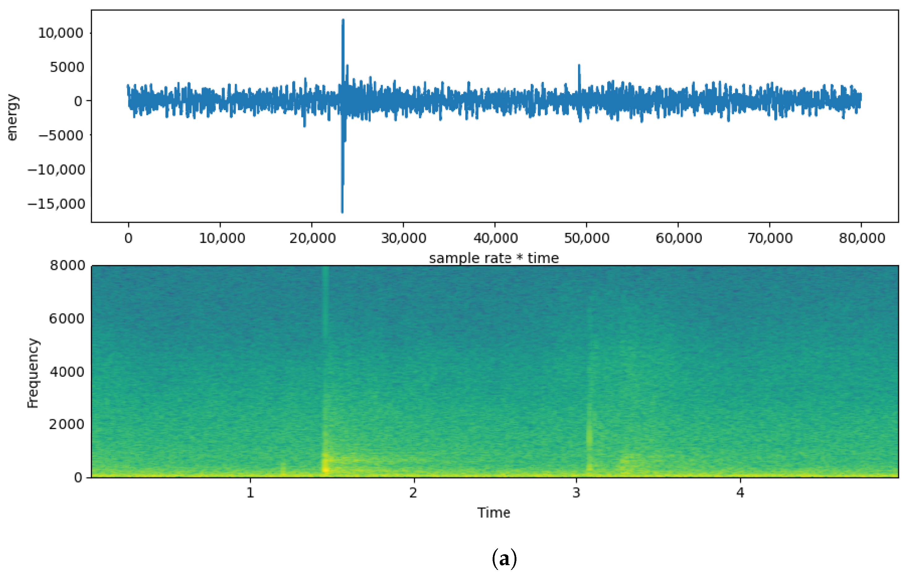
The challenges of a classification process of footsteps in the presence of noise are remarkable in the case of a distant microphone. Figure 2 illustrates the case of White noise with SNR 0. In Figure 2b it is evident how the noise affects the entire spectrum and makes almost unrecognizable the impulses of the footsteps shown in Figure 2a. For traditional algorithms, such degradation may represent a very difficult task, in terms of recovering the original signal. But with the application of deep learning denoising, the impulses became visible again after the denoising, as shown in Figure 2c.

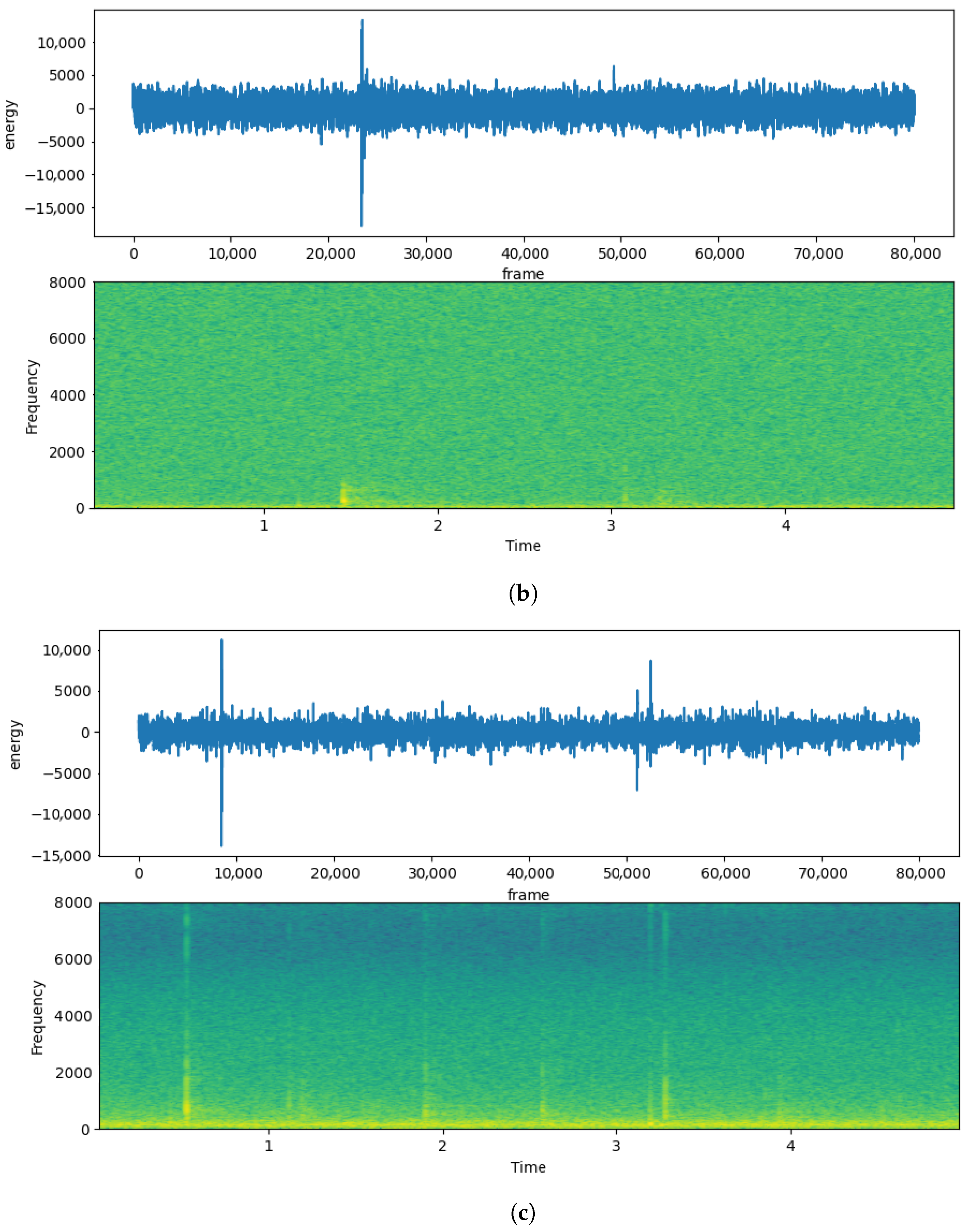
As expected, for the case of a non-stationary, natural noise, such as Babble, the denoising process is not as effective as White noise case, even with the application of deep learning algorithm. Given this observation, it is expected that the classification process with signals degraded with this kind of noise becomes less effective in terms of Accuracy, Precision, Recall, and F1-score (Figure 3).

The availability of data became an important issue for the application of deep learning-based denoising. To keep a proper comparison, the SVM classifier was trained using only the test set of the deep neural network training process. This means that most of the data collected during the recording sessions were used for training and validation of the deep learning denoising process, and only the test set was available for the training of the classifier. The large data requirements are a limitation to consider if a two-stage denoising and classification proposal considers deep learning for both processes.

The detailed results for Babble, White, and Office of our experiments are organized according to the type of noise and level, in Table 1, Table 2, Table 3, Table 4, Table 5, Table 6, Table 7, Table 8, Table 9, Table 10, Table 11, Table 12, Table 13, Table 14 and Table 15. In each table, the classification metrics are reported for the noisy signal and the results of the four denoising algorithms. The first results correspond to Babble SNR-10, in Table 1.

This natural noise, at such high SNR level, affects the performance of the classifier considerably, with an accuracy as low as 0.60 in this binary case. Most of the denoising algorithms did not obtain improvements in any of the classification measures, with the only exception of Wiener filtering.

Table 1. Babble Noise SNR 10. * is the best result for each particular measure.

Algorithm	Accuracy	Precision	Recall	F1-Score
No filter	0.60	0.65	0.59	0.62
MMSE [24]	0.56	0.50	0.57	0.53
Spectral subtraction [25]	0.67	0.58	0.71	0.64
Wiener [27]	0.77 *	0.77 *	0.77 *	0.77 *
Deep learning [28]	0.43	0.40	0.42	0.41

Table 1. Babble Noise SNR 10. * is the best result for each particular measure.

Algorithm	Accuracy	Precision	Recall	F1-Score
No filter	0.60	0.65	0.59	0.62
MMSE [24]	0.56	0.50	0.57	0.53
Spectral subtraction [25]	0.67	0.58	0.71	0.64
Wiener [27]	0.77 *	0.77 *	0.77 *	0.77 *
Deep learning [28]	0.43	0.40	0.42	0.41

A similar situation of poor denoising performance is observed in Table 2. None of the algorithms could enhancing the signal to achieve acceptable accuracy. In fact, proper classification results were obtained from SNR 0 or lower levels, as shown in Table 3, Table 4 and Table 5. For such SNR levels, the application of denoising algorithms may represent a favorable procedure that increases accuracy, precision, and F1-score for SNR 0 and SNR 5. The SNR 10 of Babble seems to impact very slightly the performance of the SVM classifier, and the unfiltered version of the signal is the best option for the biometric identification of the volunteers.

Table 2. Babble Noise SNR −5. * is the best result for each particular measure.

Algorithm	Accuracy	Precision	Recall	F1-Score
No filter	0.75	0.77	0.74	0.75
MMSE [24]	0.65	0.58	0.68	0.63
Spectral subtraction [25]	0.77 *	0.81	0.75	0.78 *
Wiener [27]	0.75	0.85 *	0.71	0.77
Deep learning [28]	0.73	0.55	0.85 *	0.67

Table 2. Babble Noise SNR −5. * is the best result for each particular measure.

Algorithm	Accuracy	Precision	Recall	F1-Score
No filter	0.75	0.77	0.74	0.75
MMSE [24]	0.65	0.58	0.68	0.63
Spectral subtraction [25]	0.77 *	0.81	0.75	0.78 *
Wiener [27]	0.75	0.85 *	0.71	0.77
Deep learning [28]	0.73	0.55	0.85 *	0.67

Table 3. Babble Noise SNR 0. * is the best result for each particular measure.

Algorithm	Accuracy	Precision	Recall	F1-Score
No filter	0.92	0.88	0.96	0.92
MMSE [24]	0.79	0.77	0.80	0.78
Spectral subtraction [25]	0.92	0.92 *	0.92	0.92
Wiener [27]	0.94 *	0.88	1.00 *	0.94 *
Deep learning [28]	0.78	0.55	1.00 *	0.71

Table 3. Babble Noise SNR 0. * is the best result for each particular measure.

Algorithm	Accuracy	Precision	Recall	F1-Score
No filter	0.92	0.88	0.96	0.92
MMSE [24]	0.79	0.77	0.80	0.78
Spectral subtraction [25]	0.92	0.92 *	0.92	0.92
Wiener [27]	0.94 *	0.88	1.00 *	0.94 *
Deep learning [28]	0.78	0.55	1.00 *	0.71

Table 4. Babble Noise SNR 5. * is the best result for each particular measure.

Algorithm	Accuracy	Precision	Recall	F1-Score
No filter	0.96	0.92	1.00 *	0.96
MMSE [24]	0.90	0.85	0.96	0.90
Spectral subtraction [25]	0.98 *	0.96 *	1.00 *	0.98 *
Wiener [27]	0.94	0.92	0.96	0.94
Deep learning [28]	0.88	0.75	1.00 *	0.86

Table 4. Babble Noise SNR 5. * is the best result for each particular measure.

Algorithm	Accuracy	Precision	Recall	F1-Score
No filter	0.96	0.92	1.00 *	0.96
MMSE [24]	0.90	0.85	0.96	0.90
Spectral subtraction [25]	0.98 *	0.96 *	1.00 *	0.98 *
Wiener [27]	0.94	0.92	0.96	0.94
Deep learning [28]	0.88	0.75	1.00 *	0.86

Table 5. Babble Noise SNR 10. * is the best result for each particular measure.

Algorithm	Accuracy	Precision	Recall	F1-Score
No filter	0.96 *	0.92 *	1.00 *	0.96 *
MMSE [24]	0.92	0.85	1.00 *	0.92
Spectral subtraction [25]	0.94	0.92 *	0.96	0.94
Wiener [27]	0.96 *	0.92 *	1.00 *	0.96 *
Deep learning [28]	0.95	0.90	1.00 *	0.95

Table 5. Babble Noise SNR 10. * is the best result for each particular measure.

Algorithm	Accuracy	Precision	Recall	F1-Score
No filter	0.96 *	0.92 *	1.00 *	0.96 *
MMSE [24]	0.92	0.85	1.00 *	0.92
Spectral subtraction [25]	0.94	0.92 *	0.96	0.94
Wiener [27]	0.96 *	0.92 *	1.00 *	0.96 *
Deep learning [28]	0.95	0.90	1.00 *	0.95

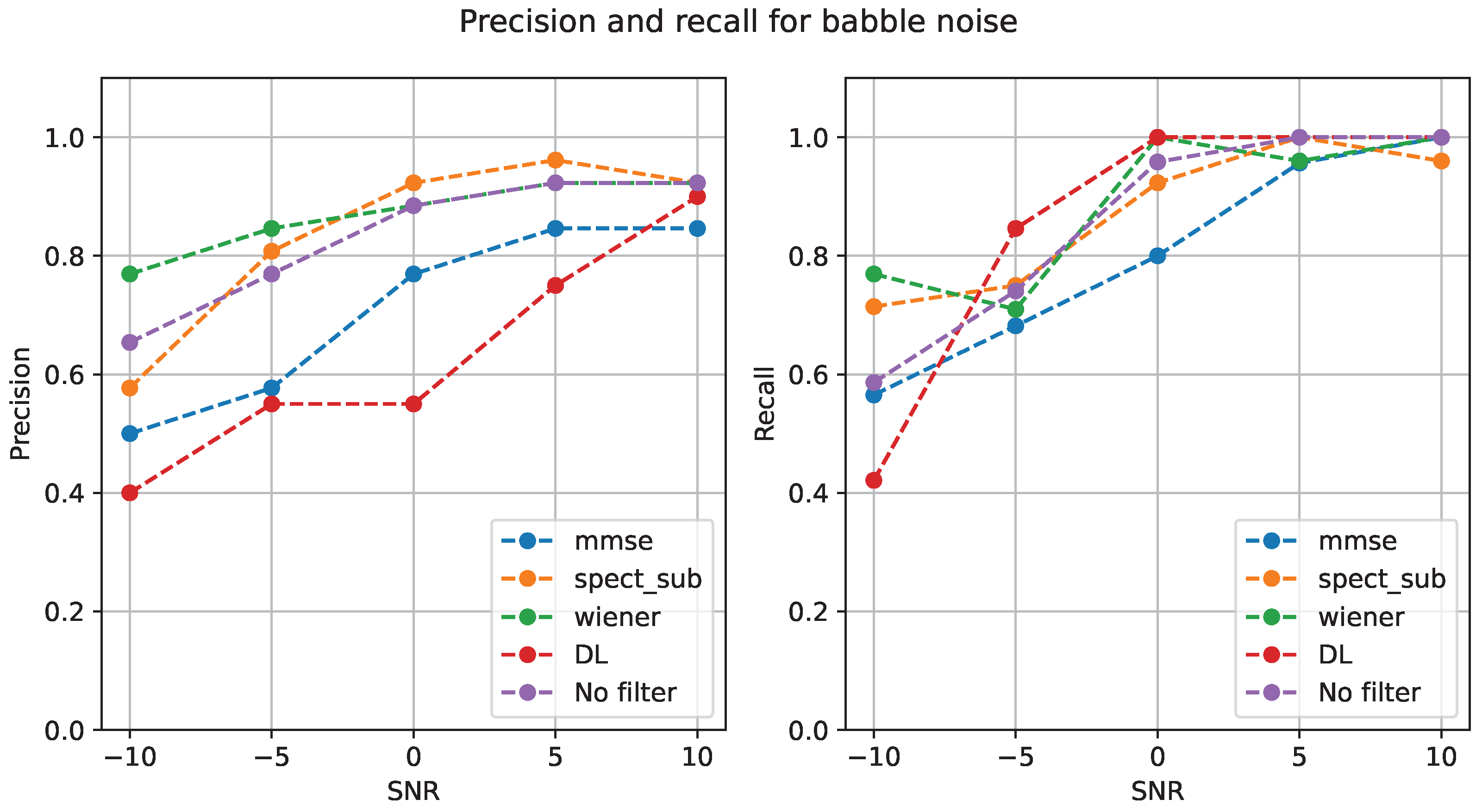
The trend lines of Precision and Recall measures for the case of Babble are presented in Figure 4. It can be observed that some denoising algorithms, such as deep learning and MMSE did not represent any advantage for the process, because the no-filter version of the signal performs better, particularly in terms of Precision. The Recall measure presents fewer differences among the algorithms, with some advantages at the higher level of noise but no significant improvements at SNR 5 or SNR 10.

A very different group of results are presented for the case of White noise, as shown in Table 6, Table 7, Table 8, Table 9 and Table 10. For these results, it seems that the noise does not significantly affect the biometric identification, even for the higher SNR levels. But in every case, deep learning as a denoising algorithm improves the performance of the classification task.

Table 6. White Noise SNR −10. * is the best result for each particular measure.

Algorithm	Accuracy	Precision	Recall	F1-Score
No filter	0.96	0.92	1.00 *	0.96
MMSE [24]	0.92	0.85	1.00 *	0.92
Spectral subtraction [25]	0.88	0.77	1.00	0.87
Wiener [27]	0.94	0.88	1.00 *	0.94
Deep learning [28]	0.98 *	0.95 *	1.00 *	0.97 *

Table 6. White Noise SNR −10. * is the best result for each particular measure.

Algorithm	Accuracy	Precision	Recall	F1-Score
No filter	0.96	0.92	1.00 *	0.96
MMSE [24]	0.92	0.85	1.00 *	0.92
Spectral subtraction [25]	0.88	0.77	1.00	0.87
Wiener [27]	0.94	0.88	1.00 *	0.94
Deep learning [28]	0.98 *	0.95 *	1.00 *	0.97 *

Table 7. White Noise SNR −5. * is the best result for each particular measure.

Algorithm	Accuracy	Precision	Recall	F1-Score
No filter	0.96	0.92	1.00 *	0.96
MMSE [24]	0.96	0.92	1.00 *	0.96
Spectral subtraction [25]	0.96	0.92	1.00 *	0.96
Wiener [27]	1.00 *	1.00 *	1.00 *	1.00 *
Deep learning [28]	1.00 *	1.00 *	1.00 *	1.00 *

Table 7. White Noise SNR −5. * is the best result for each particular measure.

Algorithm	Accuracy	Precision	Recall	F1-Score
No filter	0.96	0.92	1.00 *	0.96
MMSE [24]	0.96	0.92	1.00 *	0.96
Spectral subtraction [25]	0.96	0.92	1.00 *	0.96
Wiener [27]	1.00 *	1.00 *	1.00 *	1.00 *
Deep learning [28]	1.00 *	1.00 *	1.00 *	1.00 *

A relevant observation is that White noise at SNR 0, SNR 5 and SNR 10 does not require filtering, given the perfect performance of the classifier. But, unlike the other denoising algorithms, deep learning application does not affect the performance.

The drop in recognition accuracy with the application of MMSE, Spectral subtraction and Wiener filtering can be explained by the indiscriminate filtering of footsteps information alongside the noise or some introduced distortions, that were not present with deep learning.

Table 8. White Noise SNR 0. * is the best result for each particular measure.

Algorithm	Accuracy	Precision	Recall	F1-Score
No filter	1.00 *	1.00 *	1.00 *	1.00 *
MMSE [24]	0.96	0.92	1.00 *	0.96
Spectral subtraction [25]	0.96	0.92	1.00 *	0.96
Wiener [27]	0.98	0.96	1.00 *	0.98
Deep learning [28]	1.00 *	1.00 *	1.00 *	1.00 *

Table 8. White Noise SNR 0. * is the best result for each particular measure.

Algorithm	Accuracy	Precision	Recall	F1-Score
No filter	1.00 *	1.00 *	1.00 *	1.00 *
MMSE [24]	0.96	0.92	1.00 *	0.96
Spectral subtraction [25]	0.96	0.92	1.00 *	0.96
Wiener [27]	0.98	0.96	1.00 *	0.98
Deep learning [28]	1.00 *	1.00 *	1.00 *	1.00 *

Table 9. White Noise SNR 5. * is the best result for each particular measure.

Algorithm	Accuracy	Precision	Recall	F1-Score
No filter	1.00 *	1.00 *	1.00 *	1.00 *
MMSE [24]	0.98	0.96	1.00 *	0.98
Spectral subtraction [25]	0.98	0.96	1.00 *	0.98
Wiener [27]	0.96	0.92	1.00 *	0.96
Deep learning [28]	1.00 *	1.00 *	1.00 *	1.00 *

Table 9. White Noise SNR 5. * is the best result for each particular measure.

Algorithm	Accuracy	Precision	Recall	F1-Score
No filter	1.00 *	1.00 *	1.00 *	1.00 *
MMSE [24]	0.98	0.96	1.00 *	0.98
Spectral subtraction [25]	0.98	0.96	1.00 *	0.98
Wiener [27]	0.96	0.92	1.00 *	0.96
Deep learning [28]	1.00 *	1.00 *	1.00 *	1.00 *

Table 10. White Noise SNR 10. * is the best result for each particular measure.

Algorithm	Accuracy	Precision	Recall	F1-Score
No filter	1.00 *	1.00 *	1.00 *	1.00 *
MMSE [24]	0.96	0.92	1.00 *	0.96
Spectral subtraction [25]	0.96	0.92	1.00 *	0.96
Wiener [27]	0.98	0.96	1.00 *	0.98
Deep learning [28]	1.00 *	1.00 *	1.00 *	1.00 *

Table 10. White Noise SNR 10. * is the best result for each particular measure.

Algorithm	Accuracy	Precision	Recall	F1-Score
No filter	1.00 *	1.00 *	1.00 *	1.00 *
MMSE [24]	0.96	0.92	1.00 *	0.96
Spectral subtraction [25]	0.96	0.92	1.00 *	0.96
Wiener [27]	0.98	0.96	1.00 *	0.98
Deep learning [28]	1.00 *	1.00 *	1.00 *	1.00 *

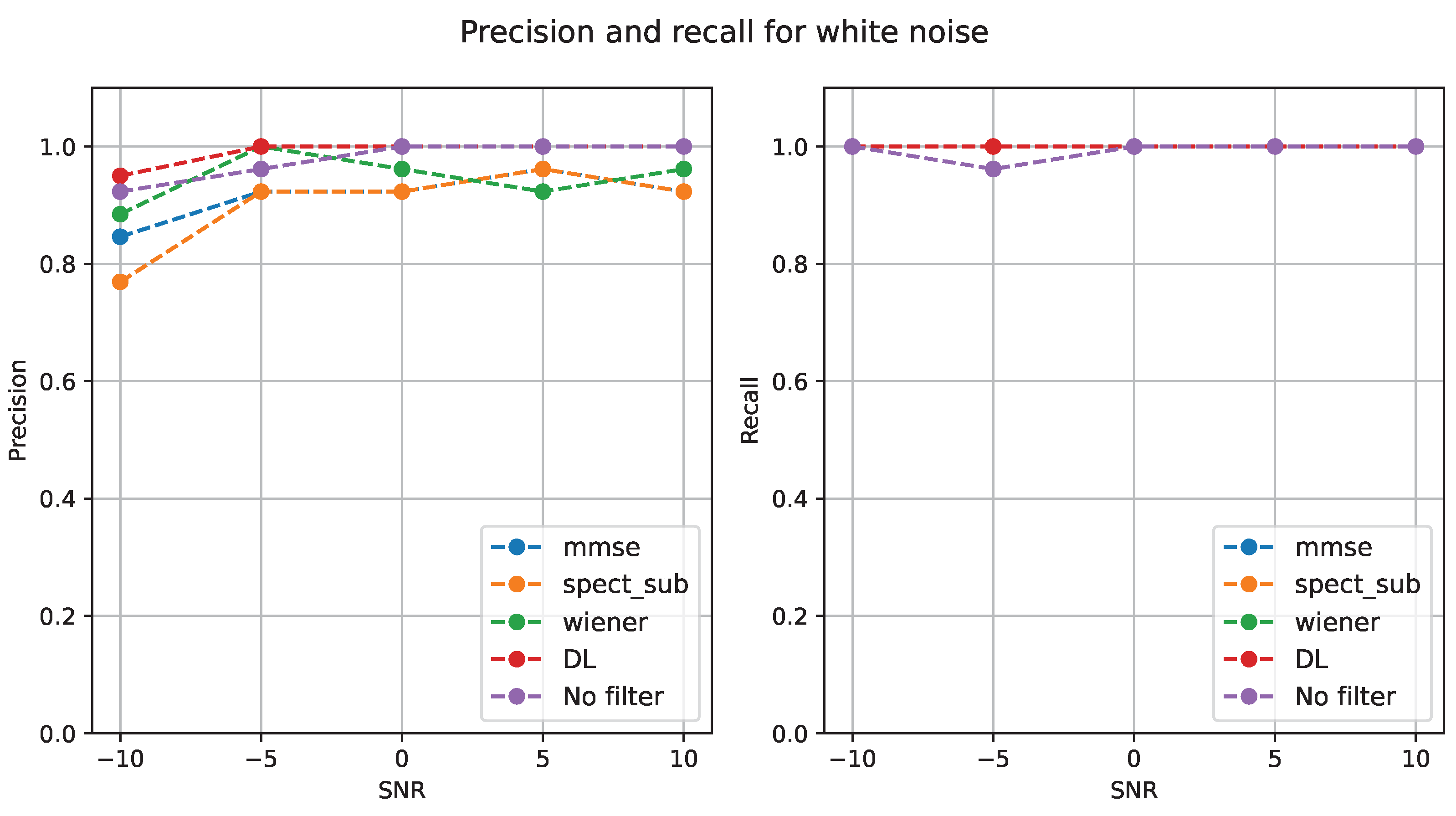
The trend lines of Precision and Recall shown in Figure 5 illustrate the benefit of the deep learning denoising, but the non-need for denoising in SNR 0 or lower levels.

The previous results differ from the last case analyzed: the natural Office noise. The measures for the classification task are shown from Table 11, Table 12, Table 13, Table 14 and Table 15. The noise effect on the person’s identification is evident from accuracy as low as 60% or 75% for the case of SNR −10 and SNR −5. Denoising algorithms of Spectral subtraction and Wiener seems to benefit the process, but were incapable of achieving high enough results to consider them for a real-life application of a biometric system.

Table 11. Office Noise SNR −10. * is the best result for each particular measure.

Algorithm	Accuracy	Precision	Recall	F1-Score
No filter	0.60	0.65	0.59	0.62
MMSE [24]	0.56	0.50	0.57	0.53
Spectral subtraction [25]	0.67	0.58	0.71	0.64
Wiener [27]	0.71 *	0.73 *	0.70 *	0.72 *
Deep learning [28]	0.65	0.65	0.65	0.65

Table 11. Office Noise SNR −10. * is the best result for each particular measure.

Algorithm	Accuracy	Precision	Recall	F1-Score
No filter	0.60	0.65	0.59	0.62
MMSE [24]	0.56	0.50	0.57	0.53
Spectral subtraction [25]	0.67	0.58	0.71	0.64
Wiener [27]	0.71 *	0.73 *	0.70 *	0.72 *
Deep learning [28]	0.65	0.65	0.65	0.65

Table 12. Office Noise SNR −5. * is the best result for each particular measure.

Algorithm	Accuracy	Precision	Recall	F1-Score
No filter	0.75	0.77	0.74	0.75
MMSE [24]	0.65	0.58	0.68	0.63
Spectral subtraction [25]	0.79 *	0.85 *	0.76 *	0.80 *
Wiener [27]	0.75	0.85 *	0.71	0.77
Deep learning [28]	0.60	0.65	0.59	0.62

Table 12. Office Noise SNR −5. * is the best result for each particular measure.

Algorithm	Accuracy	Precision	Recall	F1-Score
No filter	0.75	0.77	0.74	0.75
MMSE [24]	0.65	0.58	0.68	0.63
Spectral subtraction [25]	0.79 *	0.85 *	0.76 *	0.80 *
Wiener [27]	0.75	0.85 *	0.71	0.77
Deep learning [28]	0.60	0.65	0.59	0.62

Benefits of denoising algorithms began to appear at SNR 0 and SNR 5. Here, the classification task reaches results as high as 0.98 in accuracy, improving the metrics of the unfiltered, noisy signals.

Table 13. Office Noise SNR 0. * is the best result for each particular measure.

Algorithm	Accuracy	Precision	Recall	F1-Score
No filter	0.92	0.88	0.96	0.92
MMSE [24]	0.79	0.77	0.80	0.78
Spectral subtraction [25]	0.96 *	0.92 *	1.00 *	0.98 *
Wiener [27]	0.94	0.88	1.00 *	0.94
Deep learning [28]	0.75	0.55	0.92	0.69

Table 13. Office Noise SNR 0. * is the best result for each particular measure.

Algorithm	Accuracy	Precision	Recall	F1-Score
No filter	0.92	0.88	0.96	0.92
MMSE [24]	0.79	0.77	0.80	0.78
Spectral subtraction [25]	0.96 *	0.92 *	1.00 *	0.98 *
Wiener [27]	0.94	0.88	1.00 *	0.94
Deep learning [28]	0.75	0.55	0.92	0.69

Table 14. Office Noise SNR 5. * is the best result for each particular measure.

Algorithm	Accuracy	Precision	Recall	F1-Score
No filter	0.96	0.92	1.00 *	0.96
MMSE [24]	0.90	0.85	0.96	0.90
Spectral subtraction [25]	0.98 *	0.96 *	1.00 *	0.98 *
Wiener [27]	0.94	0.92	0.96	0.94
Deep learning [28]	0.88	0.75	1.00 *	0.86

Table 14. Office Noise SNR 5. * is the best result for each particular measure.

Algorithm	Accuracy	Precision	Recall	F1-Score
No filter	0.96	0.92	1.00 *	0.96
MMSE [24]	0.90	0.85	0.96	0.90
Spectral subtraction [25]	0.98 *	0.96 *	1.00 *	0.98 *
Wiener [27]	0.94	0.92	0.96	0.94
Deep learning [28]	0.88	0.75	1.00 *	0.86

Table 15. Office Noise SNR 10. * is the best result for each particular measure.

Algorithm	Accuracy	Precision	Recall	F1-Score
No filter	0.98 *	0.96 *	1.00 *	0.98 *
MMSE [24]	0.92	0.85	1.00 *	0.92
Spectral subtraction [25]	0.94	0.92	0.96	0.94
Wiener [27]	0.96	0.92	1.00 *	0.96
Deep learning [28]	0.93	0.85	1.00 *	0.92

Table 15. Office Noise SNR 10. * is the best result for each particular measure.

Algorithm	Accuracy	Precision	Recall	F1-Score
No filter	0.98 *	0.96 *	1.00 *	0.98 *
MMSE [24]	0.92	0.85	1.00 *	0.92
Spectral subtraction [25]	0.94	0.92	0.96	0.94
Wiener [27]	0.96	0.92	1.00 *	0.96
Deep learning [28]	0.93	0.85	1.00 *	0.92

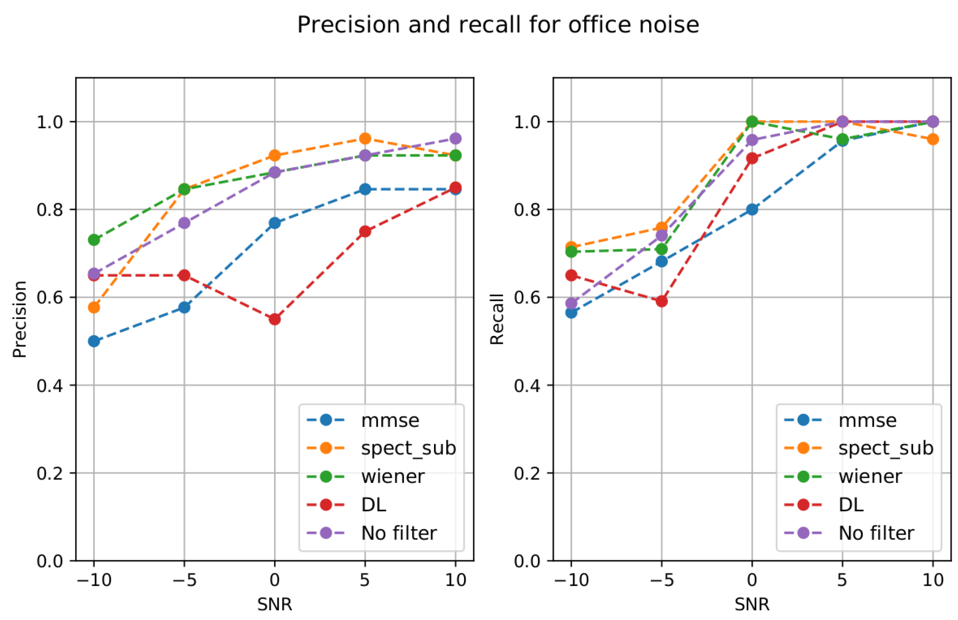
The mixed benefits of the different denoising algorithms are summarized in Figure 6. The deep learning was unable to successfully filter the Office noise in terms of the biometric identification. However, such results should be interpreted in the context of the amount of data available for the first stage of neural network training and the second stage of classification.

4. Discussion

The results presented in the Section 3 show how the different denoising algorithms differ in their capacity to enhance the sound signal for proper biometric identification of individuals. The main differences arose in the higher levels of noise (SNR −10 and SNR −5) for the two natural noises: Babble and Office.

The case of White noise seems to affect the biometric identification in a less considerable way across all SNR levels. This can be explained by the stationary nature of white noise, compared to natural noises like Babble and Office.

Given that each of the audio segments of the dataset has a length of five seconds, the sound of the footsteps may occur at any point in the audio. This means that the impulsive nature of Office sound and the non-stationary nature of Babble can affect the audio in very different ways, thus producing training and testing sets that can be very difficult to identify for the algorithms.

For a similar reason, the corresponding algorithms may encounter a significant challenge in denoising signals degraded by natural noises, which explains the lower Accuracy, Precision, Recall, and F1-score presented for those cases.

The comparison of the denoising algorithms in terms of their advantages and disadvantages is presented in Table 16.

Table 16. Denoising algorithm comparison.

Algorithm	Advantages	Disadvantages
MMSE [24]	competitive results in the lower levels of noise (SNR 10)	The algorithm did not achieve good results in four of the five SNR levels for all kinds of noise
Spectral subtraction [25]	Easy of implementation. Achieved very good results for natural noises.	In the presence of White noise, the algorithm degrades the signals and significantly lower the accuracy and precision.
Wiener [27]	Obtains the best accuracy results of Babble noise, and competitive results for White noise.	A tendency to lower the accuracy for low levels of noise (SNR 10) was observed.
Deep learning [28]	Obtained the best performance in all SNR levels of White Noise.	Large training time. It may require much larger datasets to enhance natural noises.

Table 16. Denoising algorithm comparison.

Algorithm	Advantages	Disadvantages
MMSE [24]	competitive results in the lower levels of noise (SNR 10)	The algorithm did not achieve good results in four of the five SNR levels for all kinds of noise
Spectral subtraction [25]	Easy of implementation. Achieved very good results for natural noises.	In the presence of White noise, the algorithm degrades the signals and significantly lower the accuracy and precision.
Wiener [27]	Obtains the best accuracy results of Babble noise, and competitive results for White noise.	A tendency to lower the accuracy for low levels of noise (SNR 10) was observed.
Deep learning [28]	Obtained the best performance in all SNR levels of White Noise.	Large training time. It may require much larger datasets to enhance natural noises.

The results presented in this paper can be comparable to recent works in the literature. For example, in [29], an accuracy of 0.95 was achieved in a person’s identification, a similar value to our experiments at the lower levels of noise. The same metric can be compared to other works, like [30] (accuracy of 0.975) and more recently in [10] (accuracy of 0.98 using Convolutional Neural Networks).

Other than accuracy, the results are difficult to compare to other recent works on biometrics of footstep sounds given the dissimilarities between the datasets, and the focus on noisy environments of our study. The best algorithms for the classification of the state-of-the-art works may be tested in a similar way to our proposal, with several types of noise at several SNR levels, in order to bring the biometric identification closer to real-life environments.

5. Conclusions

In this investigation, a comparative analysis of the benefits of denoising algorithms for footstep sounds as biometrics was presented. The novelty of the study for the state-of-the-art work is its focus on considering noise as an unavoidable part of the real-life implementations of footstep sounds as biometrics.

Given the number of possibilities that a person’s identification can mean in terms of experimentation, for this study we focused on the simple case of binary classification using segments of five seconds of distant recording and decided on the SVM algorithm to identify the volunteers from the sound of their footsteps.

For the testing of the denoising algorithms, we chose three noise types and five noise levels. Such a large number of possibilities allow for the comparison of diverse scenarios and provide a baseline for the use of distant sound recognition of footsteps as a biometric under noisy conditions. The accuracy of the different conditions contemplated in the experiments presented a range of 0.60 to 1.0, where the lower values were obtained with the Office noise at SNR −10, and the higher with White Noise at SNR 10. After applying the denoising algorithms, the accuracy range is 0.71 to 1.0, but the filtering method should be properly chosen for each case.

For the real-life application of a biometric system using distant footstep sounds, the results allow us to foresee the possibility of adequate recognition performance when non-stationary noise levels are not too high and provide a basis for establishing when denoising filters are recommendable or not.

For example, when stationary White Gaussian noise is present, the deep learning denoising provides the best results, but none of the algorithms tested in the work seems to benefit the process for low levels of natural noise. Certainly, deep learning denoising has several other possibilities than those presented in this work. For example, taking advantage of transfer learning, or training networks to simultaneously denoise several types of noise can be considered in the future.

Another possibility is the application of two stages of deep learning for denoising and classification. This is a promising opportunity for the development of future systems, and is scalable in other cases, such as multiple class identification, or identification of a single person within a group. For any of those possibilities, the large amount of data required should be considered: and will probably need very controlled conditions during recording sessions to homogenize the recordings.

Future work may also include the comparison of feature selection for classification and the selection and weighting methods of the DCT coefficient that are part of the features employed in this research. The feature selection methods should also be analyzed in terms of their robustness for noisy environments using this research as a comparison baseline in order to evaluate possible performance improvement.

References

1. Down, M.P.; Sands, R.J. Biometrics: An overview of the technology, challenges and control considerations. Inf. Syst. Control. J. 2004, 4, 53–56. [Google Scholar]
2. AbdElaziz, A.A. A survey of smartphone-based Face Recognition systems for Security Purposes. Kafrelsheikh J. Inf. Sci. 2021, 2, 1–7. [Google Scholar] [CrossRef]
3. Vera-Rodriguez, R.; Lewis, R.P.; Mason, J.; Evans, N. Footstep recognition for a smart home environment. Int. J. Smart Home 2008, 2, 95–110. [Google Scholar]
4. Alsaadi, I.M. Study On Most Popular Behavioral Biometrics, Advantages, Disadvantages and Recent Applications: A Review. Int. J. Sci. Technol. Res. 2021, 10, 15–21. [Google Scholar]
5. Thomas, P.A.; Mathew, K.P. A broad review on non-intrusive active user authentication in biometrics. J. Ambient. Intell. Humaniz. Comput. 2021, 1–22, online ahead of print. [Google Scholar]
6. Gomez-Alanis, A.; Gonzalez-Lopez, J.A.; Peinado, A.M. GANBA: Generative Adversarial Network for Biometric Anti-Spoofing. Appl. Sci. 2022, 12, 1454. [Google Scholar] [CrossRef]
7. Pedotti, A. Simple equipment used in clinical practice for evaluation of locomotion. IEEE Trans. Biomed. Eng. 1977, 5, 456–461. [Google Scholar] [CrossRef] [PubMed]
8. Addlesee, M.D.; Jones, A.L.; Livesey, F.; Samaria, F. The ORL active floor [sensor system]. IEEE Pers. Commun. 1997, 4, 35–41. [Google Scholar] [CrossRef]
9. Rodriguez, R.V.; Evans, N.W.D.; Lewis, R.P.; Fauve, B.; Mason, J.S.D. An experimental study on the feasibility of footsteps as a biometric. In Proceedings of the 2007 15th European Signal Processing Conference, Poznan, Poland, 3–7 September 2007. [Google Scholar]
10. Algermissen, S.; Hörnlein, M. Person Identification by Footstep Sound Using Convolutional Neural Networks. Appl. Mech. 2021, 2, 257–273. [Google Scholar] [CrossRef]
11. Hori, Y.; Ando, T.; Fukuda, A. Personal Identification Methods Using Footsteps of One Step. In Proceedings of the 2020 International Conference on Artificial Intelligence in Information and Communication (ICAIIC), Fukuoka, Japan, 19–21 February 2020. [Google Scholar]
12. Mason, J.E.; Traoré, I.; Woungang, I. Gait Biometric Recognition. In Machine Learning Techniques for Gait Biometric Recognition; Springer: Cham, Switzerland, 2016; pp. 9–35. [Google Scholar]
13. Connor, P.; Ross, A. Biometric recognition by gait: A survey of modalities and features. Comput. Vis. Image Underst. 2018, 167, 1–27. [Google Scholar] [CrossRef]
14. Vera-Rodriguez, R.; Mason, J.S.D.; Ortega-Garcia, J.F.J. Analysis of time domain information for footstep recognition. In International Symposium on Visual Computing; Springer: Berlin/Heidelberg, Germany, 2010. [Google Scholar]
15. Shoji, Y.; Takasuka, T.; Yasukawa, H. Personal identification using footstep detection. In Proceedings of the 2004 International Symposium on Intelligent Signal Processing and Communication Systems, ISPACS 2004, Seoul, Korea, 18–19 November 2004. [Google Scholar]
16. Tsuji, K.; Takao, R.; Yamada, M.; Harada, K.; Kamiya, Y. Multiple Person Detection by Footsteps Sounds Using GMRS. IEEE Sens. J. 2020, 21, 6543–6554. [Google Scholar] [CrossRef]
17. Naqvi, S.Z.H.; Choudhry, M.A. An automated system for classification of chronic obstructive pulmonary disease and pneumonia patients using lung sound analysis. Sensors 2020, 20, 6512. [Google Scholar] [CrossRef]
18. García-Domínguez, A.; Galván-Tejada, C.E.; Brena, R.F.; Aguileta, A.A.; Galván-Tejada, J.I.; Gamboa-Rosales, H.; Celaya-Padilla, J.M.; Luna-García, H. Children’s Activity Classification for Domestic Risk Scenarios Using Environmental Sound and a Bayesian Network. Healthcare 2021, 9, 884. [Google Scholar] [CrossRef] [PubMed]
19. Leng, L.; Li, M.; Kim, C.; Bi, X. Dual-source discrimination power analysis for multi-instance contactless palmprint recognition. Multimed. Tools Appl. 2017, 76, 333–354. [Google Scholar] [CrossRef]
20. Giannakopoulos, T. Pyaudioanalysis: An open-source python library for audio signal analysis. PLoS ONE 2015, 10, e0144610. [Google Scholar] [CrossRef]
21. Bachu, R.G.; Adapa, B.K.; Kopparthi, S.; Buket, D. Barkana Separation of voiced and unvoiced using zero crossing rate and energy of the speech signal. In Proceedings of the American Society for Engineering Education (ASEE) Zone Conference Proceedings, Pittsburgh, PA, USA, 22–25 June 2008. [Google Scholar]
22. Acharya, U.R.; Fujitad, H.; Sudarshan, V.K.; Bhate, S.; Koh, J.E.W. Application of entropies for automated diagnosis of epilepsy using EEG signals: A review. Knowl.-Based Syst. 2015, 88, 85–96. [Google Scholar] [CrossRef]
23. Tiwari, V. MFCC and its applications in speaker recognition. Int. J. Emerg. Technol. 2010, 1, 19–22. [Google Scholar]
24. Yu, D.; Deng, L.; Droppo, J.; Wu, J.; Gong, Y.; Acero, A. A minimum-mean-square-error noise reduction algorithm on mel-frequency cepstra for robust speech recognition. In Proceedings of the 2008 IEEE International Conference on Acoustics, Speech and Signal Processing, Las Vegas, NV, USA, 31 March–4 April 2008. [Google Scholar]
25. Kamath, S.; Loizou, P. A multi-band spectral subtraction method for enhancing speech corrupted by colored noise. In Proceedings of the 2002 IEEE International Conference on Acoustics, Speech, and Signal Processing, Orlando, FL, USA, 13–17 May 2002; Volume 4. [Google Scholar]
26. El-Fattah, M.A.A.; Dessouky, M.I.; Abbas, A.M.; Diab, S.M.; El-Rabaie, E.L.M.; Al-Nuaimy, W.; Alshebeili, S.A.; El-samie, F.E.A. Speech enhancement with an adaptive Wiener filter. Int. J. Speech Technol. 2014, 17, 53–64. [Google Scholar] [CrossRef]
27. Upadhyay, N.; Jaiswal, R.K. Single channel speech enhancement: Using Wiener filtering with recursive noise estimation. Proc. Comput. Sci. 2016, 84, 22–30. [Google Scholar] [CrossRef]
28. Defossez, A.; Synnaeve, G.; Adi, Y. Real time speech enhancement in the waveform domain. arXiv 2020, arXiv:2006.12847. [Google Scholar]
29. Altaf, M.U.B.; Butko, T.; Juang, B.-H. Person identification using biometric markers from footsteps sound. In Proceedings of the INTERSPEECH, Lyon, France, 25–29 August 2013. [Google Scholar]
30. Riwurohi, J.E.; Riwurohi, J.E.; Mustofa, K. Agfianto Eko Putra People recognition through footstep sound using MFCC extraction method of artificial neural network back propagation. Int. J. Comput. Sci. Netw. Secur. 2018, 18, 28–35. [Google Scholar]
Figure 1. Illustration of the recording session.
Computation 10 00133 g001
Figure 2. Sample waveform and spectrogram of a segment of five seconds from the first volunteer, during several stages of the experimental process. (a) Clean segment. (b) Noise-degraded with White Noise SNR 0. (c) After the deep-learning based denoising.
Computation 10 00133 g002aComputation 10 00133 g002b
Figure 3. Sample waveform and spectrogram of a segment of five seconds from the first volunteer, during several stages of the experimental process. (a) Clean segment. (b) Noise-degraded with Office Noise SNR 0. (c) After the deep learning-based denoising.
Computation 10 00133 g003
Figure 4. Comparison of Precision and Recall results for Babble.
Computation 10 00133 g004
Figure 5. Comparison of Precision and Recall results for White noise.
Computation 10 00133 g005
Figure 6. Comparison of Precision and Recall results for Office noise.
Computation 10 00133 g006
Publisher’s Note: MDPI stays neutral with regard to jurisdictional claims in published maps and institutional affiliations.