Article

A Multiobjective Variable Neighborhood Strategy Adaptive Search to Optimize the Dynamic EMS Location–Allocation Problem

by
Ponglert Sangkaphet
1,
Rapeepan Pitakaso
2,
Kanchana Sethanan
3,
Natthapong Nanthasamroeng
4,
Kiatisak Pranet
5,
Surajet Khonjun
2,
Thanatkij Srichok
2,
Sasitorn Kaewman
6 and
Chutchai Kaewta
7,*
1
Artificial Intelligence Optimization SMART Laboratory, Department of Computer Science, Faculty of Computer Science, Ubon Ratchathani Rajabhat University, Ubon Ratchathani 34000, Thailand
2
Artificial Intelligence Optimization SMART Laboratory, Department of Industrial Engineering, Faculty of Engineering, Ubon Ratchathani University, Ubon Ratchathani 34190, Thailand
3
Research Unit on System Modeling for Industry, Department of Industrial Engineering, Faculty of Engineering, Khon Kaen University, Khon Kaen 40002, Thailand
4
Artificial Intelligence Optimization SMART Laboratory, Department of Engineering Technology, Faculty of Industrial Technology, Ubon Ratchathani Rajabhat University, Ubon Ratchathani 34000, Thailand
5
Artificial Intelligence Optimization SMART Laboratory, Department of Logistics Management, Faculty of Industrial Technology, Ubon Ratchathani Rajabhat University, Ubon Ratchathani 34000, Thailand
6
Department of Computer Science, Faculty of Informatics, Mahasarakham University, Mahasarakham 44000, Thailand
7
Artificial Intelligence Optimization SMART Laboratory, Department of Digital Innovation, Faculty of Computer Science, Ubon Ratchathani Rajabhat University, Ubon Ratchathani 34000, Thailand
*
Author to whom correspondence should be addressed.
Computation 2022, 10(6), 103; https://doi.org/10.3390/computation10060103
Submission received: 17 May 2022 / Revised: 11 June 2022 / Accepted: 15 June 2022 / Published: 20 June 2022

Abstract

:
An aging society increases the demand for emergency services, such as EMS. The more often EMS is needed by patients, the more medical staff are needed. During the COVID-19 pandemic, the lack of medical staff became a critical issue. This research aims to combine the allocation of trained volunteers to substitute for medical staff and solve the EMS relocation problem. The objective of the proposed research is to (1) minimize the costs of the system and (2) maximize the number of people covered by the EMS within a predefined time. A multiobjective variable neighborhood strategy adaptive search (M-VaNSAS) has been developed to solve the problem. From the computational results, it can be seen that the proposed method obtained a better solution than that of current practice and the genetic algorithm by 32.06% and 13.43%, respectively.

1. Introduction

1.1. Motivation

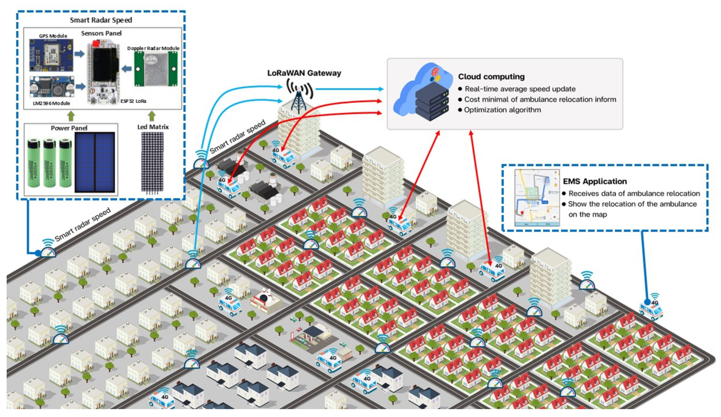
The International Social Security Association (ISSA) reports that the proportion of the population over 64 years old will increase from 16% to 26% by 2050. The aging of the world’s population is accelerating. The larger size of the aging population confirms the development of the world’s healthcare system; however, it also requires reformulating various public policies such as health, housing, social services, and pension systems. Elderly people prefer to remain in their own homes rather than moving into retirement care facilities; thus, older people inhabit homes that are randomly spread throughout a city. When an emergency service is needed due to a health problem of an elderly person, the emergency medical service (EMS) needs to arrive at the target location within a predefined time in order to, potentially, save the life of the patient. The traveling time of the EMS to the patient depends on (1) the distance from the EMS’s location to the patient’s location and (2) the current traffic situation (CTS) of the route used by the EMS. Sometimes, even when the EMS is located close to the patient’s location, the traveling time is high due to current traffic conditions. This paper presents a methodology to solve the EMS’s location problem (EMS-LP), and the current traffic situation is considered. A multiobjective variable neighborhood strategy adaptive search (M-VaNSAS) is used to solve the EMS-LP, while the IOT is used to track the CTS. The IOT sends the CTS to the central processing unit (CPU); then, the M-VaNSAS uses these data to calculate the correct location of the EMS. A correct location of the EMS is defined as enabling the EMS to arrive at the patient’s location within a predefined time. The predefined time is divided into two categories: (1) promised service time (PST: R2); (2) excellent service time (EST: R1). R1 is set to 8 min, and R2 is set to 20 min. As the number of elderly people is growing, the number of required EMSs is also increasing. EMS cars/trucks (hardware) are not difficult to find or buy for use in the healthcare system; however, the number of emergency medical technicians (EMTs), who need to be on standby with the EMS, is always limited. In Thailand, trained volunteers (TVs) are used as substitutes for experienced EMTs. Different TVs have different experience levels and different costs. The experience of the EMT affects the chances of the survival of the patient in severe cases. An EMS needs enough experienced staff in order to guarantee the service quality of all EMSs in the system; thus, the assignment of the right TV to an EMS offers the full capability of the EMS to rescue patients before sending them to the hospital. In this study, the assignment of TVs to work with the EMS is integrated into the model; therefore, the EMS has full capacity and the lowest assignment cost. In this article, we present a combination of the EMS relocation problem and the TV assignment problem (EMS-LP-TVS) in order to maximize the following objectives: (1) minimize the total costs of the system; (2) maximize the number of people who can be covered within the R1 time. The framework of the proposed problem is shown in Figure 1.
Figure 1 illustrates the proposed problem and an approach to finding a solution. It begins with installing equipment to assess the current traffic situation (smart radar speed); information from this IOT device is sent via LoRa over the internet to the server; then, the server sends information back to the EMS and TV via a mobile application. In this step, the staff assignment and EMS relocation algorithm are used.

1.2. Related Works

The EMS location/relocation (EMS-L/R) problem is to locate/relocate the EMS whenever the traffic situation or patient demand is changed. The EMS-L/R has been solved statically [1,2,3] and dynamically [4]. Static planning deals with a single period; Zidi et al. [5] presented a mathematical model based on the vehicle routing problem to represent the EMS location problem and solved it by a hybrid simulated annealing algorithm and tabu search (SA-TS). The demand and traveling time were collected from historical data. When the result was obtained, it was used until the new demand and traveling time were obtained (the next planning period). Bélanger et al. [6] presented a combination of EMS static location planning with an EMS dispatching strategy to reach the patient within the specified time, while Mouhcine et al. [7] included road accident history in the model to create an optimal route for the EMS.
Researchers focus more on dynamic planning, where the location/relocation is determined through multiple period planning. Multiple period planning is needed due to the changing demand of the EMS and the fact that the traveling time from the current location to the patient may change during the time of the day or the day of the week. Schmid and Doerner [8] presented a mixed integer program to represent a multiperiod EMS location problem in which the current traffic situation was integrated into the model. The average speed of the traffic along a street, which varied depending on the time of day, was collected. These data were used to calculate the optimal location of the EMS, which varied throughout the day, and the result showed that the dynamic relocation strategies had better performance than the static ones. Rajagopalan et al. [9] presented a comprehensive simulation model to minimize the number of ambulances used to service the varying patient demand. This research also focused on multiple period planning in which the demand of the patients and traveling time of the EMS varied throughout the planning time. EMS demand varies with time, such as on a working day, when people are in office locations, while on the weekend, people may stay home or be in shopping areas; thus, the location of the population varies throughout time.
The traveling time of the EMS is affected by the current traffic situation of the city’s streets. Most research has used historical data, which were collected manually or electronically from the electronic devices. These electronic devices include speedometers, radar, and range finders. While these devices have been widely used by the police and researchers, they have not been used in the real-time relocation problem.
The critical issue mentioned during the COVID-19 pandemic [10] was healthcare system management, particularly the resource allocation problem. Ma et al. [11] proposed a dynamic programming model to study bed allocation in hospitals for different patient types during the pandemic. Yuk-Chiu Yip [12] presented guidelines for healthcare resource allocation based on an ethical analysis. Biswas et al. [13] revealed the composition of the COVID-19 exposure-measurement framework, which can help with vaccine prioritization and resource allocation. Kim et al. [14] showed that a vaccine with lower resource requirements (wider reach) can significantly contribute to reducing the infection rate of the population and revealed that the tradeoffs between efficacy and reach are critical for resource allocation decisions between different vaccine types for improving health outcomes. From the mentioned research, we can see that during the pandemic, resource availability was the critical issue to manage. Human resources in the healthcare system are one of the most critical parts that cannot be boosted in a very short time to cover a difficult period, such as the COVID-19 pandemic. Chen et al. [15] studied the problem by integrating medical staff allocation and the staff scheduling problem in uncertain environments using a two-stage algorithm based on goal programming to determine the smallest possible number of medical staff required and to create the best schedule for them. Vieira et al. [16] proposed a stochastic mixed-integer linear programming model that optimized the allocation of radiation therapy technologists to multiple operations in radiotherapy over a set of scenarios of patient inflow. The goal was to maximize the (expected) number of patients completing pretreatment within the waiting time target. An EMS requires a high number of medical staff since every minute the patient has to wait for medical treatment dramatically reduces their chance of survival. In Thailand, the EMS stands by at the location from which it can reach patients within the predefined time. However, a large city such as Ubon Ratchathani, Thailand, with more than 1.5 million inhabitants, needs a high number of EMSs. Each EMS vehicle needs at least two staff, one driver, and one medical staff member who can provide first aid to the patients. During the pandemic, medical staff needed to remain on standby at hospitals; therefore, they could not be on standby with the EMS at the EMS locations. Here, a medically trained volunteer (TV) could be used as a substitute for professional medical staff [17,18,19]. The TV has different experience, which results in different pay. Therefore, the right assignment of a TV to an EMS will generate a suitable cost for the city and the service quality of the EMS. In this research, the experiences of a TV will be collected and assigned to a specified EMS. All EMSs must have a minimum service quality, which is controlled by the minimum total experience level of the TV with the responsibility for a specified EMS.
The EMS-LP-TVS is the first time that staff allocation and EMS relocation problems have been integrated. Previously, the EMS relocation problem has been integrated with other NP-hard problems, such as the dispatching problem [6] and the vehicle routing problem [7,20,21,22,23]. The methodology used to solve the EMS and location/relocation problem has included set covering and its extension [24,25], tabu search [4], linear programming [26], variable neighborhood search (VNS) [8,27], hybridization of simulated annealing algorithm and tabu search [5,28], particle swarm optimization [29], and ant colony optimization [7].
The algorithm used in this research is the variable neighborhood strategies adaptive search (VaNSAS), which was first proposed by Pitakaso et al. [30], who used VaNSAS to solve the location routing problem. VaNSAS comprises four steps: (1) generate an initial set of tracks (solution); (2) perform the track touring process; (3) update the heuristics information; (4) repeat steps 2 and 3 until termination. The basic concept of VaNSAS is that the quality of the current solution improves by using many types of heuristics. The heuristics include metaheuristics, simple heuristics, or the well-known local search procedure. Generally, three to four heuristics are designed for use in VaNSAS. The track can be used to select the heuristics in black box optimization. A suitable improvement procedure (IP) is selected with different probabilities. The probability of selecting the IP is iteratively updated depending on the average solution quality of tracks that previously used that IP. VaNSAS has been successfully used to solve various problems, such as the location routing problem, assembly line balancing problem [31], and scheduling and routing problems [32].

1.3. Contribution

This study aims to find the procedure to assign the TVs to the EMSs and locate the EMSs at the right place, so that an EMS can reach the patient before the PST. The objectives of the proposed procedure are to (1) minimize the total costs of the system (traveling cost and TV assignment cost) and (2) maximize the number of people covered within R1. The multiobjective EMS location model has been developed to solve this problem. The objectives’ function is evaluated using (1) the weighted sum method and (2) Pareto front analysis. The contribution of our research is as follows.
  • The assignment of the trained medical volunteer (TV) is first integrated into the EMS location problem. Due to the limitation of medical staff during a pandemic, a shortage of medical staff occurs; hence, a TV is used as a substitute for the medical staff; however, the levels of TVs’ experience are different. If the TV’s assignment is not suitable, it can affect the ability of the EMS to rescue the patients, which is the main concern of this article.
  • The IOT is used to collect the real average speed of a car along a particular road obtained from speed checkpoints. The IOT’s device submits this information to the EMS center, the data are analyzed, and real-time location information is sent to the EMS. This can help the EMS to reach the patients within the PST.
  • A new black box (improvement box) selection formula is first presented to improve the search performance of the original VaNSAS. A multiobjective variable neighborhood strategy adaptive Search (M-VaNSAS) is presented in this paper, and it is evaluated in comparison to existing well-known metaheuristics.
This paper is organized as follows. Section 2 discusses the related work and background to this study. Section 3 presents the proposed method, which is a modified differential evolution algorithm, while Section 4 and Section 5 present the computational results and conclusions, respectively.

2. Mathematical Model Formulation

In this section, the mathematical model is developed for the proposed problem (EMS-LP-TVS).
  • Indices
    • i: EMS i (i = 1,2,3,…,I)
    • l: Trained volunteer (TV)
    • k = 1,2,3,…,K
    • j: Community j (j = 1,2,3,..,J)
    • t: Time period t (t = 1,2,3,..,T)
  • Parameters
    • I: Number of EMSs
    • J: Number of communities
    • H: Maximum traveling time from the EMS to the community
    • R1: EST time
    • R2: PST time
    • El: Experience level of TV l
    • F l 1       i f   TV   l   i s   h i g h l y   e x p e r i e n c e d   TV 0     o t h e r w i s e                                                                                        
    • Tijt: Traveling time per kilometer from i to j at time t (min)
    • L: Number of trained volunteers
    • T: Length of planning period
    • O: Maximum communities that an EMS can serve
    • M: Minimum level of experience in an EMS
    • Cl: Cost of TV l (THB)
    • D: Maximum number of TVs in one EMS
    • Ai: Capacity of EMS i
    • Pjt: Size of population in j time t
    • B: Traveling cost per min of an EMS
  • Decision Variables
    • X i j t     1   when   EMS   i   serve   community   j   at   time   t   0       otherwise                                                                                                                        
    • N i j t     1   when   EMS     i   serve   community   j   not   within   R 1   at   time   t   0       otherwise                                                                                                                                                                                
    • Y i       1     if   EMS   i   is   in   use 0     otherwise                                  
    • S l i   1       if   TV   l   is   assigned   to   EMS   i 0     otherwise                                                                            
    • U i j t     Traveling   time   of   EMS   i   to   comunity   j   at   time   t
  • Objective Functions
    • M i n       Z 1 = t = 1 T j = 1 J i = 1 I B T i j t X i j t + l = 1 L i = 1 i C l S l i and   M a x       Z 2 = t = 1 T j = 1 J i = 1 I P i t 1 N i j t
  • Subject To
    •                                    U i j t     H                                             i ,   j   i = 1 I   j = 1 J   ( t 1 .. T )
                                          U i j t     T i j t X i j t                                    i ,   j   i = 1 I   j = 1 J   t 1 .. T
                                        U i j t   R 1 + ( H R 1 N i j t ]             i ,   j   i = 1 I   j = 1 J t 1 .. T
          j = 1 J P j t X i j t   A i Y i                        i   i = 1 I   t 1 .. T
          j = 1 J X i j t     O                                i   i = 1 I   t 1 .. T
            i = 1 I X i j t     2                                j   j = 1 J   t 1 .. T
      i = 1 I S l i 1                                     l   l = 1 L            
      l = 1 L E l S l i M                                 i   i = 1 I            
      l = 1 L F l S l i 1                                 i   i = 1 I            
Equation (1) shows the objective functions of the proposed problem, which is composed of two objectives: (1) Z1 is used to find the minimum total cost of operating the EMS, i, plus the traveling cost from i to j, and the assignment cost of the TVs to the EMS, and (2) Z2 is used to reveal the maximum number of people who are served within the R1 time. The first term of the first objective is the total distance used to travel from the location of EMS to the community multiplied by the traveling cost per kilometer. The result of multiplying is the total traveling cost that can occur in the system. The second term of the first objective operating cost of the EMS, when the TV is assigned to the EMS, will incur a cost and the summation of all assigned TV costs if it is the total operating cost of all EMSs. The second objective has one term which is the total population that are covered within R1 time by at least two EMSs (R1-CoV). The cost term is calculated by multiplying the size of the population of a community i at time t by one minus the community sign or number (0 or 1). If the community sign is 1, it means that the community is not covered within R1 by at least two EMSs, although we will obtain the total size of the population that are covered by at least one EMS within R1 time.
Equations (2) and (3) are used to define the traveling time from EMS i to j. Equation (4) shows whether community i can be reached by R1 or R2. Equations (2)–(4) have to be used together in order to form the value of U i j t ,   which is the decision variable that informs the system about what is the traveling time from community j to EMS i at time t, and it forces the decision variable N i j t to be zero or one. Equations (5) and (6) ensure that an EMS does not serve more patients than its capacity. Equation (5) controls the number of people that a particular EMS needs to service, which has to be less than its limitation, and Equation (6) is used to control the total number of communities that needs to be less than the EMS’s limitation. Equation (7) determines that a single community must be covered by at least two EMSs. Equations (8)–(10) are used to control the assignment of EMTs; i must have at least 1 experienced EMT, and the total experience of an EMS must be above the minimum requirement.

3. The Proposed Method

In our research, we propose the multiobjective variable neighborhood strategy adaptive search (M-VaNSAS). M-VaNSAS comprises four steps: (1) generate a set of initial tracks (solution); (2) perform the track touring process by using black box operators (improvement box: IB); (3) update the heuristics information; (4) repeat steps (2) and (3) until termination. How we used M-VaNSAS to solve the proposed problem is explained below.

3.1. Generate the Initial Tracks

In this section, the NT (number of tracks) was randomly generated. Table 1 represents four tracks. Each track had a dimension of 1 × D, where D represents the number of available EMSs. As shown in Table 1, D was set to 5. The initial WP used in this paper was a real number, which was uniformly randomly generated between 0 and 1 using Equation (11).
Y i j 1 = U 0 , 1
where Y i j 1 is the value in track i, position j, at iteration 1. j is defined as the number of available EMSs, and i is the predefined number of tracks. Another two sets of tracks were also randomly generated in the first iteration, the set of best tracks (BT) and random tracks (RT).
B i j 1 = U 0 , 1
R i j 1 = U 0 , 1
where B i j t is the set of the best solution collected from the best solution found, from iterations one to iteration t; R i j t was randomly selected using the formula. The first B i j t and R i j t , which had to appear in the first iteration, were randomly generated using Equations (12) and (13), respectively. Equation (14) was used to update Y i j t . The value of Y i j in iteration t + 1 was equal to the value of Y i j in iteration t, which used a selected IB operator. Table 1 shows an example of the four randomly generated tracks.
Table 1 shows the value of the track elements. Track 1 comprised five elements, which had values of 0.77, 0.07, 0.82, 0.14, and 0.44, respectively. They represent the value of the elements used to decode the proposed problem’s solution. The decoding method is explained in the following section.
  • The Decoding Method
The decoding method was used to decode the values of the elements representing the solution to the proposed problem. The decoding method used in this article comprises three steps: (1) assign communities to an available EMS (at least two EMSs must attend to a community within a predefined time: R1 = 12 min, R2 = 20 min); (2) sort the value of the elements from lowest to highest (list A); (3) assign the unused EMSs to the first position of list A; (4) reassign communities to the remaining EMSs; and (5) repeat steps (3) and (4) until a feasible solution is found during the assignment. The decoding method procedure is described in the following steps.
Table 2 shows the distance between the candidate location, the EMS, and the community (V) where the patients live.
Step 1: Assign the community to an available EMS. The results of Step 1 are shown in Table 3.
Communities 1 to 9 have the following numbers of inhabitants at time t: 100, 120, 220, 130, 150, 100, 140, 130, and 159 people, respectively, while the EMSs 1 to 5 have the capacities of 900, 800, 1000, 900, and 800, respectively. The limitation of the number of communities that an ambulance can cover is seven. The results of the first assignment are shown in Table 3.
Step 2: Sort the elements of value from lowest to highest. The sorting of track 1 is shown in Table 4.
From Table 4, the original track of track 1 value in element 1, 2, 3, 4, and 5 is 0.77, 0.07, 0.82, 0.14, and 0.77, respectively. The element will be sorted according to its value in elements in ascending order; thus, the new element sequence after the sorting is 2, 4, 5, 1, and 3, which have values in elements of 0.07, 0.14, 0.77, 0.77, and 0.82, respectively. The element sequence will be used in the next step of the proposed decoding method.
Step 3, Step 4, and Step 5 are performed simultaneously. The final result is shown in Table 5.
As seen in Table 5, EMS numbers 2 and 5 were unused, and the communities attended to by these two EMSs were assigned to other available EMSs. In relocating an EMS to the community, the following conditions must be considered: (1) the number of patients attended to by the EMS must be under the EMS’s capacity and (2) it must also be under the maximum number of communities the EMS can cover. In the next step, after we have obtained the used and unused EMSs, we will assign the TVs to the used EMSs. The methodology to assign the TVs to the used EMSs can be explained stepwise as follows.
  • Trained Volunteer Assignment Procedure
Step 1: Divide the TVs into two groups, which are experienced (El ≥ 1) and inexperienced (El < 1) TVs according to their predefined labor cost.
Step 2: For each group, sort the value of Cl in ascending order to obtain the lists of experienced TVs (List 1) and inexperienced TVs (List 2).
Step 3: Assign the first TV in List 1 to the first used EMS, and assign the second TV from the top of List 2; if the total experience level does not reach M, assign the second TV from the next position in List 2.
Step 4: Repeat Step 3 until all used EMSs are fully assigned to TVs. An example result of TV assignments is shown in Table 6.
From Table 6, there are nine TVs (1 to 9), who have an experience level of 0.8, 1.3, 1.3, 0.7, 0.9, 1.4, 0.5, 1.6, and 0.7, respectively. The cost of the nine TVs is 250, 360, 320, 260, 280, 390, 400, 420, and 400, respectively. The expected experience level of a TV is 2.0. Therefore, EMS 1 is served by TVs number 3 and number 1, EMS number 3 is served by TVs number 6 and number 4, and EMS number 5 is served by TVs number 2 and number 5.

3.2. Perform Track Touring Process

The tracks iteratively tour the black box. The black box features solution improvement methods that are not limited to a local search. The black box (improvement box: IB) can include metaheuristics, heuristics, and simple local search. In our research, four black boxes were designed to use the following methods: random-transit (RT), best-transit (BT), inter-transit (IT), and scaling factor (SF). We used a roulette wheel selection for the track to select the preferred black box. The selection of the black box is controlled by Equation (14).
P b t = F N b t 1 + 1 F A b t 1 + K I b t 1 + ρ A b t 1 A t 1 b e s t b = 1 B F N b t 1 + 1 F A b t 1 + K I b t 1 + ρ A b t 1 A t 1 b e s t
where P b t is the probability of selecting the black box in iteration t; N b t 1 is the total number of tracks that selected a black box in the previous iterations; Abt−1 is the average objective value of all tracks that selected black box b in all previous iterations; A t 1 b e s t is the global best solution found before iteration t; I b t 1 is a reward value, which increases by 1 if a black box finds the optimal solution in the last iteration but is set to 0 otherwise; B is the total number of black boxes; F is the scaling factor (F = 0.5); and K is the parameter factor (K = 1). Equation (14) is the formula that each track will select the preferred black box in each iteration. It is constructed based on four terms that can guide the solution to a good searching area. These terms are (1) number of times that the tracks have selected that black box in the previous iterations; (2) the average solution value of the tracks that have selected that black box; (3) if that black box contains the current best solutions; (4) how far the average solution of tracks that select that black box is from the solution of the best black box. We can see that, if the black box generates a good solution in previous iterations, it will increase the probability of selecting that black box in the current iteration.
The black box is operated using Formulas (15)–(18). Let us define the set of tracks in a single iteration. Assume that B is the number of tracks comprised in one iteration. Set A as the set of tracks that selected black box b, and set Z as the set of tracks that were not selected to operate in black box b, while the number of tracks in A plus Z is equal to B. We denote n as the track that was randomly chosen from the sets of track Z, and track i is the track that was chosen from the sets of track A.
      Random-transit   ( RT )      Y i j q = Y i j q 1           i f     R i j C   R i j q                   o t h e r w i s e        
  Best-transit   ( BT )      Y i j q = Y i j q 1           i f     R i j C B j g b e s t               o t h e r w i s e        
Inter-transit   ( IT )      Y i j q = Y i j q 1           i f     R i j C Y n j q                   o t h e r w i s e        
          Scaling   factor   ( SF )      Y i j q = Y i j q 1                     i f     R i j C   R i j Y i j q 1           o t h e r w i s e        
B j g b e s t and B h j p b e s t are the sets of tracks that gave the global best solution and best solution obtained from black box b, respectively. R i j is the random number of track i in position j.
Generally, the local search or local improvement of the metaheuristic is to increase two types of search capability: (1) diversification or exploration search; (2) intensification search. The exploration search behavior is designed to let the current solution escape from the local optimal solution and the intensification search will let the current solution search intensively for the current search space. Equations (15)–(18) fail in these two categories. Equations (15) and (18) are designed to increase the diversification or exploration capability, while Equations (16) and (17) are used to increase the intensification search. In Equation (16), the current solution is guided by the current best solution to the good searching space, while in Equation (17), the current solution is guided by the neighbor’s solution of it.
The sub-iteration update position of Y i j q + 1 was executed using Equation (19). q was the sub-iteration of black box b, which was the predefined parameter. C was the predefined parameter and was set to 0.7 [25]. The evaluation of the solution that was iteratively searched used Equation (20).
Y i j q + 1 = Y i j q           i f     f i t f i q       a n d   u p d a t e       f i t = f i q     a n d     Y i j t = Y i j q   Y r j q       o t h e r w i s e          
f i q = w 1 f i q 1 + w 2 f i q 2
where f i t is the objective function of track i at iteration t, and f i q is the objective function of track i at sub-iteration q. The objective used for Equation (20) derives from Equation (21), where w 1 is the random weight for objective 1, w 2 = (1 − w 1 ) , and w 1 =   U 0 , 1 . f i q 1 and f i q 2 are the objectives of objective Z1 and Z2, respectively.
M a x       Z = w 1 t = 1 T j = 1 J i = 1 I B T i j t X i j t + l = 1 L i = 1 i C l + w 2 t = 1 T j = 1 J i = 1 I P i t 1 N i j t
The Pareto front was used to retain the nondominated solution. We denote f 1 y r and f 2 y r as the objective functions of objective 1 and 2 of track r, respectively. Let R represent a set of feasible solutions, denote y = (y1,y2,…,yi), which is the set of decision vectors, and f v (y)=(   f 1 (y), f 2 (y),.., f V (y)) is the set of objective functions of vector y. y will dominate y’ if and only if f v (y) ≤ f v (y’) for all v = 1,2,3,…,V.
The promising solution from the Pareto front is analyzed using TOPSIS. The technique for order of preference by similarity to ideal solution (TOPSIS) is used to reveal the promising set of parameters. TOPSIS was first presented by Hwang and Yoon [33]. TOPSIS begins by constructing a normal decision matrix, which will transform various attributes’ dimensions into a non-dimensional attribute by using Equations (22)–(28).
r l v = x l v l = 1 L ( X l v ) 2
U l v = w v r l v
U v * = { max L U l v     i f     v V     ;   min L U l v       i f     v V * }
U v = {     min L U l v     i f     v V     ;   max L U l v       i f     v V }
S l * = v = 1 V ( U v * U l v ) 2
S l = v = 1 V ( U v U l v ) 2
C l * = S l S l * + S l
where x l v is the value of the objective function of point l objective v, l is the number of points in the Pareto front, V* is a set of positive objectives functions, and V’ is a set of negative objective functions. w v is the predefined parameter, which is the weight of each objective function. U* ( U * = U 1 * , U 2 * , ,   U n * ) and U’ ( U = U 1 , U 2 , ,   U n ) are the positive and negative ideal solutions, respectively. S l *   and S l   are the separation measures for each alternative from both the positive and negative ideal solutions, respectively, which will be used to calculate the relative closeness to the ideal solution ( C l * ) . The set of parameters that has a value of C l * closest to 1 will be selected as the promising solution.

3.3. Update the Probability of the Black Box (IB)

In this step, some of the heuristic information used in Equation (14) should be updated, and the variables to be updated are shown in Table 7.

3.4. Repeat Steps 3.2–3.3

Steps 3.2–3.3 are iteratively repeated until termination. The pseudocode of M-VaNSAS used in this paper is shown in Algorithm 1.
Algorithm 1: Multiobjective variable neighborhood strategy adaptive search (M-VaNSAS)-EMS
1
2
3
4
5
6
7
8
9
10
11
12
13
14
15
16
17
18
19
20
21
22
23
24
25
26
27
28
29
30
Input: Number of tracks (NT), Number of parameters (D), Scaling factor (F),
Improvement factor (K), Value of CR, Number of improvement box (IBPop)
Output: Best_Track_Solution
Begin
Population = Initialize Population (NT, D)
IBPop = Initialize InformationIB (NIB)
Encode Population to WP
while the stopping criterion is not met do
for i = 1: NT
//selected improvement box by roulette wheel selection
selected_IB = RouletteWheelSelection(IBPop)
if(selected_IB = 1) Then
new_u = RT (u)
Perform RT
else if(selected_IB = 2)
new_u = BT (u)
Perform BT
else if(selected_IB = 3)
new_u = IT (u)
Perform IT
else if(selected_IB = 4)
new_u = SF(u)
Perform SF
Perform Decoding method, Weight Sum Method
if(CostFunction(new_u) ≤ CostFunction(Vi)) Then
Vi = new_u
Update Pareto Front
End for loop //end update heuristics information
End while loop
End
As seen in Algorithm 1, M-VaNSAS will start by generating a set of initial solutions, known as the initial set of tracks. Then, this set of tracks will improve their solution quality by performing the improvement procedure using the black box. The black box will be used as a tool to improve the solution quality of the current set of tracks. There are four black box methods: RT, BT, IT, and SF. The tracks will iteratively search for the new solution. The maximum iteration of the searching of the tracks is the predefined variables, and it will be used as the stopping criterion for the proposed algorithm.

3.5. Comparison Methods

In this study, we compared the proposed methods using a genetic algorithm. A genetic algorithm (GA) is a nature-inspired metaheuristic that consists of four steps: (1) generate an initial solution; (2) perform a mutation procedure; (3) perform a crossover procedure; (4) perform a selection procedure. We modified the GA proposed by [34] for our problem. The selection process of GA was modified using Equation (21).

3.6. IOT and Mobile Application Architecture Design

Figure 2 shows the system architecture design, smart radar speed, which combines a battery power supply with solar cells, and was installed on a road to measure the speed of a car on that road. The Smart Radar Speed was connected to the LoRa network, which measures the speed of a car, obtains the coordinates from the GPS, and sends those data to the server to record the data in the database. Then, for every predefined planning period (t), the server calculates the average speed on each road to optimize the relocation of the ambulance. The server sends the updated information on the relocation of the ambulance to each ambulance via the EMS application for driving.
The design concept of this system consists of three main parts: smart radar speed, the EMS application, and the server system.
  • The smart radar speed consists of six components: an ESP32 LoRa, a GPS module, a Doppler radar module, an LM2596 module, a power panel, and an LED matrix. The Doppler radar module, GPS module, and LED matrix were connected to a printed circuit board; the core of the board is an ESP32 LoRa microcontroller, which has a 32-bit CPU operating at 160 MHz, with 16 MB of ROM and 512 KB of RAM, and the integrated LoRaWAN communication in the 920–925 MHz band [35]. The circuit board used the power from a 12 V lithium−ion rechargeable battery with a solar cell. The LM2596 module was used to generate 5 V of power for the circuit board. Furthermore, the LED matrix displays the car speed obtained from the Doppler radar module.
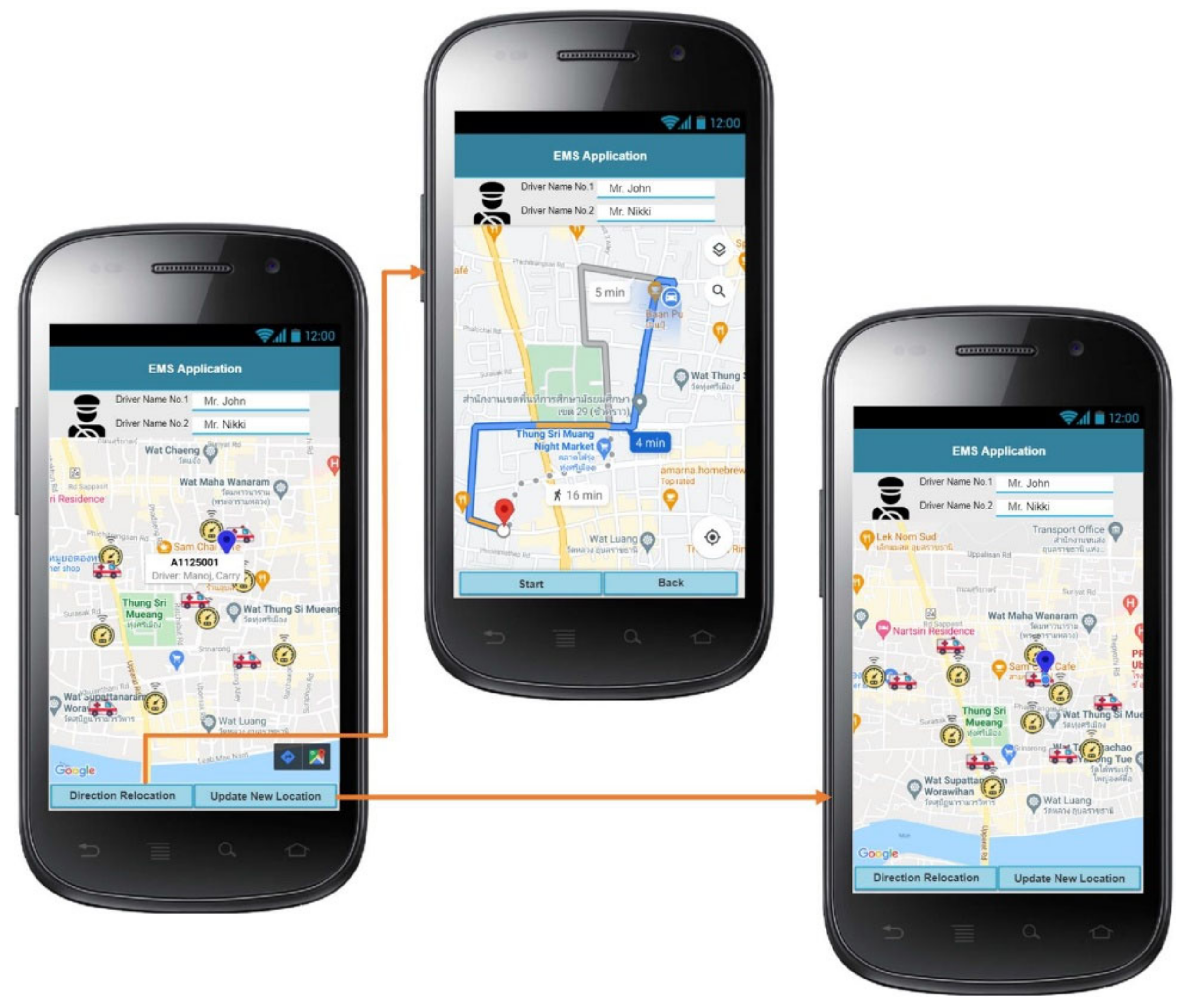
  • The EMS application, shown in Figure 3, runs on the Android platform. The EMS application needs to connect to 4G, with authentication via a login; then, the application obtains the data from the server’s database and displays them on the screen of the application. A Google Maps API displays the current location and journey of the ambulance on the application. Furthermore, the EMS application provides navigation when the system notifies the ambulance to relocate.
  • The server system performs the average speed calculation for each road and the lowest cost of the ambulance rerouting using an optimization algorithm; then, the server relays the ambulance relocation information to the EMS application.
In conclusion, the methodology to solve the proposed problem (EMS-LP-TVS), which is the combination of the EMS location problem and the trained medical volunteer (TV), is as follows.
(1)
Assign the TV to the EMS using M-VaNSAS algorithm.
(2)
Use current traffic condition to locate the EMS in the relevant location using M-VaNSAS algorithm.
(3)
Update real-time traffic situation using IOT and mobile application.
(4)
Reroute the EMS using M-VaNSAS algorithm.
(5)
Send the new location to the driver of EMS, leading back to step 1 (if needed).
(6)
Redo steps (3)–(5) at least every 3 h.
The proposed method was used as a tool for simulation and testing is reported in Section 4.

4. Computational Results and Framework

In this section, we divide the computational result into two parts: (1) the simulation result of the VaNSAS compared with GA using the randomly generated datasets; (2) the case study results compared with the current method.

4.1. Compare the Proposed Method (M-VaNSAS) with the Results from the Optimization Software (Lingo v.16) and the Genetic Algorithm

The proposed method was coded using Python and evaluated with a PC Intel ® Core ™ i5-2467M CPU 1.6 GHz, produced in USA. The testing of the performance of M-VaNSAS was on 14 randomly generated datasets compared with the existing heuristics. The details of the tests are shown in Table 8.
The details of the random parameters used to generate the tests are shown in Table 9.
In the first experiment, we used the GA and M-VaNSAS to solve the proposed problem for all 14 test instances. The GA and M-VaNSAS were used to collect the Pareto front; then, TOPSIS, with varying weights of w1 and w2, was used to evaluate the difference between both heuristics. The stopping criteria of GA and M-VaNSAS were set to 45 min for all test instances. Each instance was executed five times, and the best solution was used as representative of the method. Table 10 shows the computational results using various values of w1 and w2 (TOPSIS).
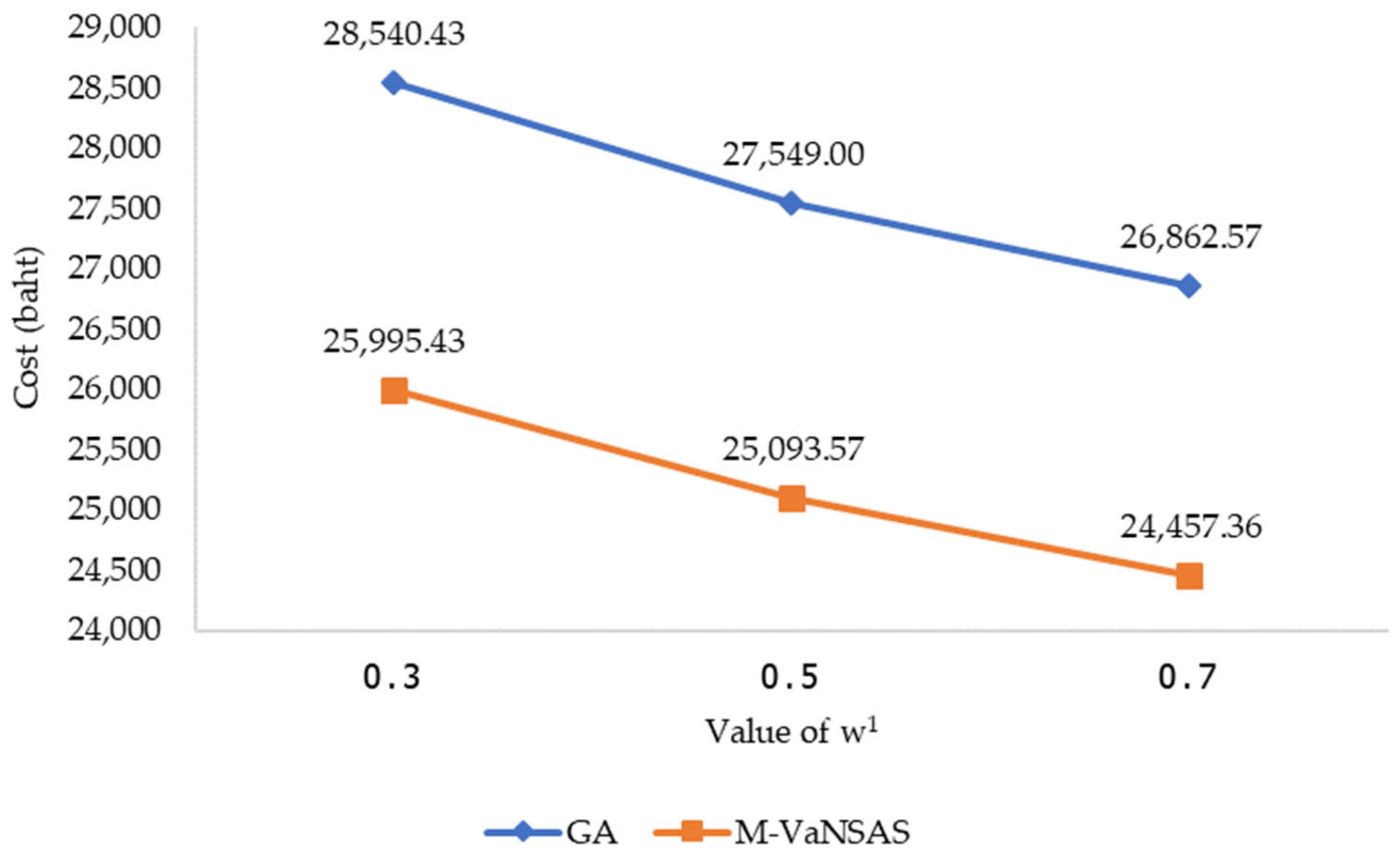
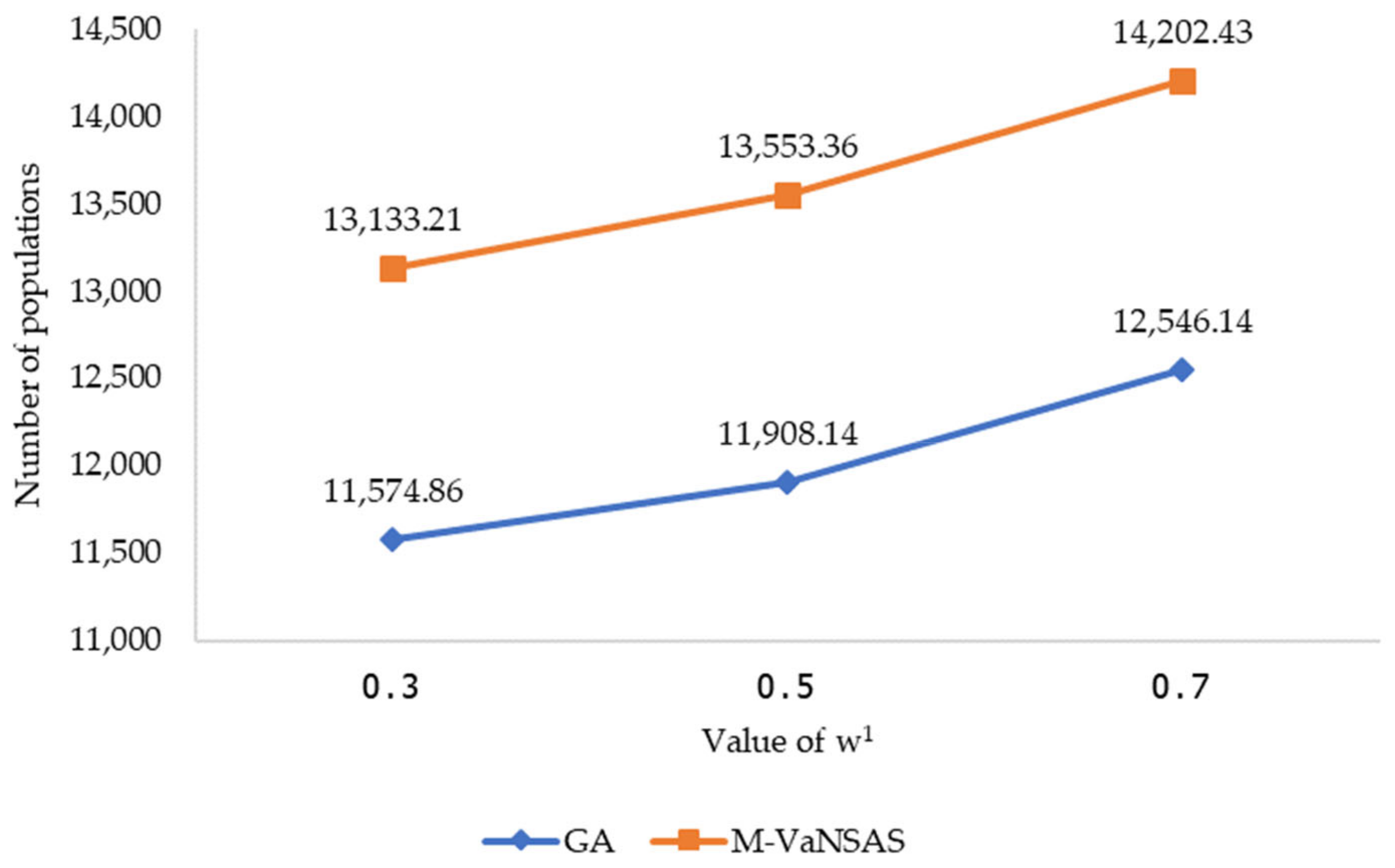
From Table 10, we can see that, on average, M-VaNSAS provided a better solution than that of GA. M-VaNSAS produced a 9.80% lower cost than that of GA and 13.49% more people were covered within the R1 time by the ambulance. Using the data obtained from Table 10, graphs plotted to show the effects of using different weights of w1 are presented in Figure 4 and Figure 5. The best objective for objective one (minimize total cost) is when we used M-VaNSAS with w1 = 0.7 and w2 = 0.3, while the best objective for the second objective (maximum population coverage) is when we used M-VaNSAS and set w1 = 0.3 and w2 = 0.7. On average, GA generated a worse solution than that of M-VaNSAS, at 14.25%. The relative difference (%diff) is calculated using Equation (29).
% d i f f = S C S B S B × 100 %
where S C is the candidate solution and S B is the best solution among all candidate solutions.
From Figure 4 and Figure 5, we can see that when the weight of w1 increased, the total cost of the system was lower, as w1 is the weight that focuses on reducing the total cost. In all w1 values, M-VaNSAS generated a lower cost than that of the GA. By contrast, when the weight of w1 increased, the Cov-R1 decreased, because an increase in w1 implies a decrease in the value of w2, which is the weight of increasing the Cov-R1 objectives.
The average ratio of the Pareto-optimal solution (ARP) was used to compare the performance of GA and M-VaNSAS in obtaining a good result for the proposed problem. Let N1,N2,…Nk be the number of iterations used in experiment k. n1, n2, …, nk are the number of Pareto-optimal solutions found in the kth experiment, and K is the total number of experiments. Therefore, the ARP is calculated using Equation (30).
A R P = n 1 N 1 + n 1 N 2 + + n k N k K
The results of the ARP are shown in Table 11.
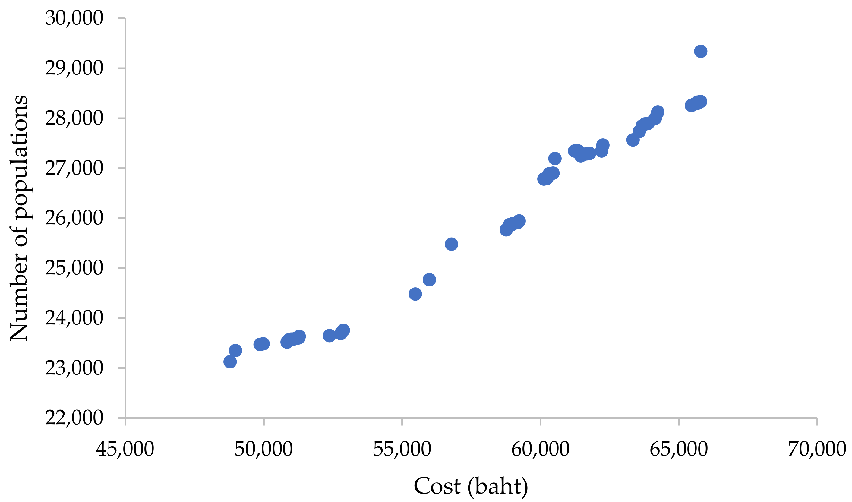
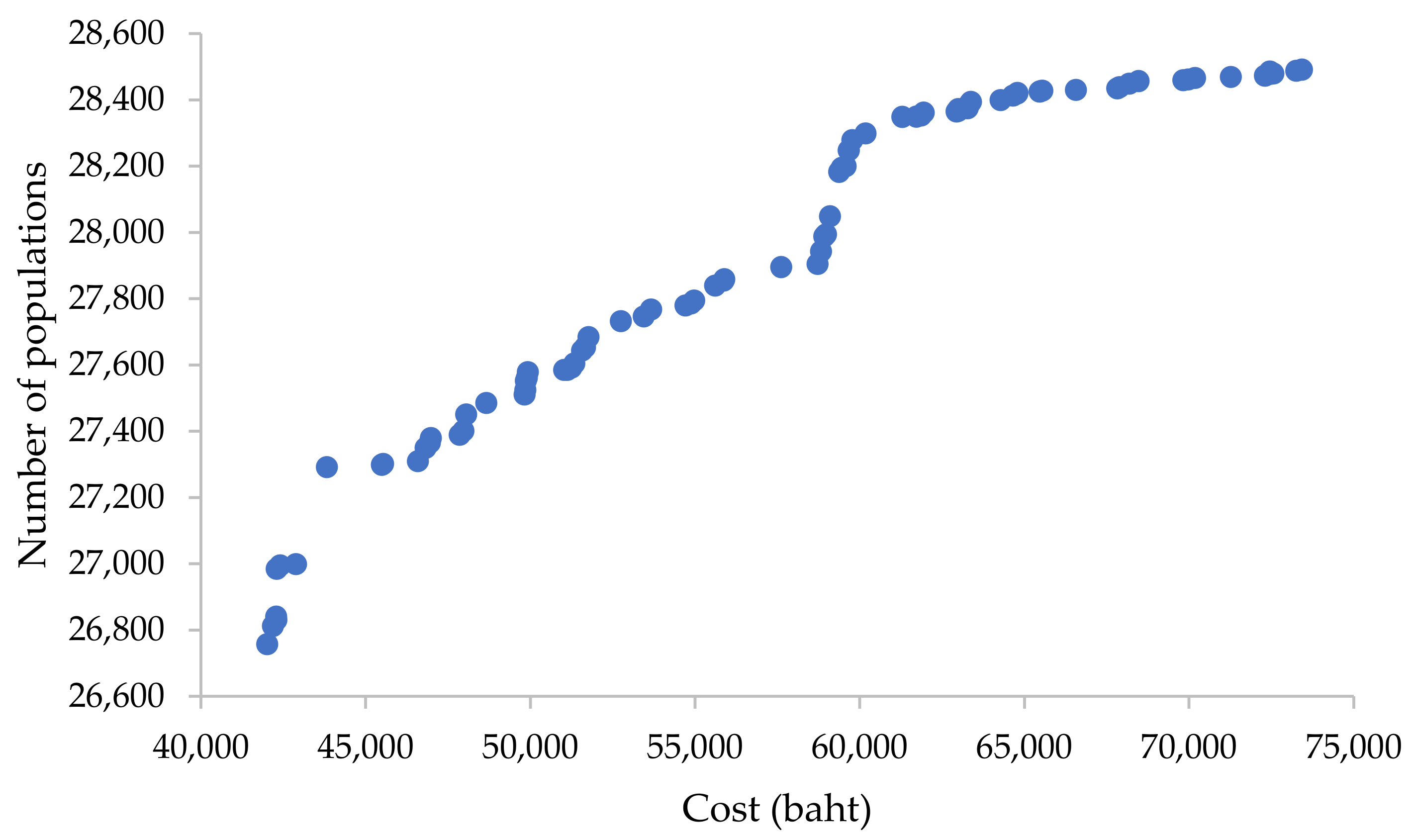
From the computational results shown in Table 11, we see that M-VaNSAS found 12.68% more Pareto points than the GA; thus, we can conclude that M-VaNSAS is better than the GA in finding more solutions. Figure 6 and Figure 7 compare the Pareto fronts of the M-VaNSAS and GA.
From Figure 6 and Figure 7, we can see that the Pareto front of the GA had more gaps between the Pareto points than that of M-VaNSAS. From the data that we collected, GA found 1680 Pareto points during 1500 iterations, while M-VaNSAS found 2014 points using the same number of iterations. The ARP of the GA was 16.42% less than that of M-VaNSAS, which means the chances of GA having a larger gap between each Pareto point were higher, as shown in Figure 6 and Figure 7.
The next experiment examined the effectiveness of the proposed method when we simplified the objective function of the proposed problem to see the cost expenditure per person. The objective function shown in Equation (1) was simplified to Equation (31). The solution was compared with the result obtained from Lingo V.16 within 480 h and the GA using 45 min of computational time. The results are shown in Table 12, and the statistical test using the Wilcoxon signed-rank test is shown in Table 13.
M i n       Z = t = 1 T j = 1 J i = 1 I B T i j t X i j t + l = 1 L i = 1 i C l S l i t = 1 T j = 1 J i = 1 I P i t 1 N i j t  
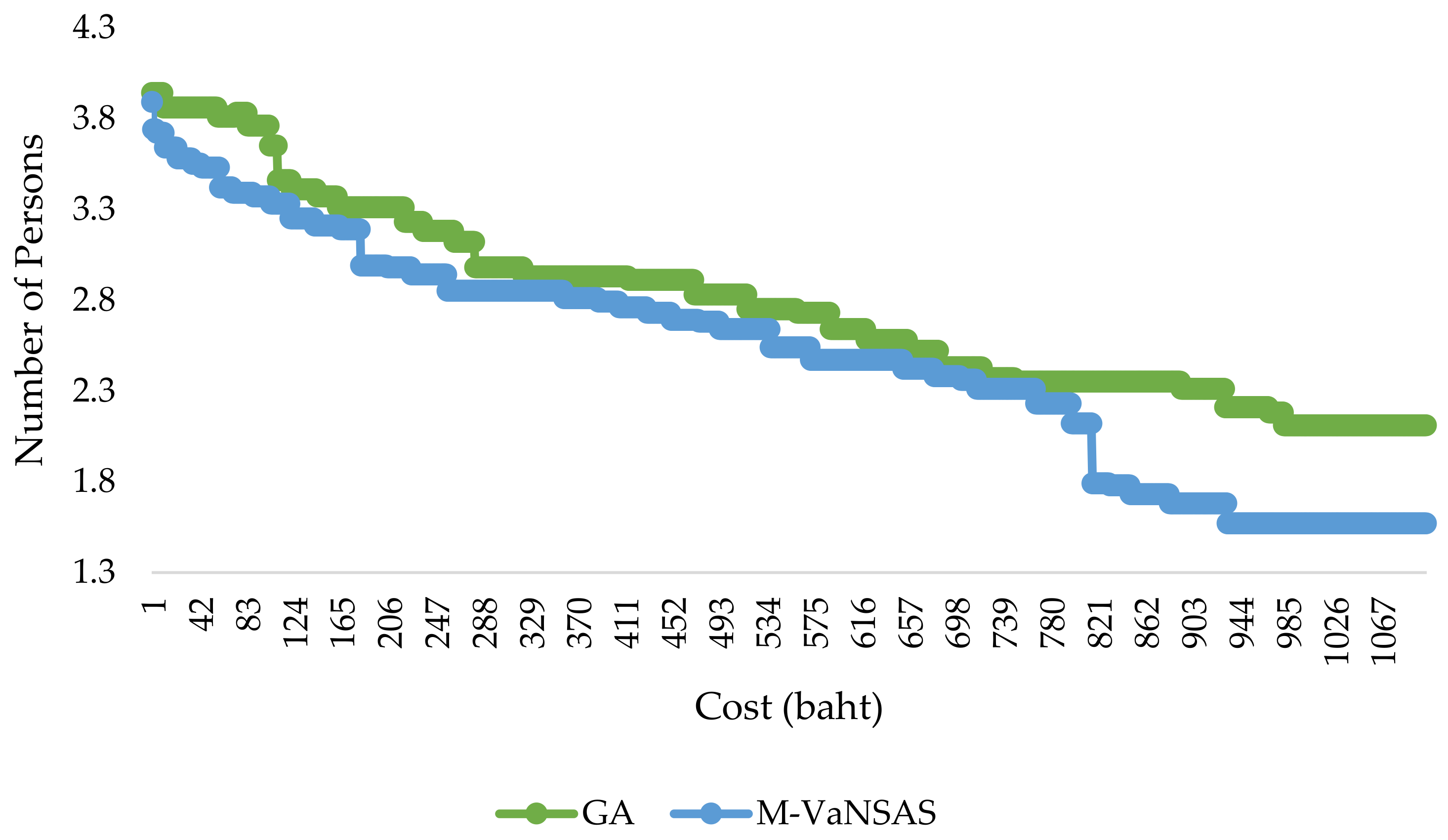
From Table 12 and Table 13, we can see that M-VaNSAS obtained the best result among all three methods. It significantly improved the solution obtained from the best result found by Lingo using 480 h by 44.15% and improved the solution quality of Lingo by 19.69%. Figure 8 shows the progressive plot of the best solutions found during 1100 iterations of the GA and M-VaNSAS.
From Figure 8, we can see that M-VaNSAS found a new solution during the search 132 times, while GA found a new best solution 101 times, which means that M-VaNSAS had a higher ability to find a good solution during the search; the average difference between the new best solution and the current best solution was 3.19%, while GA had an average difference of 1.87%. This implies that M-VaNSAS surpassed the local optimum more than the GA.
The next experiment we performed examined the efficiency of using a different black box or improvement box. In this experiment, Equation (31) was used as the objective function for all M-VaNSAS. The stopping criterion was the computational time, which was set to 45 min. All the proposed M-VaNSAS approaches were used to solve all 14 random test instances. Details of the subalgorithm of M-VaNSAS are shown in Table 14.
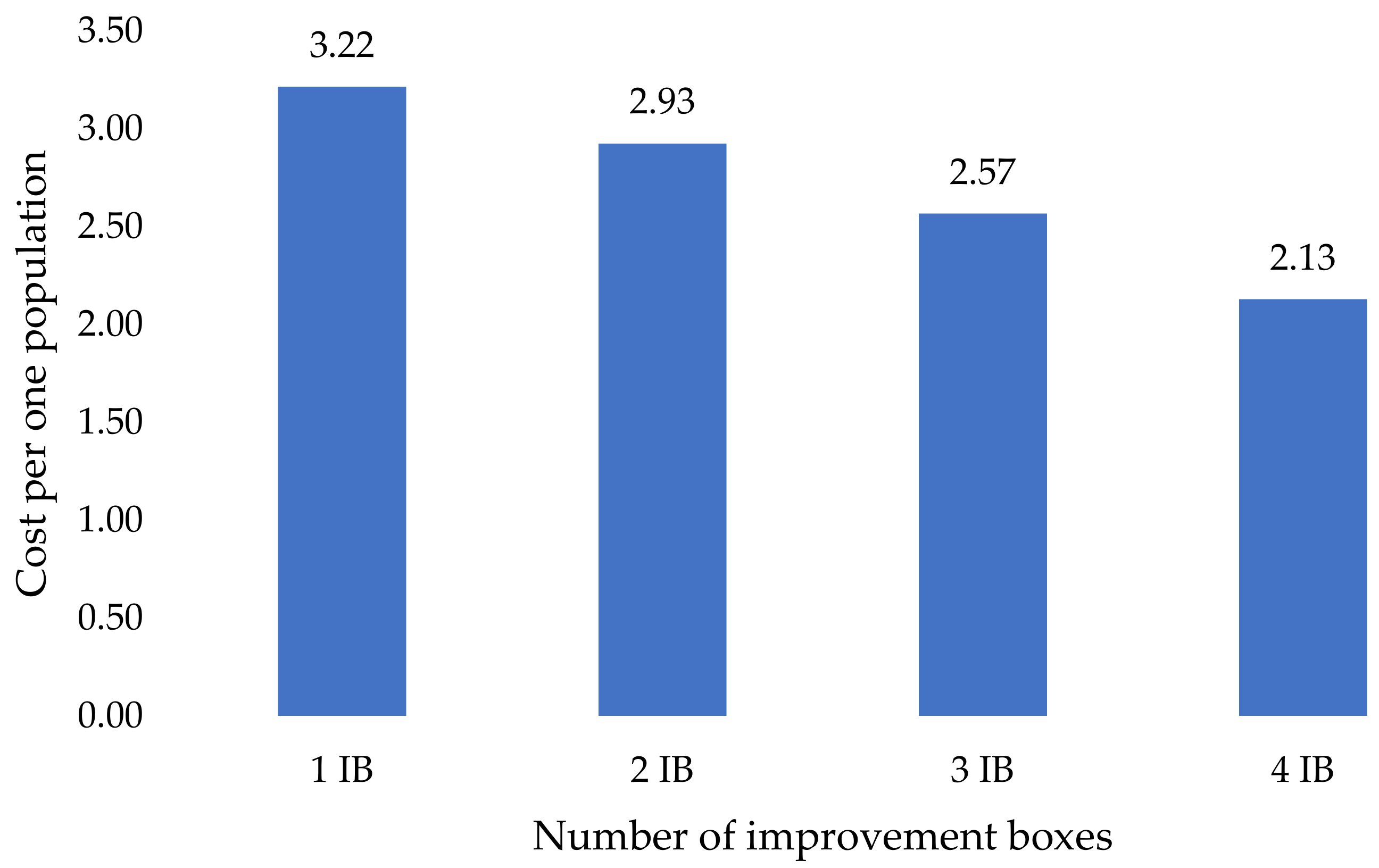
The checklist shown in Table 14 contains the improvement boxes used in the M-VaNSAS for each subalgorithm. The results of all the proposed M-VaNSAS approaches are shown in Table 15. The average cost used in different numbers of improvement boxes is shown in Figure 9.
From Table 15 and Figure 9, we can conclude that using 1 IB generated the highest cost, while using 4 IB generated the best solution among all the methods. M-VaNSAS-13, which used all the improvement boxes (four) in M-VaNSAS, obtained the best solution of all the methods. It obtained a lower cost than using 3, 2, and 1 IB by 33.76%, 27.21%, and 17.04%, respectively, with the same computational time. In sum, the use of a higher number of improvement boxes provided a better solution. In using the different relative results of the subalgorithms with the best subalgorithm, we found that 1, 2, and 3 IB exceeded the cost of 4 IB by 51.06%, 37.44%, and 20.54%, respectively.

4.2. Case Study Results Compared with the Current Method

The designed application and the M-VaNSAS were implemented in a real case study, the EMS service of Muang Ubon Ratchathani City, which has 217,396 people, 155 communities, and 35 EMS vans. M-VaNSAS was used for 30 days, and the results of the average arrival time at the patients, maximum and minimum arrival time at the patients, minimum total cost incurred during the 30 days, and the total distances covered by all EMSs were recorded. The results are shown in Table 15. GA was used for 30 days using the same real data obtained from the implementation of M-VaNSAS. The results of M-VaNSAS and GA were compared with current practice, which the city government uses to manage the EMS. The results are shown in Table 16.
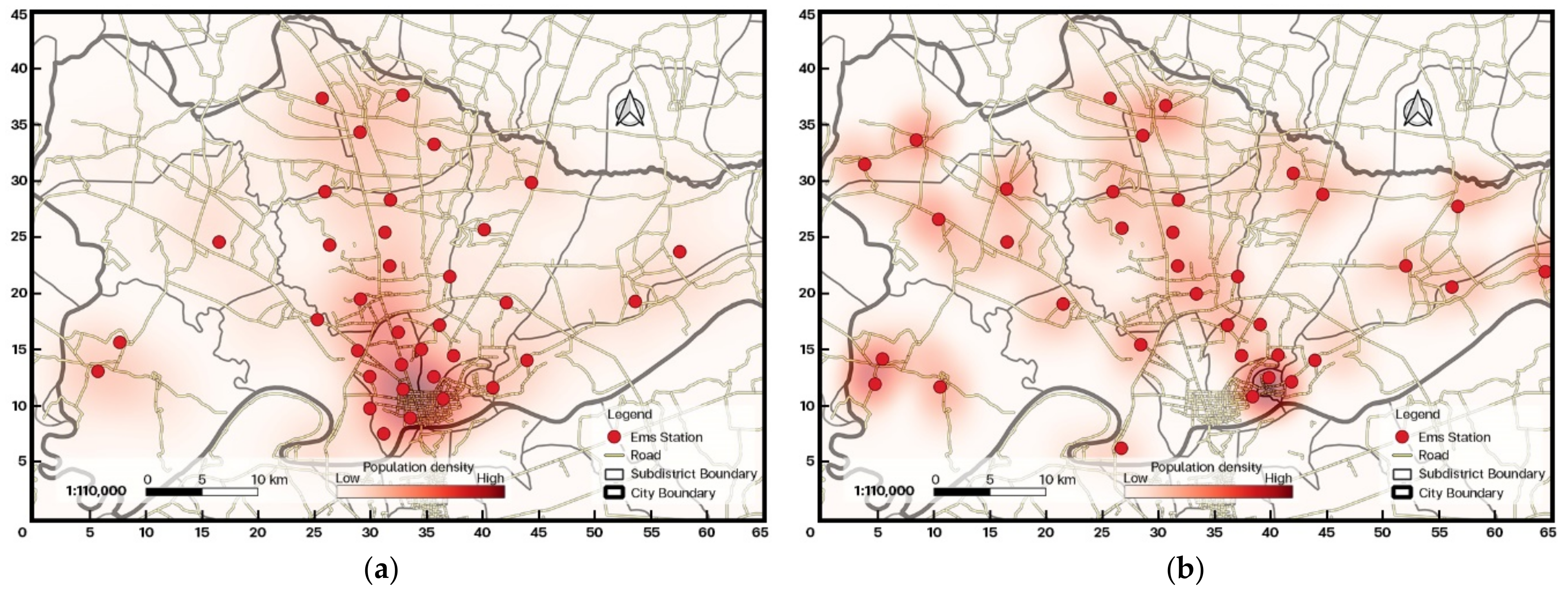
From the computational results, we can see that using the proposed method generated a 40.52% faster arrival time at the patients, which can increase the chances of patient survival. The maximum arrival time decreased from 31.72 min to 16.95 min, or 46.56%, while the minimum arrival time at the patients decreased from 8.10 to 5.04 min, or 37.77%. Finally, the total cost and total distance traveled were reduced by 32.06% and 29.97%, respectively. Comparing the GA and M-VaNSAS, M-VaNSAS generated a 13.43% lower cost than that of the GA and recorded 16.76% less total distance than that of the GA. An example of the locations of the EMSs during the day (a) and at night (b) is shown in Figure 10.

5. Conclusions and Future Outlook

We proposed a methodology to dynamically and optimally locate EMSs in order to reach the patients on time. An IOT was installed to calculate the current traveling time from point to point and connect this information with the designed EMS relocation algorithm. Trained volunteers were assigned to the used EMSs in order to obtain the lowest assignment cost of the whole system while maintaining the service level. The M-VaNSAS was proposed to solve the problem, and the effectiveness was compared with the well-known genetic algorithm (GA).
Four black boxes were used to improve the initially constructed methods. These black boxes were random-transit (RT), best-transit (BT), inter-transit (IT), and scaling factor (SF). The new black box selection formula was modified to obtain a better solution. The link between Pareto analysis and the VaNSAS was first discussed in this paper to achieve combinatorial optimization. The computational result showed that the M-VaNSAS improved the solution quality of the GA by up to 19.69%. The case study results showed that M-VaNSAS obtained 28.56% and 15.03% lower cost than that of the current procedure and GA, respectively.
The proposed methods outperformed the current practice and the genetic algorithm for the following reasons.
(1)
The service time (average time to reach the patients) was reduced because of the application and IOT system designed and used in this study. Real-time traffic reporting to the central computer was used to reroute the ambulance; therefore, the EMS could reach patients more quickly.
(2)
The total cost and distance to service the patients were reduced due to the effectiveness of the designed algorithm (M-VaNSAS).
(3)
The service level of the patients was increased, as the number of people covered within seven minutes increased with M-VaNSAS; this could reduce the number of severe cases.
For future work, we know that patient demand for EMS is not always predictable, and it occurs stochastically in the real word. Therefore, stochastic demand management will be a focus in future research. Moreover, the integration of the EMS dispatching strategy should also be present in order to obtain a good plan for the EMS location and dispatching strategy.

Author Contributions

Conceptualization, R.P. and P.S.; methodology, C.K.; software, P.S.; validation, K.P., S.K. (Sasitorn Kaewman) and T.S.; formal analysis, S.K. (Surajet Khonjun); investigation, K.S.; resources, P.S.; data curation, C.K.; writing—original draft preparation, N.N.; writing—review and editing, P.S.; visualization, C.K.; supervision, N.N.; project administration, K.S.; funding acquisition, T.S. All authors have read and agreed to the published version of the manuscript.

Funding

National Science, Research and Innovation Fund (Grant No. 2450857).

Institutional Review Board Statement

Not applicable.

Informed Consent Statement

Not applicable.

Acknowledgments

The authors are grateful for the support from (1) the Research Unit on System Modelling for Industry (Grant No. SMI.KKU 64/06), Faculty of Engineering, Khon Kaen University, Thailand, (2) the Artificial Intelligence Optimization SMART Laboratory, Faculty of Engineering, Ubon Ratchathani University, (3) the Faculty of Computer Science, Ubon Ratchathani Rajabhat University, and (4) the Fundamental Fund 65 support from the Thai Government.

Conflicts of Interest

The authors declare no conflict of interest.

References

  1. Trujillo, L.; Álvarez-Hernández, G.; Maldonado, Y.; Vera, C. Comparative Analysis of Relocation Strategies for Ambulances in the City of Tijuana, Mexico. Comput. Biol. Med. 2020, 116, 103567. [Google Scholar] [CrossRef] [PubMed]
  2. Bélanger, E.; Ahmed, T.; Vafaei, A.; Curcio, C.L.; Phillips, S.P.; Zunzunegui, M.V. Sources of Social Support Associated with Health and Quality of Life: A Cross-Sectional Study among Canadian and Latin American Older Adults. BMJ Open 2016, 6, e011503. [Google Scholar] [CrossRef] [PubMed] [Green Version]
  3. Nair, R.; Miller-Hooks, E. Evaluation of Relocation Strategies for Emergency Medical Service Vehicles. Transp. Res. Rec. 2009, 2137, 63–73. [Google Scholar] [CrossRef]
  4. Gendreau, M.; Laporte, G.; Semet, F. A Dynamic Model and Parallel Tabu Search Heuristic for Real-Time Ambulance Relocation. Parallel Comput. 2001, 27, 1641–1653. [Google Scholar] [CrossRef] [Green Version]
  5. Zidi, I.; Al-Omani, M.; Aldhafeeri, K. A New Approach Based on the Hybridization of Simulated Annealing Algorithm and Tabu Search to Solve the Static Ambulance Routing Problem. Procedia Comput. Sci. 2019, 159, 1216–1228. [Google Scholar] [CrossRef]
  6. Bélanger, V.; Lanzarone, E.; Nicoletta, V.; Ruiz, A.; Soriano, P. A Recursive Simulation-Optimization Framework for the Ambulance Location and Dispatching Problem. Eur. J. Oper. Res. 2020, 286, 713–725. [Google Scholar] [CrossRef]
  7. Mouhcine, E.; Karouani, Y.; Mansouri, K.; Mohamed, Y. Toward a Distributed Strategy for Emergency Ambulance Routing Problem. In Proceedings of the 2018 4th International Conference on Optimization and Applications (ICOA), Mohammedia, Morocco, 26–27 April 2018; pp. 1–4. [Google Scholar] [CrossRef]
  8. Schmid, V.; Doerner, K.F. Ambulance Location and Relocation Problems with Time-Dependent Travel Times. Eur. J. Oper. Res. 2010, 207, 1293–1303. [Google Scholar] [CrossRef] [Green Version]
  9. Rajagopalan, H.K.; Saydam, C.; Xiao, J. A Multiperiod Set Covering Location Model for Dynamic Redeployment of Ambulances. Comput. Oper. Res. 2008, 35, 814–826. [Google Scholar] [CrossRef]
  10. Chumachenko, D.; Meniailov, I.; Bazilevych, K.; Chumachenko, T.; Yakovlev, S. Investigation of Statistical Machine Learning Models for COVID-19 Epidemic Process Simulation: Random Forest, K-Nearest Neighbors, Gradient Boosting. Computation 2022, 10, 86. [Google Scholar] [CrossRef]
  11. Ma, X.; Zhao, X.; Guo, P. Cope with the COVID-19 Pandemic: Dynamic Bed Allocation and Patient Subsidization in a Public Healthcare System. Int. J. Prod. Econ. 2022, 243, 108320. [Google Scholar] [CrossRef]
  12. Yuk-Chiu Yip, J. Healthcare Resource Allocation in the COVID-19 Pandemic: Ethical Considerations from the Perspective of Distributive Justice within Public Health. Public Heal. Pract. 2021, 2, 100111. [Google Scholar] [CrossRef]
  13. Biswas, R.; Arya, S.; Arya, K. A Quantifiable Framework for ‘COVID-19 Exposure’ to Support the Vaccine Prioritization and Resource Allocation for Resource-Constraint Societies. Urban Gov. 2021, 1, 23–29. [Google Scholar] [CrossRef]
  14. Kim, D.; Pekgün, P.; Yildirim, İ.; Keskinocak, P. Resource Allocation for Different Types of Vaccines against COVID-19: Tradeoffs and Synergies between Efficacy and Reach. Vaccine 2021, 39, 6876–6882. [Google Scholar] [CrossRef]
  15. Chen, P.S.; Lin, Y.J.; Peng, N.C. A Two-Stage Method to Determine the Allocation and Scheduling of Medical Staff in Uncertain Environments. Comput. Ind. Eng. 2016, 99, 174–188. [Google Scholar] [CrossRef]
  16. Vieira, B.; Demirtas, D.; van de Kamer, J.B.; Hans, E.W.; van Harten, W. A Mathematical Programming Model for Optimizing the Staff Allocation in Radiotherapy under Uncertain Demand. Eur. J. Oper. Res. 2018, 270, 709–722. [Google Scholar] [CrossRef] [Green Version]
  17. Evoy, K.E.; Raber, H.P.; Battjes, E.N.; Sheridan, E.P. Volunteering as Medical Staff at a Diabetes Summer Camp as a Component of a Pharmacy Residency Program. Curr. Pharm. Teach. Learn. 2016, 8, 437–441. [Google Scholar] [CrossRef]
  18. Wise, D.; Bruun, T.; Swee, J.; Caceres, W.; Singh, B.; Ahmed, A. Sa1516 Linkage-to-Care for Patients with Viral Hepatitis Provided by the Free Community-Based Hepatology Clinic Organized by Medical Students and Staffed by Volunteer Hepatologists. Gastroenterology 2020, 158, S-1318. [Google Scholar] [CrossRef]
  19. Chow, C.; Goh, S.K.; Tan, C.S.G.; Wu, H.K.; Shahdadpuri, R. Enhancing Frontline Workforce Volunteerism through Exploration of Motivations and Impact during the COVID-19 Pandemic. Int. J. Disaster Risk Reduct. 2021, 66, 102605. [Google Scholar] [CrossRef]
  20. Caunhye, A.M.; Zhang, Y.; Li, M.; Nie, X. A Location-Routing Model for Prepositioning and Distributing Emergency Supplies. Transp. Res. Part E Logist. Transp. Rev. 2016, 90, 161–176. [Google Scholar] [CrossRef]
  21. Oran, A.; Tan, K.C.; Ooi, B.H.; Sim, M.; Jaillet, P. Location and Routing Models for Emergency Response Plans with Priorities. Commun. Comput. Inf. Sci. 2012, 318, 129–140. [Google Scholar] [CrossRef] [Green Version]
  22. Daskin, M.S. Maximum Expected Covering Location Model: Formulation, Properties and Heuristic Solution. Transp. Sci. 1983, 17, 48–70. [Google Scholar] [CrossRef] [Green Version]
  23. Khamsing, N.; Chindaprasert, K.; Pitakaso, R.; Sirirak, W.; Theeraviriya, C. Modified ALNS Algorithm for a Processing Application of Family Tourist Route Planning: A Case Study of Buriram in Thailand. Computation 2021, 9, 23. [Google Scholar] [CrossRef]
  24. Repede, J.F.; Bernardo, J.J. Developing and Validating a Decision Support System for Locating Emergency Medical Vehicles in Louisville, Kentucky. Eur. J. Oper. Res. 1994, 75, 567–581. [Google Scholar] [CrossRef]
  25. Gendreau, M.; Laporte, G.; Semet, F. The Maximal Expected Coverage Relocation Problem for Emergency Vehicles. J. Oper. Res. Soc. 2006, 57, 22–28. [Google Scholar] [CrossRef]
  26. Tlili, T.; Harzi, M.; Krichen, S. Swarm-Based Approach for Solving the Ambulance Routing Problem. Procedia Comput. Sci. 2017, 112, 350–357. [Google Scholar] [CrossRef]
  27. Kazakovtsev, L.; Rozhnov, I.; Popov, A.; Tovbis, E. Self-Adjusting Variable Neighborhood Search Algorithm for Near-Optimal k-Means Clustering. Computation 2020, 8, 90. [Google Scholar] [CrossRef]
  28. Guillot, J.; Restrepo-Leal, D.; Robles-Algarín, C.; Oliveros, I. Search for Global Maxima in Multimodal Functions by Applying Numerical Optimization Algorithms: A Comparison between Golden Section and Simulated Annealing. Computation 2019, 7, 43. [Google Scholar] [CrossRef] [Green Version]
  29. Gómez-Montoya, R.A.; Cano, J.A.; Cortés, P.; Salazar, F. A Discrete Particle Swarm Optimization to Solve the Put-Away Routing Problem in Distribution Centres. Computation 2020, 8, 99. [Google Scholar] [CrossRef]
  30. Pitakaso, R.; Sethanan, K.; Theeraviriya, C. Variable Neighborhood Strategy Adaptive Search for Solving Green 2-Echelon Location Routing Problem. Comput. Electron. Agric. 2020, 173, 105406. [Google Scholar] [CrossRef]
  31. Jirasirilerd, G.; Pitakaso, R.; Sethanan, K.; Kaewman, S.; Sirirak, W.; Kosacka-Olejnik, M. Simple Assembly Line Balancing Problem Type 2 by Variable Neighborhood Strategy Adaptive Search: A Case Study Garment Industry. J. Open Innov. Technol. Mark. Complex. 2020, 6, 21. [Google Scholar] [CrossRef] [Green Version]
  32. Worasan, K.; Sethanan, K.; Pitakaso, R.; Moonsri, K.; Nitisiri, K. Hybrid Particle Swarm Optimization and Neighborhood Strategy Search for Scheduling Machines and Equipment and Routing of Tractors in Sugarcane Field Preparation. Comput. Electron. Agric. 2020, 178, 105733. [Google Scholar] [CrossRef]
  33. Hwang, C.-L.; Yoon, K. Methods for Multiple Attribute Decision Making. In Multiple Attribute Decision Making; Springer: Berlin/Heidelberg, Germany, 1981; pp. 58–191. [Google Scholar] [CrossRef]
  34. Mitchell, R.J.; Chambers, B.; Anderson, A.P. Array Pattern Synthesis in the Complex Plane Optimised by a Genetic Algorithm. Electron. Lett. 1996, 32, 1843–1845. [Google Scholar] [CrossRef]
  35. Schorcht, G. Heltec WiFi LoRa 32 V2 Boards. Available online: https://doc.riot-os.org/group__boards__esp32__heltec-lora32-v2.html#esp32_heltec_lora32_v2_overview (accessed on 1 May 2022).
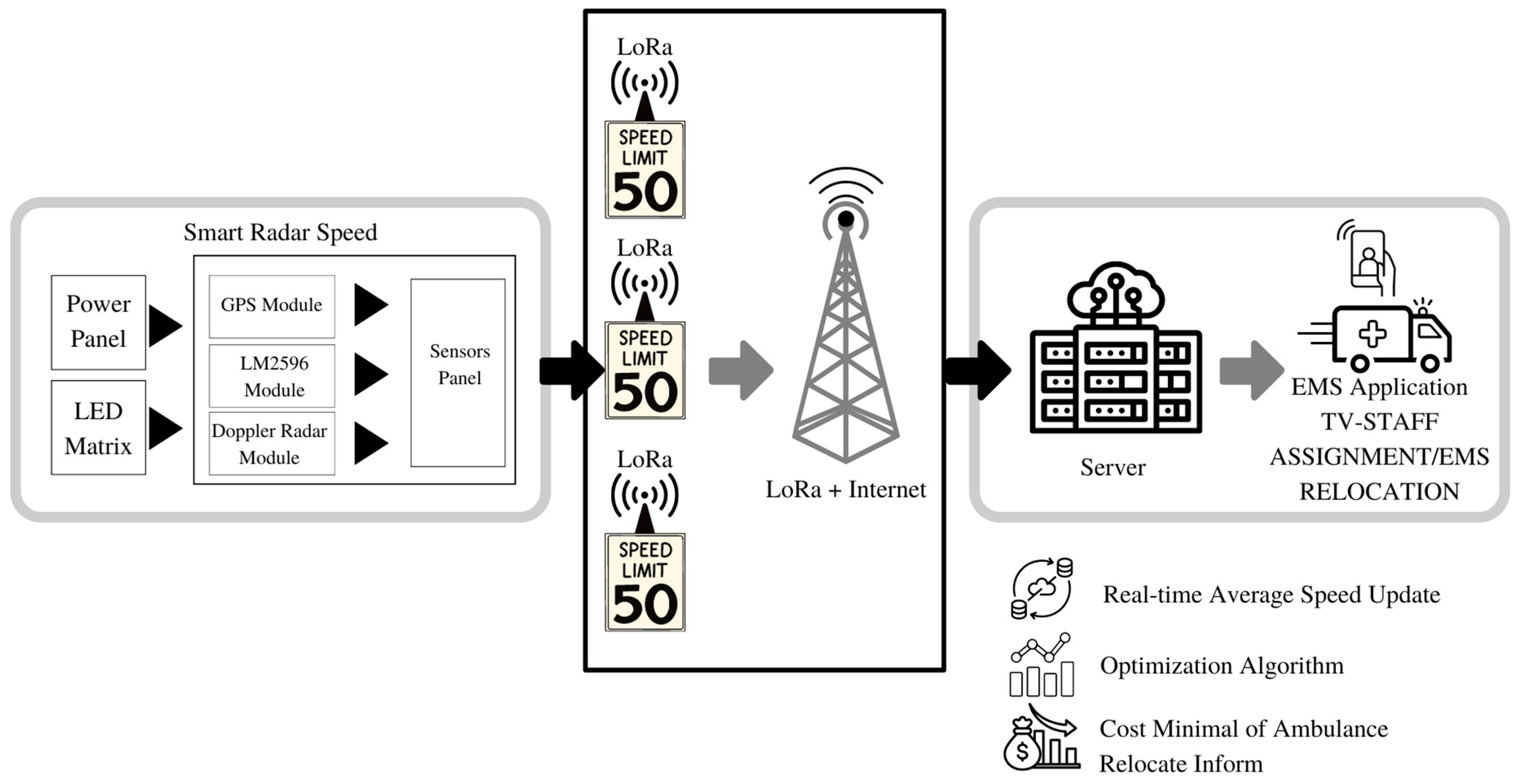
Figure 1. Framework of the proposed problem.
Computation 10 00103 g001
Figure 2. The proposed architecture design.
Computation 10 00103 g002
Figure 3. User interface EMS application design.
Computation 10 00103 g003
Figure 4. Effect of weight w1 on the total cost given by different solution approaches.
Computation 10 00103 g004
Figure 5. Effect of weight w1 on the number of populations covered by the ambulances within R1 traveling time (Cov-R1) given by different solution approaches.
Computation 10 00103 g005
Figure 6. Pareto front of GA.
Computation 10 00103 g006
Figure 7. Pareto front of M-VaNSAS.
Computation 10 00103 g007
Figure 8. Progressive plot of the development of the best average cost per person found during the search with the proposed methods.
Computation 10 00103 g008
Figure 9. Average cost per population (baht/person).
Computation 10 00103 g009
Figure 10. Day and night EMS location.
Computation 10 00103 g010
Table 1. NP of initial tracks.
Elements12345
Track No
10.770.070.820.140.44
20.280.760.550.960.52
30.830.600.430.770.63
40.120.910.580.410.98
Table 2. Traveling time of time t of the location i to locate the EMS j.
Community123456789
Location
142078186171624
211172121231261320
37101518191512244
419175222116131716
5891065166239
Table 3. Community assignment results.
Community123456789#Patients#Community
EMS
11 1 1 1 6104
2 11 13993
3 111 1 6004
41 1 113894
5 1 11 4003
Table 4. Sorting results of the value of elements of track 1.
Before sortElements12345
Value0.770.070.820.140.77
After sortElement24513
Value0.070.140.770.770.82
Table 5. Results of the decoding method.
Community123456789#Patients#Community
EMS
11 1 1111 8406
2 00
3 111 1 118596
4 00
511 11 1 17996
Table 6. TV assignment results.
Community123456789Exp.TVInExp.TVTotal Exp.
EMS
11 1 1111 3 (1.3)1 (0.8)2.1
3 111 1 116 (1.4)4 (0.7)2.1
511 11 1 12(1.3)5 (0.9)2.2
Table 7. List of variables that need to be iteratively updated.
VariablesUpdate Procedure
N b t Total number of tracks that select black box b from iteration 1 to iteration t
A b t A b t = N b t T b t .
when T b t is total cost generated from all tracks that select black box b (iteration 1 to iteration t)
I b t I b t = I b t 1 + G
when G = 1     i f   b l a c k   b o x   b   c o n t a i n   g l o b a l   b e s t   s o l u t i o n   i n   i t e r a t i o n   t   0
B j g b e s t Update global best track
R i j q     Randomly select the value in position of all track, all position
Table 8. Details of 14 randomly generated test instances.
#Instance#Community#Inhabitant#EMS#Instance#Community#Inhabitant#EMS
A-145356114A-810016,36125
A-250377314A-910017,05825
A-37510,58120A-1010017,98125
A-47511,24620A-1110018,37527
A-58012,49820A-1212018,89127
A-68014,35623A-1312021,23927
A-78015,02923A-1414828,49132
Remark: # means number of.
Table 9. Random parameter settings.
ParametersDefined ValueParametersDefined Value
IU [8, 48]R2: PST15 min,
JU [20, 153]LU [50, 120]
H28 minT24 h
R17 minO5 communities
PjtU [50, 450]M2.5
ElU [0.8, 1.2]D3 persons
Tijt:1 km/minClU [350, 550]
B:8 Baht/minAiU [500, 1500]
Table 10. Computational results of all 14 test instances when varying w1 and w2.
#instanceGAM-VaNSAS
w1 = 0.3; w2 = 0.7w1 = 0.5; w2 = 0.5w1 = 0.7; w2 = 0.3w1 = 0.3; w2 = 0.7w1 = 0.5; w2 = 0.5w1 = 0.7; w2 = 0.3
f i q 1 f i q 2 f i q 1 f i q 2 f i q 1 f i q 2 f i q 1 f i q 2 f i q 1 f i q 2 f i q 1 f i q 2
A-114,781281712,422261912,006259113,783324812,297305312,0182998
A-215,915312914,196300413,827283314,481344113,491321913,1203105
A-320,177738119,894678118,759659318,718917217,809872816,9158201
A-423,481819822,372771221,981734619,96410,27619,182987118,7829134
A-524,147927423,394906322,855853922,12011,92421,85311,03621,10510,863
A-625,60111,09224,71210,75324,016998223,31813,29122,37512,85721,98212,019
A-726,01812,84125,98411,28425,09110,98224,72314,87423,81213,46422,98113,006
A-828,84313,91827,81913,05427,04712,45726,91815,98226,11814,82425,33614,048
A-930,02714,77129,87114,04829,28413,87128,86416,49927,08516,01026,84915,812
A-1031,23815,05230,84514,28130,01814,02829,01616,82128,34716,12427,81716,036
A-1134,91916,98934,07416,04233,85315,78131,18317,29531,02817,03830,07516,982
A-1235,62017,00134,59116,89134,43716,05732,01917,83732,11317,24931,09717,028
A-1337,87118,96436,72618,05836,11217,98234,90120,19333,78219,51733,04419,040
A-1450,92824,21948,78623,12446,79023,00643,92827,98142,01826,75741,28225,593
average28,540.4312,546.1427,549.0011,908.1426,862.5711,574.8625,995.4314,202.4325,093.5713,553.3624,457.3613,133.21
%diff16.6911.6612.6416.159.8318.506.290.002.604.570.007.53
Table 11. Comparison of Pareto ratio of GA and M-VaNSAS.
IterationGA M-VaNSAS
Number of Pareto PointsARPNumber of Pareto PointsARP
2002801.43401.7
5006011.208911.78
8009331.1710231.28
100012841.2815061.51
120014901.2417011.41
150016801.1220141.34
Average12031.2813621.46
Table 12. Average cost per person of the population in the communities.
Best Result from Lingo v.16GAM-VaNSAS
A-15.284.744.03
A-25.014.734.19
A-33.452.932.04
A-43.522.901.94
A-53.742.581.98
A-63.022.301.74
A-73.182.301.77
A-83.422.131.76
A-93.452.131.69
A-103.122.161.76
A-114.042.121.82
A-123.562.051.86
A-134.212.031.73
A-144.512.111.57
average3.822.662.13
Table 13. p-value of the statistical test using Wilcoxon signed-rank test of data given in Table 11.
GAM-VaNSAS
Lingo v.160.000960.00096
GA 0.00096
Table 14. Details of the subalgorithm of M-VaNSAS.
IB TypesRandom-Transit (RT)Best-Transit (BT)Inter-Transit (IT)Scaling Factor (SF)
M-VaNSAS-1
M-VaNSAS-2
M-VaNSAS-3
M-VaNSAS-4
M-VaNSAS-5
M-VaNSAS-6
M-VaNSAS-7
M-VaNSAS-8
M-VaNSAS-9
M-VaNSAS-10
M-VaNSAS-11
M-VaNSAS-12
Table 15. Average cost per population (baht/person) of using the different proposed methods.
M-VaNSAS Subalgorithm
Use 1 IBUse 2 IBUse 3 IBUse 4 IB
12345678910111213
A-15.195.235.215.194.874.764.974.754.414.364.444.564.03
A-25.045.115.075.324.984.834.784.694.344.284.384.324.19
A-34.454.584.624.374.133.893.843.893.523.143.262.872.04
A-43.513.273.243.182.892.542.492.42.222.182.262.291.94
A-53.253.173.213.182.942.852.582.472.181.992.242.451.98
A-62.782.922.652.592.432.572.492.282.112.082.422.311.74
A-72.692.542.852.732.462.312.512.262.031.932.252.181.77
A-82.712.882.962.232.522.472.282.542.152.322.082.021.76
A-92.652.712.592.642.282.322.392.312.182.262.292.181.69
A-102.512.672.622.52.422.382.542.442.062.182.252.081.76
A-112.642.692.582.662.572.42.592.382.192.282.042.431.82
A-122.782.52.632.732.642.662.712.732.262.312.182.371.86
A-132.592.642.782.562.552.482.732.512.32.372.162.081.73
A-142.382.352.472.292.432.152.272.321.921.852.11.891.57
Ave.3.233.233.253.163.012.902.942.862.562.542.602.572.13
% dif51.6451.6452.5848.3641.3136.1538.0334.2720.1919.2522.0720.660.00
Note: the %dif is the relatively different result of the subalgorithm with the best solution.
Table 16. Comparative results of the current situation and the proposed method.
Average Arrival Time to Patients (min)Maximum Arrival Time to Patients (min)Minimum Arrival Time to Patients (min)Total Cost Incurred (baht)Total Distance (km)
Current situation22.4831.728.101,718,3868298
GA18.6025.017.051,348,7276981
M-VaNSAS13.3716.955.041,167,4795811
Publisher’s Note: MDPI stays neutral with regard to jurisdictional claims in published maps and institutional affiliations.