Optimizing DSO Requests Management Flexibility for Home Appliances Using CBCC-RDG3

Abstract

This article covers a case study with homes equipped with multiple appliances for energy consumption. The central goal is to provide for aggregators’ flexibility in distribution networks by building an optimal schedule that takes advantage of load flexibility resources. This, in turn, allows for the re-scheduling of shifting/real-time home appliances to provision a request from a distribution system operator (DSO). The paper concludes with the consideration of the CBCC-RDG3, HyDE-DF, and genetic algorithms, which were used to find the best schedule that would be highly efficient and meet all the constraints associated with the problem that successfully demonstrate the effectiveness of this particular approach.

1. Introduction

The dawn of Smart Grids (SG) together with the high penetration of Distributed Generation (DG) poses a new level of complexity in power system operation planning [1]. Broadly speaking, the complexity resides in the consideration of stochastic variables in the mathematical formulation of optimization problems (associated with the increasing penetration of renewables) [2]. Paper [3] introduces two testbeds, which constitute a valuable reference for testing and comparing heuristic optimization algorithms.

There are several methods of demand management and algorithms used in the literature [4,5,6,7,8,9,10,11]. Most of them are system-specific [4,5,6,8,11] strategies, and some of them do not apply to practical systems with a large number of independent devices. Most of the methods have been developed using dynamic programming [11] and linear programming [5,8]. These programming methods cannot handle a large number of managed devices from multiple device types that have multiple calculation patterns and heuristics. The primary goal of demand management techniques presented in the literature is to reduce system peak demand and operating costs. While utilities may offer various incentives to relevant customers to directly control [5,10,11,12] selected loads by grouping customer loads, most methodologies used in the literature do not consider criteria and targets independently. Thus, it is difficult to use these methods for demand management in future smart grids, which aim to give consumers more control over their energy consumption. In a smart grid, demand management strategies must handle a large number of controlled loads of several types. In addition, loads may have characteristics extending over several hours. Therefore, the strategies must be able to deal with all possible durations of managing the various controlled loads.

The artificial neural network (ANN) optimization method and NSGA II heuristic planning are used for load prediction [13]. Heuristic strategies used for optimal energy planning for each building in a neighborhood [14]. A load switching method is used for Demand Side Management (DSM) [15]. The day-ahead load-shifting techniques were mathematically formulated as a minimization problem. A heuristic-based Evolutionary Algorithm (EA) that easily adapts heuristics in the problem is developed for solving this minimization problem, and simulations are carried out. The algorithm can handle a large number of controllable devices of several types and achieves substantial savings while reducing the peak load demand.

The Genetic and Evolutionary Computation Conference 2021 [16] organized a challenge dedicated to the flexibility management of home appliances to support DSO requests [17]. The main goal of this competition is to provide models for an aggregator’s flexibility provision in distribution networks that take advantage of load flexibility resources, allowing the re-schedule of shifting/real-time home-appliances to provision a request from a distribution system operator (DSO).

Among stochastic optimization methods, methods that use laws and principles borrowed from nature itself, such as evolutionary optimization methods, swarm intelligence methods [18,19], particle swarm intelligence [20,21], annealing simulation algorithms, and genetic algorithms [22] have proven themselves especially useful in practice. The first two groups belong to the so-called population methods since they use systems consisting of agents (populations of agents). As a rule, an agent is understood as a certain point in the search space for solutions to the problem, and the optimization process consists of moving agents in this space.

The methods were chosen as follows: we first undertook a review of the literature as well as other recent comparable competitions. The Large-Scale Global Optimization competition was found [23], according to the results of which the CBCC-RDG3 algorithm was selected as a potentially good method for stating our problem.

The novelty of our research work is related to the application of the generally new and efficient global optimization algorithms to the applied industry-related research problem. We made an extensive comparison of the existing heuristic algorithms and drew the conclusion that the HyDE-DF algorithm has a better performance.

2. Competition

The owner of the challenge problem is the Genetic and Evolutionary Computation Conference (GECCO). GECCO has presented the latest high-quality results in genetic and evolutionary computation since 1999 [16]. The GECCO 2021 competition proposed a track in the energy domain: flexible control of home appliances to support DSO requests.

The issue concerns the aggregator that controls device management with demand response (DR) capabilities [24]. Users voluntarily enroll in Flexibility by receiving monetary compensation if their base profile changes.

The features and assumptions of the optimization model in a competitive environment follow:

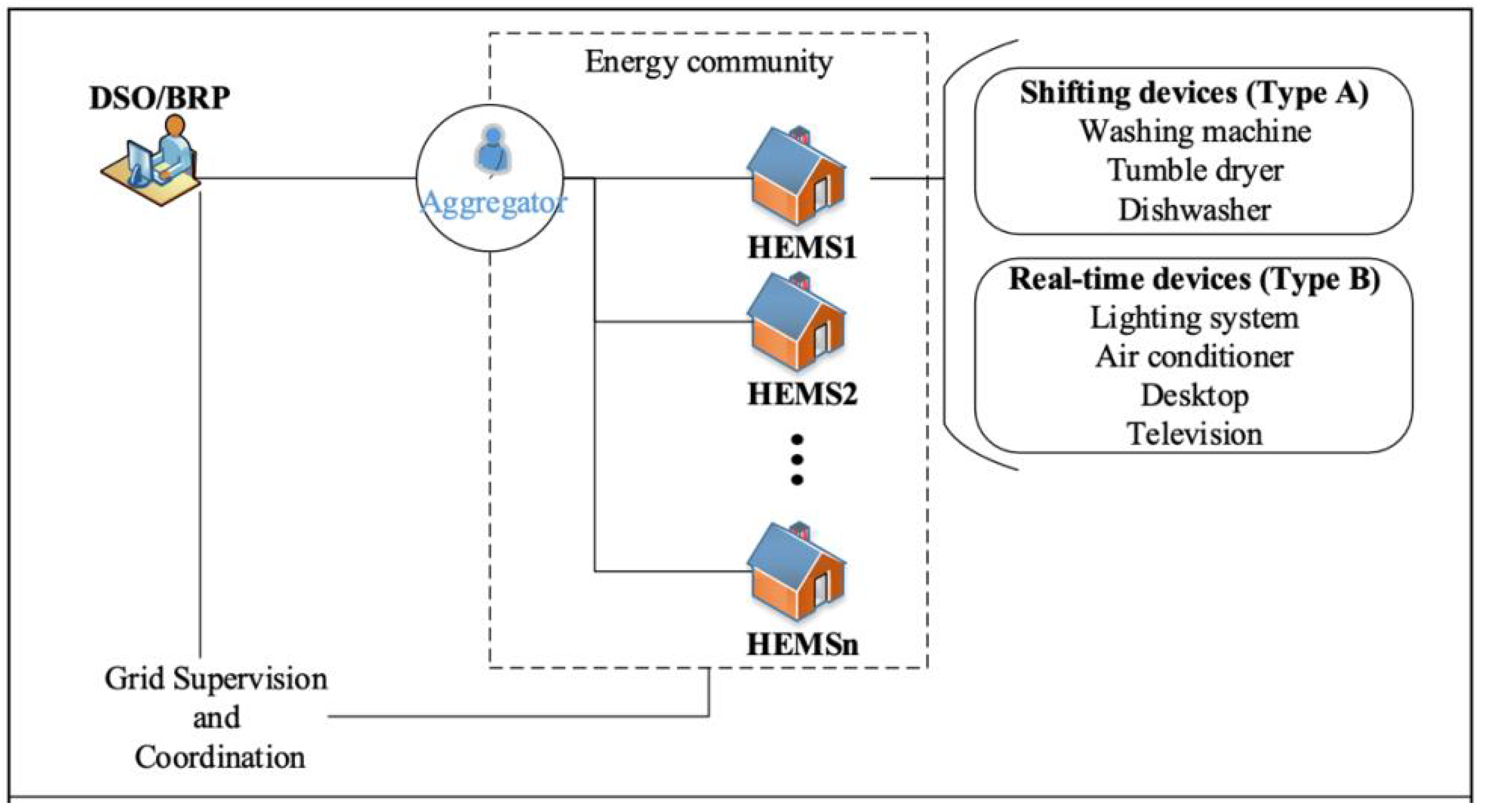
• Perspective of an aggregator in charge of HEMS with various devices with disaster recovery capabilities.
• Two types of devices are considered for disaster recovery: devices whose consumption can be rolled over to another period, and devices with the ability to manage in real time.
• The aggregator responds to a flexibility request from the DSO or BRP, which pays monetary compensation for each unit of capacity (PU) of flexibility provided.
• The aggregator uses a flex management system to reschedule some devices and approximate the flex curve provided by the DSO as closely as possible.
• Users can register their devices for flexibility and set preferences for the allowed shift times, expected rewards for flex activation, and the prioritization of available devices for activation, among other things.
• Assuming that the necessary infrastructure to achieve such command and control (e.g., smart metering systems, communication lines, HEMS) is in place.
• Both the DSO/BPR and the aggregator have access to the predicted baseline power consumption provided by a third party.

The case study looks at homes equipped with household appliances in one of the categories mentioned above. In particular, we assume houses with the following main equipment for energy consumption (Figure 1):

(A) Mobile devices: dishwashers, washing machines, and dryers;

(B) Real-time devices: lighting devices, televisions, and computers.

2.1. Description of Parameters

For a specific task, this solution should contain all new launch periods for type A devices: with shifting capabilities and type B: with the new intensities of real-time appliances.

2.1.1. Type A Appliances

The information related to appliances type A can be encoded in a vector that indicates the new starting times of each device:

$$x_{shift}=\left[T_{new\left(1\right)},T_{new\left(2\right)},\dots ,T_{new\left(i\right)}\right]$$

$x_{shift}$ contains the decision variables corresponding to the new starting period of appliance $i\in A$ (Type A).

2.1.2. Type B Appliances

New intensities for appliances type B should be defined for all of their operation periods and are encoded as:

$$\begin{array}{c}{x}_{int}=[In{t}_{new(1,1)},\dots ,In{t}_{new(1,N_T)},In{t}_{new(2,1)},\dots ,\hfill \\ \hfill In{t}_{new(2,N_T)},\dots ,In{t}_{new(N_j,1)},\dots ,In{t}_{new(N_j,N_T)}]\end{array}$$

where $x_{int}$ contains the decision variable $In{t}_{new(j,t)}$ that represents the new intensity of the jth appliance in the operation period t.

2.2. Solution Representation

The vectors $x_{shift}$ and $x_{int}$ are concatenated to form a new vector that represents a solution (Figure 2).

$$X=[x_{shift},x_{int}]$$

2.3. Objective Function

We evaluate solutions with fitness function $f\left(x\right)$ that acts like a black box, as shown in Figure 3.

3. Mathematical Optimization Problem

The following mathematical optimization problem was proposed in the research paper [24] and by the competition organizers [17].

$$\begin{array}{c}\mathit{Minimize}f=\left(\sum _{i=1}^{N_1}{Re{m}_A}_{\left(i\right)}+\sum _{i=1}^{N_1}{Re{m}_B}_{\left(i\right)}\right)+C_{DSO}·F_{match};\end{array}$$

(1)

$$\begin{array}{c}{Re{m}_A}_{\left(i\right)}=\left\{\begin{array}{cc}{C_A}_{\left(i\right)},\hfill & if{t}_{start\left(i\right)}\ne t_{new\left(i\right)}\hfill \\ 0,\hfill & \mathrm{otherwise}\hfill \end{array}\right.;\end{array}$$

(2)

$$\begin{array}{c}Re{m}_{B_{\left(i\right)}}=C_{B\left(i\right)}·\sum _{i=1}^{N_T}\mid B_{base(j,t)}-B_{flex(j,t)}\mid ;\end{array}$$

(3)

$$\begin{array}{c}{F}_{match}=\sum _{i=1}^{N_T}\mid F_{agg\left(t\right)}-F_{DSO\left(t\right)}\mid ;\end{array}$$

(4)

$$\begin{array}{c}l{b}_i\le X_i\le u{b}_i,i=\overline{1,940}.\end{array}$$

(5)

The solution is evaluated using the fitness function (Equation (1)). In order to maximize the aggregator profits, the fitness function is modeled as the minimization of the remuneration to be paid to the households plus a penalty for the mismatch of flexibility procured by the DSO/BRP ($F_{match}$). Here, Equation (2) corresponds to the monetary compensation paid for shifting device i (a flat payment $C_{A\left(i\right)}$ in EUR is considered despite how many periods the device is shifted); Equation (3) corresponds to the remuneration given for the modification of the baseline profile of devices type B (where $C_{B\left(j\right)}$ is a compensation paid in EUR/kWh modification); and Equation (4) corresponds to a penalty, $C_{DSO}$ in EUR/kWh, paid for the mismatch between the flexibility procured by the $DSO$ ($F_{DSO\left(t\right)}$) and the flexibility provided by the aggregator ($F_{agg\left(t\right)}$) in each period t.

A solution is represented as a vector $X=[x_{shift},x_{int}]$ (Figure 2). For each component of the $x_{shift}$ vector, there are constraints in the form of a lower bound (lb) and an upper bound (ub).

Optimization problem details:

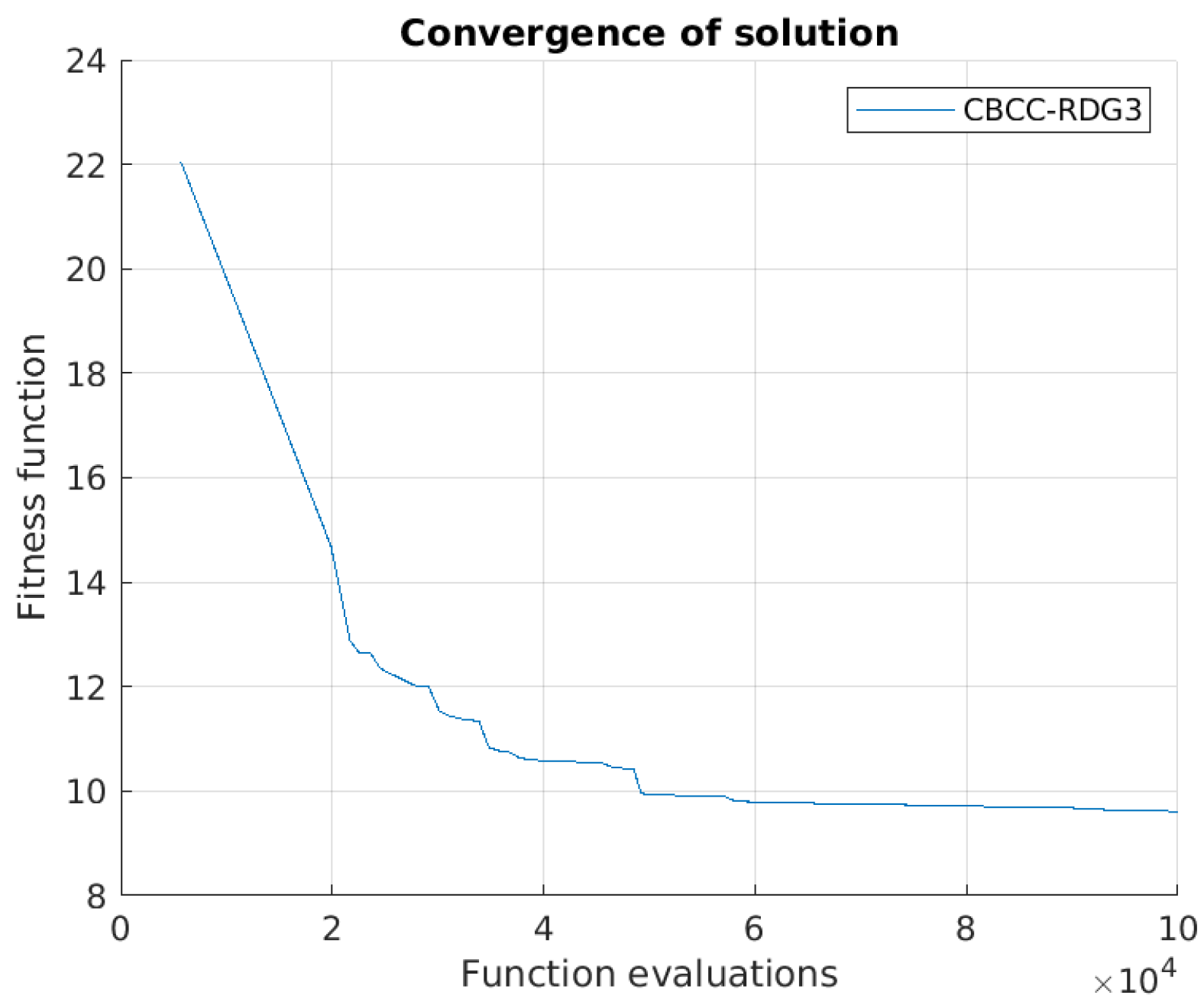
• The competition organizers provided information that a maximum number of 100,000 function evaluations are allowed in the competition.
• The total dimension of the problem is 940.

Finally, we obtain a continuous optimization problem (Equations (1)–(5)). Because of the complexity and types of equations integrated into the objective function, we will examine our problem as a problem of nonlinear continuous optimization. Due to the complexity of the optimization problem, we consider it a black-box optimization problem. Therefore, we will use an evolutionary algorithm as a core optimization method.

4. Solution Approach

4.1. Known Methods

When analyzing competitions in the field of global, combinatorial and black optimization, we have chosen a solution [25] to this problem that is of high quality at the moment. A detailed analysis of cases of the competitive process generates new ideas, which then help to obtain effective solutions. In particular, the IEEE CEC’2019 Special Session and Competition on Large-Scale Global Optimisation were considered, according to the results of which CBCC-RDG3 became the leading algorithm.

We decided to use the winner of the CEC’2019 competition, since the algorithm had shown good results in all considered categories, including the one of our interest. As a result, to solve our problem, we chose the CBCC-RDG3 algorithm, which was the winner of one of the considered problems. Moreover, the GA (a classical solution) and HyDE-DF (a solution, given by the organizers) algorithms were chosen as comparisons. We deliberately did not compare CBCC-RDG3 with other algorithms, but only with HyDE-DF, since [26] has already compared EPSDE [27], MPEDE [28], and CLPSO [29] with HyDE-DF, and it was concluded from the results that HyDE-DF shows better results.

4.2. CBCC-RDG3

The CBCC-RDG3 [30] uses a “divide and conquer” strategy and consists of two stages: decomposition via RDG3 (Modified Recursive Differential Groupping) and optimization, using CMA-ES Algorithm 1:

Algorithm 1 CBCC-RDG3.

1: divide decision parameters X into subsets $X_i$: $1<=i<=m$, using RDG3 2: $x^{*}$—a context vector 3: fori from 1 to $ite{r}_{max}$ do 4:      for i from 1 to m do 5:            Find optimal solution for the sub-component using CMA-ES 6:            Update $x^{*}$ 7:      end for 8: end for 9: return $x*$

Below, you can see the description of algorithm components.

4.2.1. RDG3

Variables are divided into groups based on their interaction with each other. Two variables, $x_i$ and $x_j$, are considered to interact if the fitness change induced by perturbing $x_i$ varies for different values of $x_j$.

At first, we examine $x_1$ to interact with all the other variables. If no interaction is found, then $x_1$ is placed to separable variables S, and we move to the next variable $x_2$. Otherwise, all the rest of the variables are randomly divided into two equal-sized groups, $G_1$ and $G_2$. Then, we search for the interaction between $x_1$ and these two groups. The process is continued recursively until all the variables interacting with $x_1$ are found. They are placed to $X_1$ with $x_1$.

In the next step, if $\mid X_1\mid <{ϵ}_n$, where ${ϵ}_n$ is the threshold for group size, we try to find the interaction between $X_1$ with the remaining variables to discover variables that interact with $x_1$ indirectly. In case such variables are found, we include them in $X_1$. We continue the process until $\mid X_1\mid >={ϵ}_n$ or until we run out of variables.

After that, we repeat the process with the next variable $x_2$ while we do not reach the last one.

4.2.2. CMA-ES

The algorithm works as follows: the parameters of the multivariate normal distribution over search space is generated, and a population of candidate vectors is randomly sampled from the distribution (line 9 of the Pseudocode) [31,32,33,34]. Then, the fitness function is evaluated for each vector from the population in order to update the mean value and covariance matrix of the distribution (line 17). Since CMA-ES belongs to the class of Evolutionary Strategies (ES), the method includes such steps as mutation, recombination, and selection.

CMA-ES is concerned with matching the search to the level lines of the multivariate target function to be minimized Algorithm 2. The geometric meaning of the covariance matrix determines the algorithm, since the matrix describes an ellipsoidal scattering obeying the normal distribution law. So, by each step changing the covariance matrix, we are looking for an ellipsoid that is as similar as possible to the shape of the objective function level. This will make it easier to find an extremum.

Algorithm 2 CMA-ES.

1: Assigning initial parameters: 2: $p_a^{\left(0\right)}=0;p_c^{\left(0\right)}=0$; – Evolutionary paths 3: $C^{\left(0\right)}=I$; – Covariative Matrix 4: ${\sigma }^{\left(0\right)}\in {\mathbb{R}}_{+};m^{\left(0\right)}\in {\mathbb{R}}^n$ – Step size and mean distribution 5: $g=0;$ – generation 6: while$t<t_{max}$do 7:      A new population of the desired values: 8:      $x_k^{(g+1)}\sim m^{\left(g\right)}+{\sigma }^{\left(g\right)}\mathcal{N}\left(0,C^{\left(g\right)}\right)fork=1\dots \lambda$ 9:      After selection and recombination, obtain new mean: 10:      $m^{(g+1)}={\displaystyle \sum _{i=1}^{\mu }}{\omega }_i·x_{i:\lambda }^{(g+1)}$ 11:      The step size ${\sigma }^{(g+1)}$ is recalculated 12:      $p_{\sigma }^{(g+1)}=(1-c_{\sigma })p_{\sigma }^{\left(g\right)}+\sqrt{c_{\sigma }(2-c_{\sigma })\mu }{C}^{{\left(g\right)}^{-\frac{1}{2}}}$ 13:      ${\sigma }^{(g+1)}={\sigma }^{\left(g\right)}exp\left(\frac{c_{\sigma }}{d_{\sigma }}\left(\frac{\parallel p_{\sigma }^{(g+1)}\parallel }{E\parallel \mathcal{N}(0,I)\parallel }-1\right)\right)$ 14:      Recalculation of the covariance matrix: 15:      $p_c^{(g+1)}=(1-c_c)p_c^{\left(g\right)}+\sqrt{c_c(2-c_c)\mu }\frac{m^{(g+1)}-m^{\left(g\right)}}{{\sigma }^{\left(g\right)}}$ 16:      $C^{(g+1)}=(1-c_{cov})C^{\left(g\right)}+c_{cov}{p}_c^{(g+1)}{p}_c^{{(g+1)}^T}$ 17:      $t=time;$ 18: end while

4.3. Genetic Algorithm

Genetic algorithm (GA) [35] is one of the most common methods of optimization. It consists of the following steps:

1.

Initialization

A set of vectors $X_{i,G}=[x_{1,G},x_{2,G},\dots ,x_{NP,G}]$ called population is randomly generated, where G is the number of generations and NP is the size of the population. Then, we calculate the fitness function for every vector from the population.

2.

Selection

In this step, we leave in the next generation either the parent vector or trial vector according to their fitness value.

3.

Recombination

Trial vectors are generated on the basis of our current generation using a recombination operator: the mutation vector is combined with the individual from the population.

4.

Mutation

At every generation for each vector, we generate mutation vectors using a mutation operator.

Steps 2–4 are repeated until we reach the maximum number of iterations or function evaluations.

In our case, to compare the results, we used default methods from the Genetic Algorithm TOOLBOX For MATLAB [36].

1.

Initialization

This is performed by generating a required number of individuals using a random number generator that uniformly distributes numbers in the desired range, in our case $l{b}_i\le x_{i,G}\le u{b}_i$.

2.

Selection

Stochastic Universal Sampling was used. It is a single-phase sampling algorithm with minimum spread and zero bias.

3.

Recombination

The default crossover function ’crossover scattered’ generates a random binary vector and selects the genes where the vector is a 1 from the first parent and the genes where the vector is a 0 from the second parent, further combining the genes to form the child.

4.

Mutation

For that, we used Gaussian mutation. That method adds a random number obtained from a Gaussian distribution with a mean 0 to every part of the parent vector.

4.4. HyDE-DF

Hybrid-Adaptive DE with Decay Function (HyDE-DF) [37] is an advanced HyDE [38] algorithm. Below is the pseudocode of Algorithm 3.

Algorithm 3 HyDE-DF.

1: Set the control parameters $F_i^1,F_i^2,F_i^3,C{r}_i=0.5$ and NP. 2: Generate the initial population Pop. 3: Evaluate fitness of every individual. 4: Save the best fitness individual $x_{best}$ 5: for$G=1:GEN$do 6:      Calculate decay factor ${\delta }_G$ (lineary decreasing factor) 7:      Generate $F_i^1$, $F_i^2$, $F_i^3$ and $C{r}_i$$\forall i\in$ Pop 8:      for $i=1:$ NP do 9:            Select two individuals: $x_{r1,G}\ne x_{r2,G}$. 10:          Apply mutation operator (6). 11:          Apply recombination (same as standard DE). 12:          Verify boundary constraints. 13:          Apply selection operator (same as standard DE) and update Pop. 14:      end for 15:      Update $F_i^1$, $F_i^2$, $F_i^3$ and $C{r}_i$$\forall i\in$ Pop (same as jDE) 16:      Update best individual $x_{best}$ 17:      if $D{F}_t$ iterations passed, ${\delta }_G=1$, o.w., decrease ${\delta }_G\to 0$ 18:      Apply reinitialization of population if in $R_N$ successive iterations there is no objective value improvement. 19: end for

The difference between HyDE-DF and HyDE is in the mutation function; HyDE-DF uses the mutation operator known as “DE/target-to-perturbedbest/1” (similar to HyDE), with a decay coefficient ${\delta }_G$, the function decreases gradually from 1 to 0 in a period of iterations. The operator is as follows:

$$\begin{array}{c}{\overrightarrow{m}}_{i,G}={\overrightarrow{x}}_{i,G}+{\delta }_G·\left[F_i^1(ϵ·{\overrightarrow{x}}_{best}-{\overrightarrow{x}}_{i,G})\right]+F_i^2({\overrightarrow{x}}_{r1,G}-{\overrightarrow{x}}_{r2,G})\end{array}$$

(6)

where $F_i^1$, $F_i^2$, and $F_i^3$ are scale coefficients in the range [0, 1] independent for each individual i and renew every iteration following the self-adaptive parameter mechanism of the jDE [39] algorithm. ${\overrightarrow{x}}_{r1,G}$ and ${\overrightarrow{x}}_{r2,G}$ are two different random individuals from the population and also different from the current target vector $x_{i,G}$. $x_{best}$ and the best found solution. $ϵ=N(F_i^3,1)$ is a random perturbation coefficient obtained from a normal distribution with mean $F_i^3$ and standard deviation 1. The factor ${\delta }_G$ is used to gradually decrease the influence of the term $F_i^1(ϵ·{\overrightarrow{x}}_{best}-{\overrightarrow{x}}_{i,G})$ responsible for the fast convergence toward the best individual in the population. In addition, the HyDE-DF includes a reinitialization mechanism that is activated if some successive iterations show no improvement in the objective function. In this case, the population is replaced by generating new individuals around a given number of the best-found solutions. The new individuals are generated using random numbers that follow a normal distribution with the mean of those best solutions and a standard deviation of $10\times {10}^{-4}$. The best individual in the population after reinitialization is kept to preserve memory.

5. Simulation Results

For calculations, we used a computer with CPU—Intel(R) Xeon(R) Platinum 8259CL CPU @ 2.50 GHz; RAM—128 GB; OS—Ubuntu 16.04. For the implementation of the algorithms, MATLAB R2021a was used.

In the CBCC-RDG3 algorithm, we tuned ${ϵ}_n$ to be the threshold—the maximum set of non-separated variables, also considering the original article [30]. In CMA-ES, we used parameters in accordance with the original paper [40]. In HyDE-DF and GA, the parameters were not tuned.

The graphs below show a comparison of convergence in the solution of a 50,000 function evaluation (Figure 4 and Figure 5) and of a 100,000 function evaluation (Figure 6 and Figure 7). You can notice that in the graphs for CBCC-RDG3, the line starts at about 6000 scores, because we are considering the work of the RDG3 algorithm for grouping variables.

Below are more detailed results of the algorithms.

Table 1. The table of obtained solutions for CBCC-RDG3.

iRuns	Fit	avgConveRate	timeSpent
Run 1	8.86501141	−0.131981	134.466
Run 2	8.08449529	−0.141198	131.738
Run 3	7.0025118	−0.152127	135.624
Run 4	9.1514026	−0.122969	127.689
Run 5	8.0904988	−0.142578	133.0495
Run 6	7.936813	−0.134536	127.6906
Run 7	8.1752147	−0.141713	133.892
Run 8	8.6713717	−0.127540	121.833
Run 9	8.7980497	−0.135358	135.251
Run 10	9.280903	−0.129113	135.896
Run 11	8.485648	−0.130553	129.031
Run 12	7.002512	−0.152127	137.488
Run 13	8.700719	−0.128485	131.982
Run 14	8.3261197	−0.132086	130.299
Run 15	8.1971067	−0.141490	135.037
Run 16	8.4959366	−0.131720	132.182
Run 17	7.9112851	−0.142948	140.537
Run 18	8.3895182	−0.132753	132.206
Run 19	7.9224518	−0.142835	156.714
Run 20	8.8456134	−0.134872	150.9896

presents a comparison of the solutions we have obtained on 20 stochastic independent trials for CBCC-RDG3. It contains the following columns: average fit, average convergence rate, and time spent. Similar tables were generated for each algorithm in order to compare in more detail. Based on these data, we made

Table 2. Common results for CBCC-RDG3, HyDE-DF and GA.

Method	AvgFit	StdFit	VarFit	minFit	maxFit	AvgTime
CBCC-RDG3	8.31665	0.5998037	0.3598	7.002511	9.2809	134.6798
HyDE-DF	8.05981	0.4778170	0.2283	6.974658	8.8835	103.1191
GA	10.4546	0.798004	0.63681	8.657787	11.859997	1150.9098

, which presents a comparison of CBCC-RDG3, HyDE-DF, and GA by average fit, standard deviation, variance, minimum, maximum, and average time. In the average value of fitness, HyDE-DF is better than CBCC-RDG3 by 3.186% and better than GA by 29.713%. The faster method is HyDE-DF: the average execution time on 20 trails is 103.1191 s, while the CBCC-RDG3 is slower by 31.5607 s and the GA is slower by 1047.790 s. For standard deviation and variance, the worst result was obtained by the genetic algorithm, CBCC-RDG3 for these parameters is better and even better than HyDE-DF. As a result of the research, the worst algorithm is GA, and the best is HyDE-DF of the three presented.

Figure 8 expresses the results of the comparison values of fitness function for CBCC-RDG3, HyDE-DF, and GA algorithms on 20 runs that included 100,000 function evaluations. The results show that HyDE-DF is 22% better and GA is 9% worse than CBCC-RDG3.

6. Conclusions

The main outcome of our work is a solution-based approach among the algorithms applied to similar competitions with the same set of problems.

We conclude, according to the simulation results for our optimization problem, that the CBCC-RDG3 and HyDE-DF algorithms obtain a higher fitness value within a limited number of evaluation functions and are therefore better to use. These approaches have made it possible to obtain solutions that are significantly ahead of classical algorithms in this area and are able to compete in some respects with more well-known and advanced algorithms.

References

1. Tuballa, M.L.; Abundo, M.L. A review of the development of smart grid technologies. Renew. Sustain. Energy Rev. 2016, 59, 710–725. [Google Scholar] [CrossRef]
2. Aien, M.; Hajebrahimi, A.; Fotuhi-Firuzabad, M. A comprehensive review on uncertainty modeling techniques in power system studies. Renew. Sustain. Energy Rev. 2016, 57, 1077–1089. [Google Scholar] [CrossRef]
3. Lezema, F.; Soares, J.; Vale, Z.; Rueda, J.; Rivera, S.; Elrich, I. 2017 IEEE competition on modern heuristic optimizers for smart grid operation: Testbeds and results. Swarm Evol. Comput. 2019, 44, 420–427. [Google Scholar] [CrossRef]
4. Cohen, A.I.; Wang, C.C. An optimization method for load management scheduling. IEEE Trans. Power Syst. 1988, 3, 612–618. [Google Scholar] [CrossRef]
5. Ng, K.-H.; Sheble, G.B. Direct load control-A profit-based load management using linear programming. IEEE Trans. Power Syst. 1998, 13, 688–694. [Google Scholar] [CrossRef]
6. Schweppe, F.C.; Daryanian, B.; Tabors, R.D. Algorithms for a spot price responding residential load controller. IEEE Trans. Power Syst. 1989, 4, 507–516. [Google Scholar] [CrossRef]
7. Lee, S.H.; Wilkins, C.L. A practical approach to appliance load control analysis: A water heater case study. IEEE Power Eng. Rev. 1983, PER-3(5), 64. [Google Scholar] [CrossRef]
8. Kurucz, C.N.; Brandt, D.; Sim, S. A linear programming model for reducing system peak through customer load control programs. IEEE Trans. Power Syst. 1996, 11, 1817–1824. [Google Scholar] [CrossRef]
9. Chu, W.-C.; Chen, B.-K.; Fu, C.-K. Scheduling of direct load control to minimize load reduction for a utility suffering from generation shortage. IEEE Trans. Power Syst. 1993, 8, 1525–1530. [Google Scholar]
10. Weller, H.G. Managing the instantaneous load shape impacts caused by the operation of a large-scale direct load control system. IEEE Trans. Power Syst. 1988, 3, 197–199. [Google Scholar] [CrossRef]
11. Hsu, Y.-Y.; Su, C.-C. Dispatch of direct load control using dynamic programming. IEEE Trans. Power Syst. 1991, 6, 1056–1061. [Google Scholar]
12. Yao, L.; Chang, W.-C.; Yen, R.-L. An iterative deepening genetic algorithm for scheduling of direct load control. IEEE Trans. Power Syst. 2005, 20, 1414–1421. [Google Scholar] [CrossRef]
13. Kunwar, N.; Yash, K.; Kumar, R. Area-load based pricing in DSM through ANN and heuristic scheduling. IEEE Trans. Smart Grid 2013, 4, 1275–1281. [Google Scholar] [CrossRef]
14. Pallotti, E.; Mangiatordi, F.; Fasano, M.; Vecchio, P.D. GA strategies for optimal planning of daily energy consumptions and user satisfaction in buildings. In Proceedings of the 2013 12th International Conference on Environment and Electrical Engineering, Wroclaw, Poland, 5–8 May 2013; pp. 440–444. [Google Scholar]
15. Logenthiran, T.; Srinivasan, D.; Shun, T.Z. Demand side management in smart grid using heuristic optimization. IEEE Trans. Smart Grid 2012, 3, 1244–1252. [Google Scholar] [CrossRef]
16. GECCO 2021. The Genetic and Evolutionary Computation Conference. Available online: https://gecco-2021.sigevo.org/HomePage (accessed on 1 April 2021).
17. Call for Competition on Evolutionary Computation in the Energy Domain: Smart Grid Applications 2021. Available online: http://www.gecad.isep.ipp.pt/ERM-competitions/2021-2/ (accessed on 1 April 2021).
18. Yang, J.; Zhuang, Y. An improved ant colony optimization algorithm for solving a complex combinatorial optimization problem. Appl. Soft Comput. 2010, 10, 653–660. [Google Scholar] [CrossRef]
19. Deng, W.; Xu, J.; Zhao, H. An improved ant colony optimization algorithm based on hybrid strategies for scheduling problem. IEEE Access 2019, 7, 20281–20292. [Google Scholar] [CrossRef]
20. Kemmoe Tchomte, S.; Gourgand, M. Particle swarm optimization: A study of particle displacement for solving continuous and combinatorial optimization problems. Int. J. Prod. Econ. 2009, 121, 57–67. [Google Scholar] [CrossRef]
21. Niar, S.; Bekrar, A.; Ammari, A. An effective and distributed particle swarm optimization algorithm for flexible job-shop scheduling problem. J. Intell. Manuf. 2015, 2, 603–615. [Google Scholar]
22. Mirjalili, S. Genetic Algorithm; Springer International Publishing: Berlin/Heidelberg, Germany, 2019; pp. 43–55. [Google Scholar]
23. Special Session and Competition on Large-Scale Global Optimization. Available online: http://www.tflsgo.org/special_sessions/cec2019 (accessed on 1 April 2021).
24. Lezama, F.; Soares, J.; Canizes, B.; Vale, Z. Flexibility management model of home appliances to support DSO requests in smart grids. Sustain. Cities Soc. 2020, 55, 102048. [Google Scholar] [CrossRef]
25. Weise, T. Global Optimization Algorithm: Theory and Application. Self-Published Thomas Weise. 2009. Available online: https://www.google.com.hk/url?sa=t&rct=j&q=&esrc=s&source=web&cd=&ved=2ahUKEwiT7-P34Oj6AhVQfd4KHZOPCU0QFnoECBMQAQ&url=http%3A%2F%2Fwww.it-weise.de%2Fprojects%2Fbook.pdf&usg=AOvVaw1Ajs2m4Z940ArUFDXZh77N (accessed on 1 April 2021).
26. Zhang, X.; Wang, X. Hybrid-adaptive differential evolution with decay function applied to transmission network expansion planning with renewable energy resources generation. Iet Gener. Transm. Distrib. 2022, 16, 2829–2839. [Google Scholar] [CrossRef]
27. Mallipeddi, R.; Suganthan, P.N.; Pan, Q.-K.; Tasgetiren, M.F. Differential evolution algorithm with ensemble of parameters and mutation strategies. Appl. Soft Comput. 2011, 11, 1679–1696. [Google Scholar] [CrossRef]
28. Wu, G.; Mallipeddi, R.; Suganthan, P.N.; Wang, R.; Chen, H. Differential evolution with multi-population based ensemble of mutation strategies. Inf. Sci. 2016, 329, 329–345. [Google Scholar] [CrossRef]
29. Liang, J.J.; Qin, A.K.; Suganthan, P.N.; Baskar, S. Comprehensive learning particle swarm optimizer for global optimization of multimodal functions. IEEE Trans. Evol. Comput. 2006, 10, 281–295. [Google Scholar] [CrossRef]
30. Sun, Y.; Li, X.; Ernst, A.; Omidvar, M.N. Decomposition for Large-scale Optimization Problems with Overlapping Components. In Proceedings of the 2019 IEEE Congress on Evolutionary Computation (CEC), Wellington, New Zealand, 10 June 2019; pp. 326–333. [Google Scholar]
31. Auger, A.; Brockhoff, D.; Hansen, N.; Ait Elhara, O.; Semet, Y.; Kassab, R.; Barbaresco, F. A Comparative Study of Large-Scale Variants of CMA-ES. In Proceedings of the 15th International Conference, Dubrovnik, Croatia, 21–24 May 2018; pp. 3–15. [Google Scholar]
32. Beyer, H.-G.; Sendhoff, B. Simplify Your Covariance Matrix Adaptation Evolution Strategy. IEEE Trans. Evol. Comput. 2017, 21, 746–759. [Google Scholar] [CrossRef]
33. Hansen, N. The CMA Evolution Strategy: A Comparing Review. Towards a new evolutionary computation. Stud. Fuzziness Soft Comput. 2007, 192, 75–102. [Google Scholar]
34. Hansen, N. The CMA Evolution Strategy: A Tutorial. arXiv 2016, arXiv:1604.00772. [Google Scholar]
35. Hansen, P.; Mladenovic, N.; Moreno-Pérez, J. Variable neighbourhood search: Methods and applications. 4OR 2010, 175, 367–407. [Google Scholar]
36. Genetic Algorithm, Global Optimization Toolbox, MATLAB Documentation. Available online: https://se.mathworks.com/help/gads/genetic-algorithm.html (accessed on 1 April 2021).
37. Lezama, F.; Soares, J.A.; Faia, R.; Vale, Z. Hybrid-adaptive differential evolution with decay function (hyde-df) applied to the 100-digit challenge competition on single objective numerical optimization, CMA-ES. In Proceedings of the GECCO ’19: Proceedings of the Genetic and Evolutionary Computation Conference Companion, Prague, Czech Republic, 13–17 July 2019; pp. 7–8. [Google Scholar]
38. Lezama, F.; Soares, J.A.; Faia, R.; Pinto, T.; Vale, Z. A New Hybrid-Adaptive Differential Evolution for a Smart Grid Application Under Uncertainty. In Proceedings of the 2018 IEEE Congress on Evolutionary Computation, Rio de Janeiro, Brazil, 8–13 July 2018. [Google Scholar]
39. Brest, J.; Zamuda, A.; Boskovic, B.; Maucec, M.S.; Zumer, V. Dynamic optimization using self-adaptive differential evolution. In Proceedings of the IEEE Congress on Evolutionary Computation, Trondheim, Norway, 18–21 May 2009; pp. 415–422. [Google Scholar]
40. Hansen, N.; Ostermeier, A. Completely Derandomized Self-Adaptation in Evolution Strategies. Evol. Comput. 2001, 9, 159–195. [Google Scholar] [CrossRef]
Figure 1. Overview of flexibility management of DR devices [17].
Computation 10 00188 g001
Figure 2. Solution representation [17].
Computation 10 00188 g002
Figure 3. Fitness function as black box.
Computation 10 00188 g003
Figure 4. HyDE-DF, 5 × 10 4 func. evaluations: 76.211 s optimization value = 8.5478.
Computation 10 00188 g004
Figure 5. CBCC-RDG3, 5 × 10 4 func. evaluations: 62.725 s optimization value = 8.0469.
Computation 10 00188 g005
Figure 6. HyDE-DF, 10 5 func. evaluations: 92.442 s optimization value = 8.1763.
Computation 10 00188 g006
Figure 7. CBCC-RDG3, 10 5 func. evaluations: 135.64 s optimization value = 9.6103.
Computation 10 00188 g007
Figure 8. 10 5 func. evaluations; CBCC-RDG3: 9.6103; HyDE-DF: 7.463; GA: 10.5938.
Computation 10 00188 g008