Scrutinizing Dynamic Cumulant Lattice Boltzmann Large Eddy Simulations for Turbulent Channel Flows

Abstract

This technical paper outlines the predictive performance of a recently published dynamic cumulant lattice Boltzmann method (C-LBM) to model turbulent shear flows at all resolutions. Emphasis is given to a simple strategy that avoids a frequently observed velocity overshoot phenomenon near rigid walls when combining the C-LBM with an all-resolution (universal) wall function. The examples included are confined to turbulent channel flow results for a variety of friction Reynolds numbers within 180 and 50,000, obtained on a sequence of isotropic, homogeneous grids that feature non-dimensional lattice spacings using inner coordinates from 4 to 2200. The results indicate that adjusting the near-wall distance of the first fluid node, i.e., the intersection of the wall with the first lattice edge, to the resolution provides a reasonably simple, robust, and accurate supplement to the all-resolution C-LBM approach. The investigated wall function/C-LBM combination displays a remarkable predictive performance for all investigated resolutions.

1. Introduction

Significant progress has been achieved in engineering flow simulations. Nonetheless, a central issue in computational fluid dynamics research refers to modeling turbulent flows at high Reynolds numbers. The starting point of many efforts is the spatial and (or) temporal variations of the resolution properties of the discrete model, caused by either the flow dynamics and (or) local resolution differences due to limited computational resources. Related developments aim at adaptive, hybrid simulation methods that connect flow models ranging from classical, efficient statistical (Reynolds-) averaging strategies (RANS) to partially scale-resolving large eddy simulations (LES) or even fully resolved direct numerical simulations (DNS). This intention has promoted a range of grid refinement and hybrid flow modeling practices. Prominent examples of the latter involve all-resolution wall function approaches, e.g., [1,2,3], or hybrid RANS-LES methods, where the detached eddy simulation [4,5] and related improvements [6,7,8] are perhaps the most widespread industrialized strategies.

As an alternative to Navier–Stokes-based simulations, lattice Boltzmann methods (LBMs) have recently gained enhanced interest by the technical flow simulation community, e.g., [9,10,11,12,13]. The method computes the evolution of a set of particle distribution functions (PDFs) in space and time which are used to reconstruct the flow field [14]. The benefit of LBM refers to the separation of non-local and non-linear discretized expressions and the related algorithmic simplicity, which promotes very efficient parallel implementations on GPU and CPU systems [15,16,17,18,19,20]. Separating discretization aspects from flow physics modeling is more challenging in an LBM than in a Navier–Stokes framework since both aspects are related to the collision model that relaxes the PDFs towards their equilibrium state. To a large extent, the employed collision operator governs the predictive performance of an LBM simulation. An overview of recently suggested collision modeling strategies is beyond the scope of this paper and provided by Coreixas et al. [21]. The well-conditioned, parameterized cumulant collision operator, suggested by Geier et al. [22], transforms the PDFs into corresponding cumulant expressions, performs the relaxation cumulant space, and subsequently translates the result back. Variants of the cumulant LBM were very recently applied to a variety of turbulent flows, e.g., by [23,24,25]. It is particularly interesting for its predictive prospects to cover a range of resolutions with the same computational model [26]. The present authors have recently suggested two related modifications in an attempt to improve modeling turbulent flows with an identical numerical approach for a wide range of resolutions from DNS to very large eddy simulations (VLES) [27]. Both modifications are resolution-sensitive and vanish in the respective fine grid limits. The first one regularizes the higher (third-) order cumulant expressions and exclusively acts at high wave numbers [28]. The second suggestion refers to a local, cumulant-based dynamic subgrid scale model, which acts at lower wave numbers, gradually vanishes in the DNS limit, and provides the necessary subgrid scale contributions for very coarse resolutions. Along rigid boundaries, the modified cumulant model is coupled to the wall function of Asmuth et al. [29] in combination with the boundary condition of Yu et al. [30] to comprise a universal wall function; cf. Gehrke and Rung [27] for details.

Figure 1 displays exemplary mean flow (a) results, supplemented by (averaged) resolved, viscous, and modeled turbulent shear stresses (b) obtained from the modified C-LBM approach for two simple channel flows at ${\mathrm{Re}}_{\tau }=H{u}_{\tau }/\nu =180$ [31] and ${\mathrm{Re}}_{\tau }$ = 2000 [32]. Here, $\nu$ is the fluid viscosity, H refers to the half channel height, and $u_{\tau }=\sqrt{|{\tau }_w|/\rho }$ denotes the shear stress velocity, computed from the magnitude of the wall shear stress $|{\tau }_w|$ and the fluid density $\rho$.

Both simulations are performed on a homogeneous, isotropic, Cartesian mesh using $N_H=24$ points per channel half height. The figure reveals a remaining issue of the modified cumulant model near the wall for ${\mathrm{Re}}_{\tau }$ = 2000, where a velocity overshoot phenomenon [27,29,33] is observed. For the higher Reynolds number, the resolved stresses suffer from the missing dynamics of the wall function, and the predicted wall-adjacent modeled stresses are too small. As a consequence, the gradient of the mean flow is overpredicted near the wall to compensate for the underestimated turbulent stresses. Similar results are displayed for other Reynolds numbers in [27] when the non-dimensional grid spacing exceeds $\Delta x^{+}=\Delta x{u}_{\tau }/\nu \gtrsim 20$. Other recent publications, e.g., [34,35,36,37], that cover developments in the simulation of turbulent channel flows at various Reynolds numbers, applying different collision operators, wall function approaches, and turbulence models, also highlight the relevance of the overshoot issue and prove that this is an active field of research.

The present technical paper tries to convey the merits of a simple (virtual) wall positioning method that adjusts the location of the wall between the solid node and the first fluid node to the resolution and thereby neutralizes the overshoot phenomenon. Supplementarily, the C-LBM approach published in [27] is assessed for very high Reynolds numbers and coarse resolutions that reach down to 45 grid points between the top and bottom walls of a channel flow at ${\mathrm{Re}}_B=H{u}_B/\nu \approx 1.7\times {10}^6$, respectively, where $u_B$ denotes to the average (bulk) velocity. Moreover, we also provide guidelines on meaningful resolution limits.

The remainder of the paper is structured as follows: Section 2 outlines the numerical model, summarizes the LES approach, and illustrates the test case in brief. Subsequently, Section 3 describes the suggested wall treatment modification and discusses the results in comparison to the standard approach. The final conclusions are drawn in Section 4.

2. Computational Model

2.1. Numerical Method

The study employs a graphics processing unit (GPU)-based lattice Boltzmann implementation for the simulation of incompressible fluid flows [15,26,27,28,38,39]. To save space, the general approach is only briefly described, and the interested reader is referred to the rich literature on the fundamentals of LBM, e.g., [14,40,41,42,43]. The discrete approximation comprises two steps, viz.,

$$\begin{array}{ccc}\hfill f_{ijk}^{*}(\mathit{x},t)=f_{ijk}(\mathit{x},t)+{\Omega }_{ijk}& & [\mathrm{collision}\mathrm{step}],\hfill \end{array}$$

(1)

$$\begin{array}{ccc}\hfill f_{ijk}(\mathit{x}+{\mathit{e}}_{ijk}\Delta t,t+\Delta t)=f_{ijk}^{*}(\mathit{x},t)& & [\mathrm{propagation}\mathrm{step}].\hfill \end{array}$$

(2)

Herein, $f_{ijk}$ are the dependent variables of LBMs and represent particle distribution functions (PDFs), which describe the probability of a particle located at position $\mathit{x}$ and time t to move in the discrete direction ${\mathit{e}}_{ijk}$. The latter denotes a directional speed matrix ${\mathit{e}}_{ijk}=c{(i,j,k)}^{⊺}$, with $\{{(i,j,k)}^{⊺}\in {\mathbb{N}}_0^3|i,j,k\in \{-1;0;1\}\}$, and restricts the particle advection (2) with a constant lattice speed c to the immediate discrete neighbor nodes during a discrete time step $\Delta t$.

As indicated by Figure 2a, the simulations rest upon a regular D3Q27 [44] stencil and employ a unit spatial ($\Delta x$) and temporal ($\Delta t$) spacing together with a unit lattice velocity [45] of $c=\Delta x/\Delta t=1$. The macroscopic flow properties are recovered from the PDFs by $\rho ={\sum }_{ijk}{f}_{ijk}$ and $\mathit{u}={(u,v,w)}^{⊺}=\left({\sum }_{ijk}{\mathit{e}}_{ijk}{f}_{ijk}\right)/\rho$.

2.1.1. Unit Conversion

LBMs are commonly weakly compressible approaches and require the specification of a Mach number. Moreover, all properties are computed in non-dimensional form and require a conversion from physical SI (index SI) to non-dimensional LB units (without index). To this end, the Mach number is related to the (averaged) maximum, i.e., the centerline, velocity $u_C$ of the channel, which is approximately obtained from the bulk velocity via $u_C=1.16u_B$:

$$\begin{array}{c}\hfill \mathrm{Ma}={\left(\frac{u_C}{c_s}\right)}_{\mathrm{SI}}=\left(\frac{u_C\sqrt{3}}{c}\right)\stackrel{c=1}{\Rightarrow }{u}_B=\frac{\mathrm{Ma}}{1.16\sqrt{3}}.\end{array}$$

(3)

Here, ${\left(c_s\right)}_{SI}$ is the speed of sound in SI units which converts to $c/\sqrt{3}$ with $c=1$ in non-dimensional LB units. The entrance parameter of all present simulations is the frictional Reynolds number ${\mathrm{Re}}_{\tau }$. Applying (3) and Dean’s [47] correlation (${\mathrm{Re}}_B\approx 7.32{\mathrm{Re}}_{\tau }^{8/7}$), the scaling factors ${\Lambda }_{\varphi }$ that transfer SI in LB units, i.e., $\varphi ={\varphi }_{\mathrm{SI}}/{\Lambda }_{\varphi }$, read

$$\begin{array}{c}\hfill {\Lambda }_H=\frac{H}{N_H}\left[\mathrm{m}\right],{\Lambda }_u\approx 14.71\frac{{\nu }_{\mathrm{SI}}}{H}\frac{{\mathrm{Re}}_{\tau }^{8/7}}{\mathrm{Ma}}\left[\mathrm{m}/\mathrm{s}\right],{\Lambda }_t=\frac{{\Lambda }_H}{{\Lambda }_u}\left[\mathrm{s}\right],{\Lambda }_{\nu }={\Lambda }_H{\Lambda }_u\left[{\mathrm{m}}^2/\mathrm{s}\right].\end{array}$$

(4)

Hence, the simulation is uniquely specified by the SI values for $H\left[\mathrm{m}\right]$ and ${\nu }_{\mathrm{SI}}\left[{\mathrm{m}}^2/\mathrm{s}\right]$, the discretization parameter $N_H$, as well as the similarity parameters ${\mathrm{Re}}_{\tau }$ and $\mathrm{Ma}$. As outlined above, the spatial and temporal step size as well as the lattice velocity in non-dimensional LB units read $\Delta x=\Delta t=c=1$. The non-dimensional shear viscosity follows from $\nu ={\nu }_{\mathrm{SI}}/{\Lambda }_{\nu }$.

2.1.2. Collision Model

During the collision step (1), the deviation of the incoming pre-collisional PDFs $f_{ijk}(\mathit{x},t)$ from an equilibrium state $f_{ijk}^{\mathrm{eq}}$ is relaxed by the collision operator ${\Omega }_{ijk}$, which returns the post-collisional PDFs $f_{ijk}^{*}(\mathit{x},t)$. Different options are conceivable, which range from the simple single relaxation time ($\tau =3\nu /c^2+\Delta t/2$) approach [48], i.e., ${\Omega }_{ijk}=-\Delta t/\tau (f_{ijk}-f_{ijk}^{\mathrm{eq}})=-\Delta t\omega (f_{ijk}-f_{ijk}^{\mathrm{eq}})$, to more involved two- [49] or multiple-relaxation-time methods; see for example [50,51,52]. Some sophisticated approaches transform the PDFs prior to the collision and impose the relaxation in the transformed space. In the present study, the collision proceeds in cumulant [53] space, and the relaxation is performed for cumulant expressions $C_{\alpha \beta \gamma }$ [16,22] that result from the transformation of the PDFs ($f_{ijk}$) into cumulants ($C_{\alpha \beta \gamma }$), viz.,

$$\begin{array}{c}\hfill C_{\alpha \beta \gamma }^{*}={\omega }_{\alpha \beta \gamma }{C}_{\alpha \beta \gamma }^{\mathrm{eq}}+(1-{\omega }_{\alpha \beta \gamma })C_{\alpha \beta \gamma }.\end{array}$$

(5)

The sum of the Greek indices correlates with the cumulants’ order and reaches from zero ($C_{000}$) to six ($C_{222}$), i.e., $\alpha ,\beta ,\gamma \in (0,1,2)$. Related details and an outline of the cumulant theory can be found in the seminal work of Geier et al. [16]. The transformation from PDF to cumulant space employs central moments that serve as an intermediate step, i.e., ($f_{ijk}$) ⇄ central moments ⇄ cumulants ($C_{\alpha \beta \gamma }$). The present implementation corresponds strictly to Appendix B in [27], and details are again omitted to save space. Equation (5) initially involves ten linear independent relaxation rates, which we denote by ${\omega }_{\chi }$ to simplify the content of this technical paper (details can be found in [16,27]). These non-dimensional rates need to be assigned to values in a realizable range of ${\omega }_{\chi }\in [0;2]$. The two lower-order relaxation rates are related to the shear (${\omega }_1$) and the bulk (${\omega }_2$) viscosity. In accordance with other approaches, the shear viscosity’s related rate follows from

$$\begin{array}{c}\hfill {\omega }_1=\frac{2c^2}{6\nu +c^2\Delta t}\stackrel{c=\Delta t=1}{=}\frac{2}{6\nu +1}.\end{array}$$

(6)

The value for ${\omega }_2$ is usually simply assigned to unity, which recovers the equilibrium state in (5) and improves the stability, cf. [16]. Following [22] and our previous work [27,28], we assign the rates ${\omega }_{\{6,\dots 10\}}$, addressing the fourth-, fifth- and sixth-order cumulants’ relaxation, to unity, to improve the stability of the simulation. The remaining three third-order relaxation rates are parameterized according to the suggestion of Geier et al. [22] and related to their respective values ${\omega }_1$, i.e.,

$$\begin{array}{c}\hfill {\omega }_3=\frac{8\left(2{\omega }_1^2-3{\omega }_1-2\right)}{7{\omega }_1^2-14{\omega }_1-8},{\omega }_4=\frac{8\left(4{\omega }_1^2-15{\omega }_1+14\right)}{9{\omega }_1^2-50{\omega }_1+56},{\omega }_5=\frac{24\left(3{\omega }_1^3-13{\omega }_1^2+12{\omega }_1+4\right)}{29{\omega }_1^3-130{\omega }_1^2+152{\omega }_1+48}.\end{array}$$

(7)

These parameterized rates vanish in the high Reynolds number limit due to ${\omega }_1\to 2$, which adversely influences the numerical stability [22,28]. Hence, the parameterization (7) needs to be regularized. The present regularization refers to the above mentioned suggestion published in [27]. Since the linear combinations of cumulant expressions are preferentially used for the relaxation, the regularization distinguishes between respective cumulant expressions ${\omega }_{\{3;4;5\},i}^{\mathcal{C}}$, viz.,

$$\begin{array}{cc}\hfill {\omega }_{\{3,4\},1}^{\mathcal{C}}& ={\omega }_{\{3,4\}}\left(1+{\mathcal{C}}_{\omega }|C_{120}\pm C_{102}|\right),{\omega }_{\{3,4\},2}^{\mathcal{C}}={\omega }_{\{3,4\}}\left(1+{\mathcal{C}}_{\omega }|C_{210}\pm C_{012}|\right),\hfill \\ \hfill {\omega }_{\{3,4\},3}^{\mathcal{C}}& ={\omega }_{\{3,4\}}\left(1+{\mathcal{C}}_{\omega }|C_{201}\pm C_{021}|\right),{\omega }_5^{\mathcal{C}}={\omega }_5\left(1+{\mathcal{C}}_{\omega }\left|C_{111}\right|\right),\hfill \end{array}$$

(8)

where the subscript 3 (4) refers to the summation (subtraction) of the cumulant expressions and ${\mathcal{C}}_{\omega }$ is a resolution-sensitive parameter, which is assigned to ${\mathcal{C}}_{\omega }={\mathrm{Re}}_{\Delta x}/\left(10\mathrm{Ma}\right)$ depending on the cell Reynolds number, ${\mathrm{Re}}_{\Delta x}={(u_B\Delta x/\nu )}_{\mathrm{SI}}=\Delta x^{+}{\mathrm{Re}}_B/{\mathrm{Re}}_{\tau }$, and the Mach number, $\mathrm{Ma}=1.16\sqrt{3}{u}_B$. For the in-depth details of the underlying collision step in the cumulant space, the reader is referred to Section II.E and Appendix B of [27].

2.1.3. Subgrid Scale Model

The simulation of significantly under-resolved turbulent flows utilizes a Smagorinsky approach to model the influence of subgrid stresses with an eddy viscosity, ${\nu }_t={({\mathcal{C}}_{\mathrm{S}}\Delta x)}^{2}S$. The eddy viscosity involves the grid spacing $\Delta x$, a Smagorinsky parameter ${\mathcal{C}}_S$ [54] and a strain-rate measure $S^2=0.5(\nabla \mathit{u}+\mathit{u}\nabla )··(\nabla \mathit{u}+\mathit{u}\nabla )$. Unlike the classical approach, we use a resolution-dependent formulation [27] and employ a dynamic Smagorinsky parameter that is linked to the third-order cumulant expression $|C_{210}+C_{012}|$ and is parameterized by the cell Reynolds and Mach number to account for the resolution:

$$\begin{array}{c}\hfill {\mathcal{C}}_{\mathrm{S}}=|C_{210}+C_{012}|min(20,0.35\sqrt{{\mathrm{Re}}_{\Delta x}})/\mathrm{Ma}.\end{array}$$

(9)

The eddy viscosity enters an effective viscosity ${\nu }_e=(\nu +{\nu }_t)$ that replaces the fluid viscosity in the definition of ${\omega }_1$, cf. Equation (6). It is to be noted that an upper threshold is set to ${\mathcal{C}}_{\mathrm{S}}=20/\mathrm{Ma}$, which, e.g., comes into effect for ${\mathrm{Re}}_{\Delta x}\approx$ 3250 or $\Delta x^{+}\approx$ 130 for $\mathrm{Ma}=0.1$. Moreover, the influence of the SGS on the parameterization of the relaxation rates ${\omega }_{\{3,4,5\}}$ (7) is neglected, i.e., the classical ${\omega }_1$ definition (6) is employed in Equation (7), since related differences are deemed negligible [27].

2.1.4. Suggested Model

The results displayed in this paper utilize all features addressed in Section 2.1.2 and Section 2.1.3 in addition to the wall function modification outlined in Section 3. The resolution sensitivity of the suggested combination of regularization, the subgrid scale model, and the universal wall function allows us to activate these three features irrespective of the resolution quality without additional user input, i.e., for DNS, LES, and VLES simulations close to classical URANS.

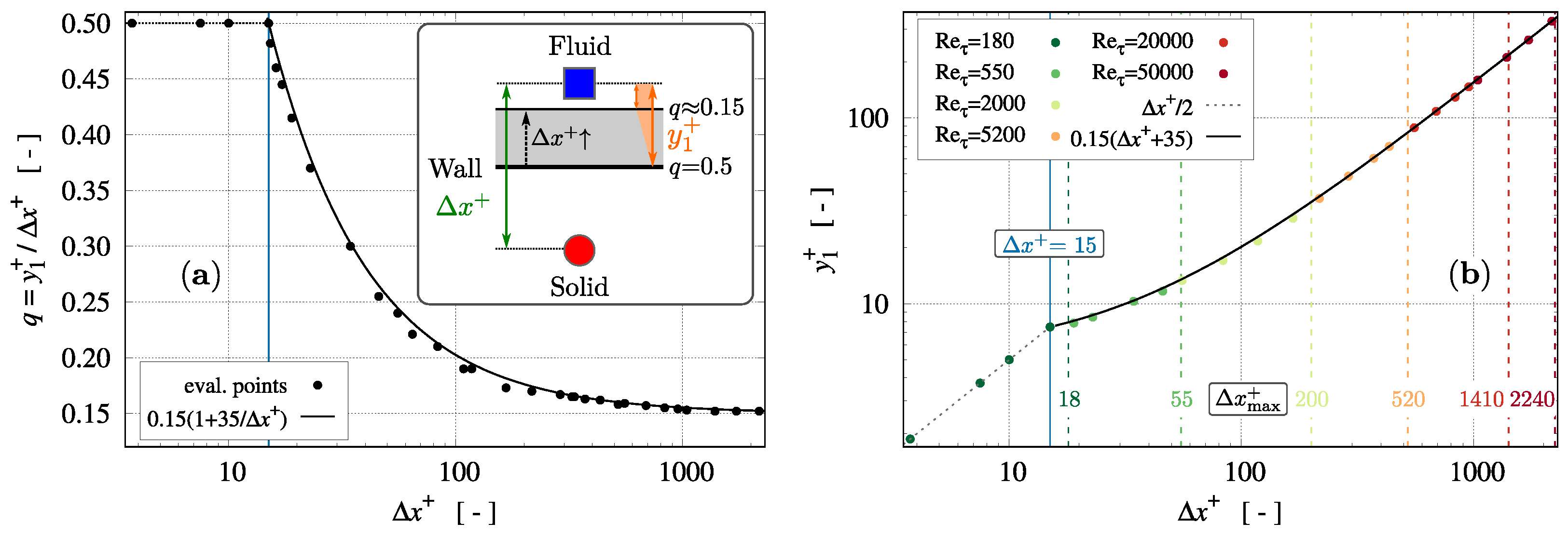
2.2. Test Case and Parameter Space

The dimensions of the investigated channel are $6\pi H$ in streamwise (x), $2\pi H$ in spanwise (z), and $2H$ in wall-normal direction (y), cf. Figure 2b. Six Reynolds numbers are employed to analyze the capabilities of the C-LBM, i.e., ${\mathrm{Re}}_{\tau }=\{$180, 550, 2000, 5200, 20,000, 50,000}. The investigations are performed on various grids. They are characterized by the resolution of the channel half height with $N_H$ nodes and support investigating a large range of non-dimensional resolutions, i.e., $4\lesssim \Delta x^{+}=\Delta x{u}_{\tau }/\nu \lesssim$ 2200. As indicated by

Table 1. Summary of the investigated grids and Reynolds numbers as well as their color codes used in the following mean velocity plots. $N_H$ denoting the number of discrete nodes per channel half height and (rounded) ${\mathrm{Re}}_B$ data correspond to Dean’s correlation (${\mathrm{Re}}_B\approx 7.32{\mathrm{Re}}_{\tau }^{8/7}$). Furthermore, the resulting non-dimensional grid spacings $\Delta x^{+}({\mathrm{Re}}_{\tau },N_H)$ are listed.

${\mathbf{Re}}_{\mathit{\tau }}$	180		550		2000		5200		20,000		50,000
${\mathbf{Re}}_{\mathit{B}}$	2800		9900		43,400		129,200		602,500		1,717,000
	${\mathit{N}}_{\mathit{H}}$	$\Delta {\mathit{x}}^{+}$	${\mathit{N}}_{\mathit{H}}$	$\Delta {\mathit{x}}^{+}$	${\mathit{N}}_{\mathit{H}}$	$\Delta {\mathit{x}}^{+}$	${\mathit{N}}_{\mathit{H}}$	$\Delta {\mathit{x}}^{+}$	${\mathit{N}}_{\mathit{H}}$	$\Delta {\mathit{x}}^{+}$	${\mathit{N}}_{\mathit{H}}$	$\Delta {\mathit{x}}^{+}$
■	48	3.8	29	19	36	56	24	220	36	555	48	1040
▲	24	7.5	24	23	24	83	18	290	29	690	36	1390
●	18	10	16	34	17	118	14	370	24	825	29	1740
◆	12	15	12	46	12	167	12	430	21	960	23	2170

, each Reynolds number is investigated on four grids that coarsen from dark green to red. The selected resolutions aim at an approximately equal change in $\Delta x^{+}$ while also considering resolutions of particular interest.

The Mach number is assigned to $\mathrm{Ma}=0.1$ in response to previous investigations [27,28]. Each simulation comprises 200 flow passes $T=6\pi H/u_B$ through the domain. An initial phase of 50 T is followed by a moving average computation of the mean flow and the contributions of the viscous and modeled stresses, which usually also span 50 T. Once the mean velocity is converged, the Reynolds stresses are evaluated during the final 100 T.

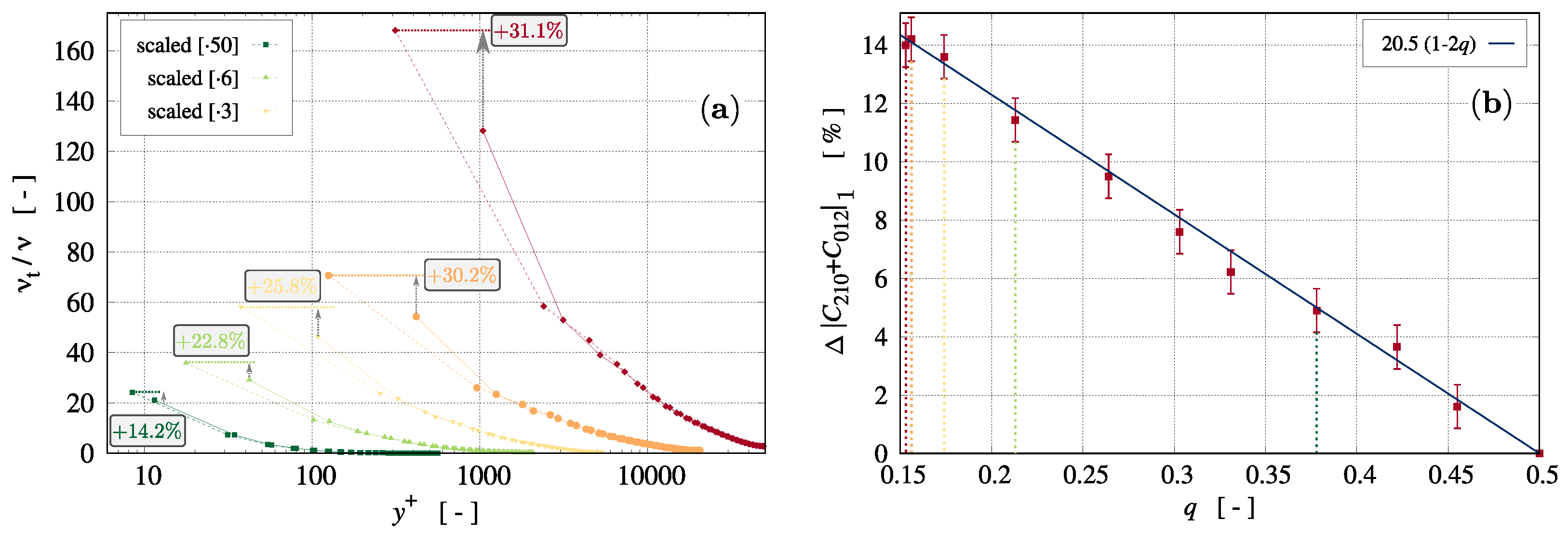
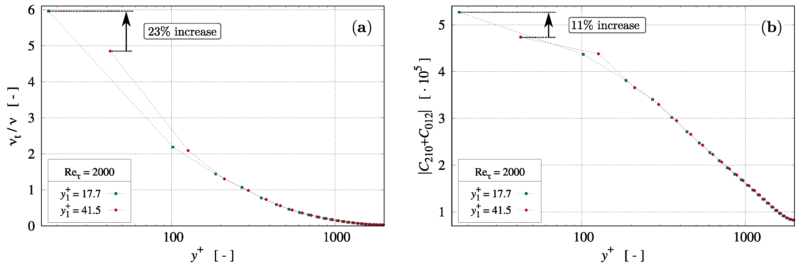
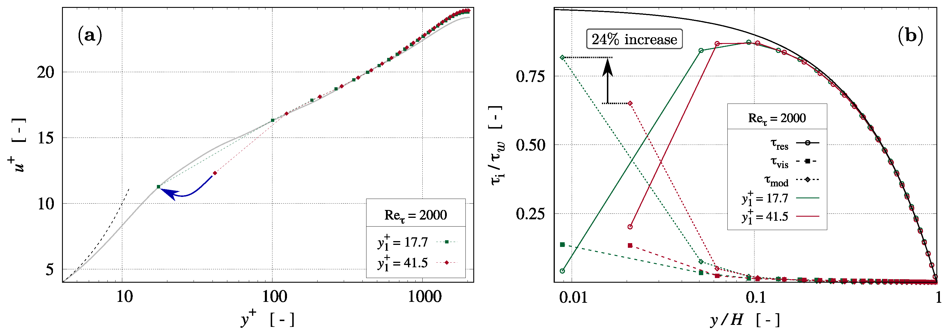
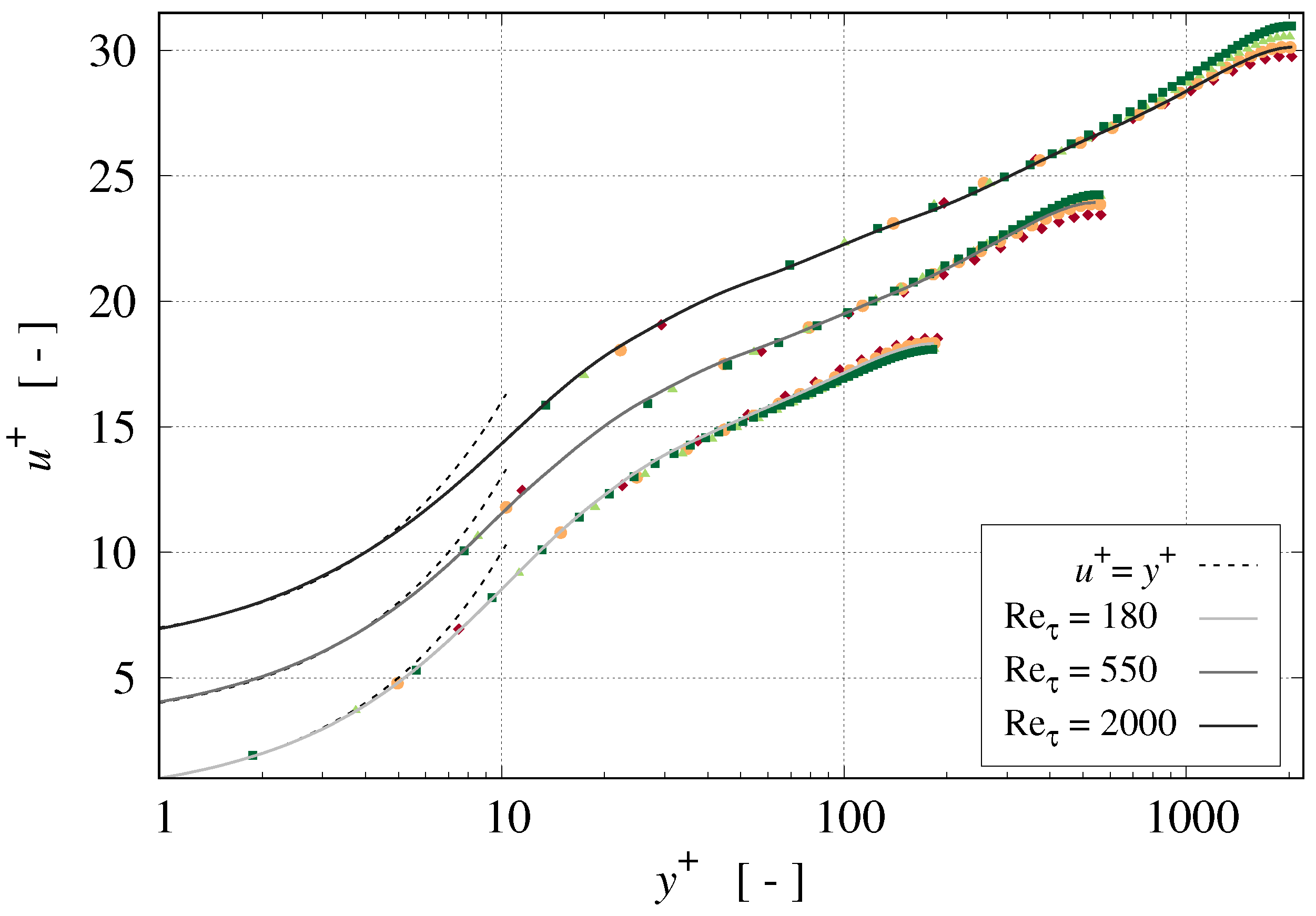
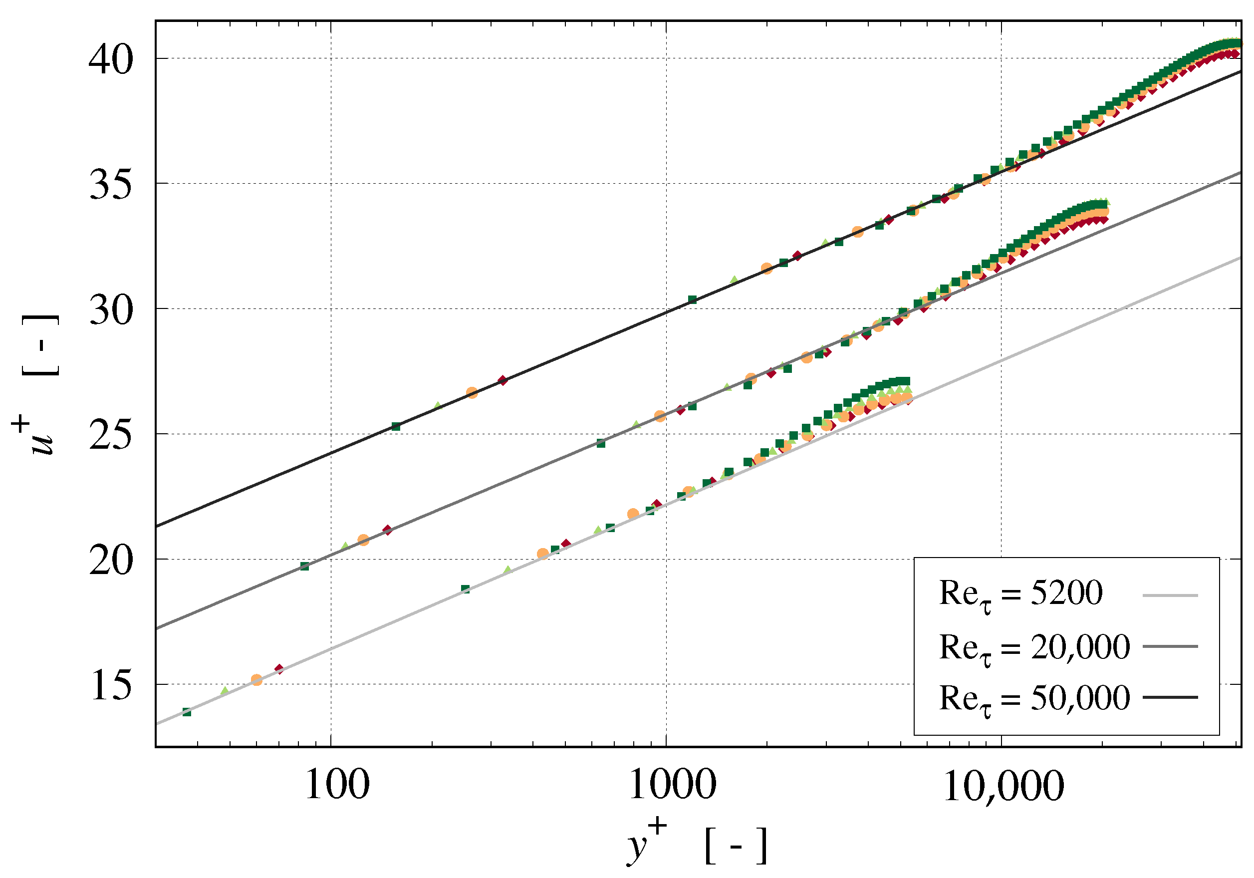
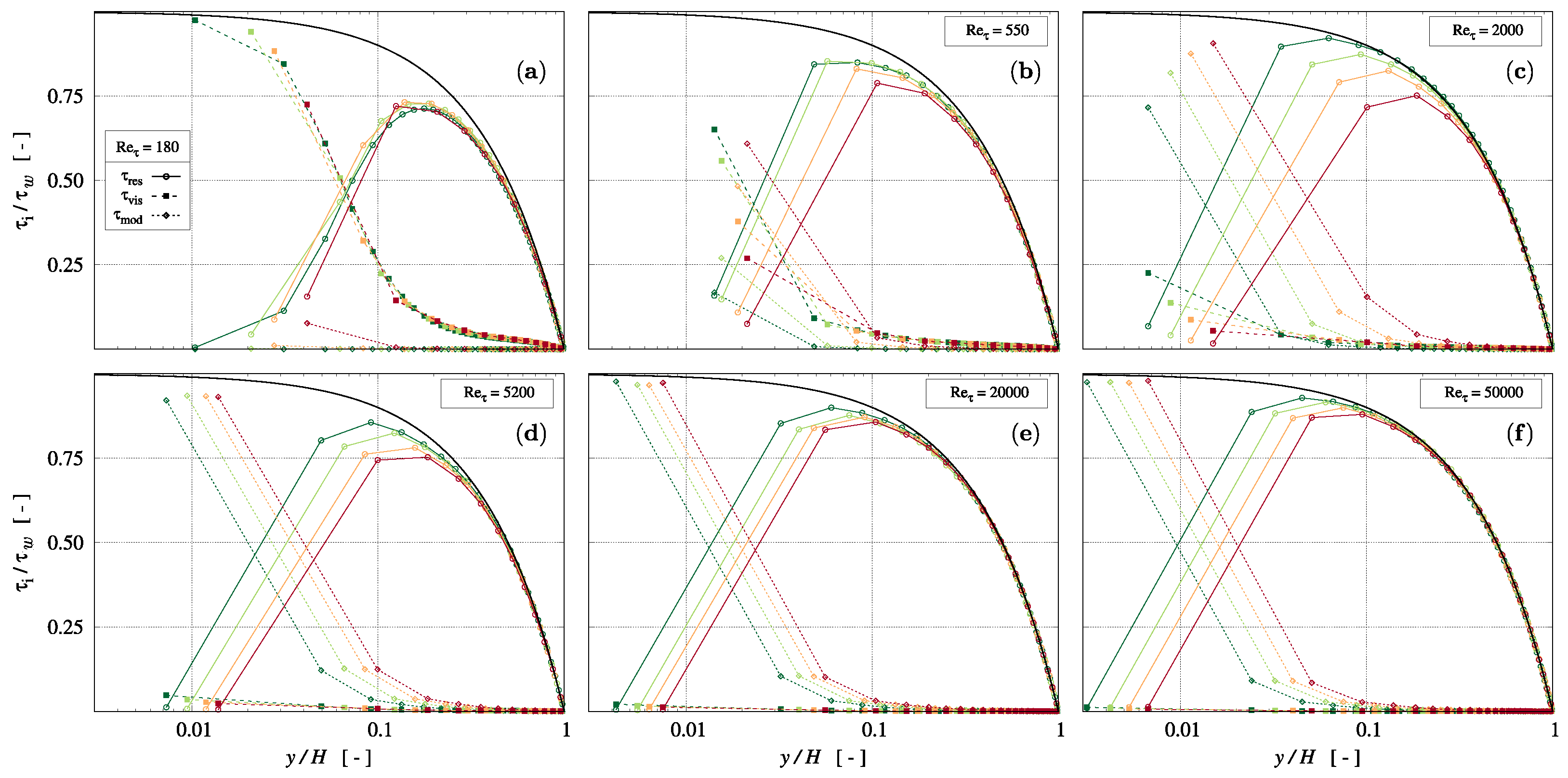
3. Results and Discussion

The present results represent a follow-up study of a recently published paper [27], where the regularized dynamic cumulant lattice Boltzmann (LES) method summarized in Section 2.1 was applied to simulate turbulent channel flows on a homogeneous, Cartesian lattice. As indicated by selected results shown in Figure 1, fair average velocities, Reynolds stresses, spectra, and correlation lengths are reported for ${\mathrm{Re}}_B\in$ [2800, 130,000] by the same LBM formulation in [27]. An exception refers to significant overestimated near-wall gradients observed for the higher Reynolds numbers, which might deteriorate the assessment of engineering quantities of importance, e.g., heat fluxes. The deficit is deemed to be related to the interaction of the wall function with the cumulant-based subgrid stress model. In conclusion, a simple correction is sought that alleviates these deficits.

To understand the rationale of the suggested correction, it is essential to note that the second fluid node serves as a reference location for constructing the wall function. The latter iteratively computes a consistent shear stress ${\tau }_w$ in line with the velocity prediction. Thus, the related (instantaneous) shear stress velocity $u_{\tau }=\sqrt{|{\tau }_w|/\rho }$) provides a valid $<y_2^{+},u_2^{+}>$ combination (with $y_i^{+}=y_i{u}_{\tau }/\nu$ and $u_i^{+}=u_i/u_{\tau }$) at the second fluid node for a given wall distance $y_2$ and a simulated (instantaneous) velocity $u_2$ at this node [27].

We suggest manipulating the non-dimensional wall distance of the first fluid node $y_1^{+}$ from its standard value of $y_1^{+}=\Delta x^{+}/2$ virtually, i.e., without changing the actual grid, cf. the sketch in Figure 3a. Since no deficits occur for an adequate resolution of the near-wall regime, no manipulation of the wall distance is needed for $\Delta x^{+}\le 15$. A comprehensive parameter study is performed for a wide range of Reynolds numbers ${\mathrm{Re}}_{\tau }\in$ [550, 50,000] to compile the appropriate wall location shift. As indicated by the symbols in Figure 3, a fair correlation for an adequate near-wall distance of the first fluid node reads

$$\begin{array}{c}\hfill y_1^{+}(\Delta x^{+})=\left\{\begin{array}{cc}0.5\Delta x^{+},\hfill & \Delta x^{+}\le 15\hfill \\ \left[0.15\right(1+35/\Delta x^{+})]\Delta x^{+},\hfill & \Delta x^{+}>15\hfill \end{array}\right..\end{array}$$

(10)

On the one hand, this virtual shift of the $y^{+}$-origin reduces the wall distance. On the other hand, the relative reduction decreases with increasing distance, and the manipulation substantially shifts the wall distance of the first fluid node to the left. At the same time, the reduced distance increases the third-order cumulant expression at the first fluid node inside the Smagorinsky parameter ${\mathcal{C}}_{\mathrm{S}}$ (9) roughly linearly for high Reynolds number flows, cf. Figure 4b and the derivation of the regularization term in [27].

This yields an increase in the eddy viscosity ${\nu }_t={\mathcal{C}}_s^2{\Delta }^{2}S$ that approximately scales with ${\mathcal{C}}_{\mathrm{S}}^2$, as indicated by Figure 4a and Figure 5a.

As indicated by cf. Figure 6a, the velocity gradient between the solid node and the reference second fluid node, i.e., the centered velocity gradient at the first fluid node, does virtually not change. The latter is easily understood by the example given in Figure 5 and Figure 6, where $|{\tau }_{\mathrm{mod}}|={\nu }_{t}S={\mathcal{C}}_{\mathrm{S}}^2{\Delta }^2{S}^2$ increases by 24% in response to a 23% increase in the eddy viscosity and an 11% augmentation of ${\mathcal{C}}_{\mathrm{S}}$. The unaltered strain rate at the first fluid node is crucial to control the modeled stress by the exclusive change in the third-order cumulant expression $|C_{210}+C_{012}{|}_1$ at the first fluid node in response to the shift in the wall location, while leaving the grid and the numerical approach unchanged.

It is also interesting to note that the influence of the suggested wall positioning modification is almost exclusively restricted to the computed eddy viscosity (and the cumulants) at the first fluid node, cf. Figure 4a, and therefore can be interpreted as a local adjustment of the subgrid scale model to the wall function.

Figure 7 and Figure 8 display the predicted non-dimensional mean velocity profiles of the three lower and higher Reynolds numbers, respectively. All results are obtained with the adjustment of the wall location according to Equation (10).

Since all wall-adjacent nodes are located above the buffer-layer for the higher Reynolds numbers displayed in Figure 8, the lower bound of the abscissa is set to $y_1^{+}=30$ in order to emphasize the logarithmic layer and the wake flow. The characteristic of the logarithmic layer is in fair predictive agreement with the parameters found by Nikitin et al. [55] for turbulent channel flows up to ${\mathrm{Re}}_{\tau }=$ 80,000 ($\kappa =0.41$ and $B=5.2$).

Further analysis of the mean flow profiles reveals a sensitivity of the present C-LBM to predict wake flows [56] depending on the resolution. In line with previous LES or DES simulations, e.g., those of Cabot et al. [57] or Keating and Piomelli [58], the present C-LBM also portrays an attenuation of the wake flow when the resolution is coarsened. This is caused by a weaker reduction in the resolved stresses in the outer regime of the boundary layer, as illustrated in Figure 9.

Mind that wake flow usually occurs beyond a critical Reynolds number, e.g., ${\mathrm{Re}}_{\tau }\ge 1000$ [59], and hence no substantial grid sensitivity is observed for the two lower Reynolds numbers in Figure 7, and no significant change in the reduction in resolved stress towards the exterior boundary layer region is displayed in Figure 9a,b when the grid is coarsened. The analysis of the wake prediction yields a heuristic criterion for the maximum grid coarseness through

$$\begin{array}{c}\hfill \Delta x_{\max }^{+}\left({\mathrm{Re}}_{\tau }\right)=\left\{\begin{array}{cc}{\mathrm{Re}}_{\tau }/10,\hfill & {\mathrm{Re}}_{\tau }\lesssim {10}^4\left(\mathrm{to}\mathrm{capture}\mathrm{wake}\right)\hfill \\ 10\sqrt{{\mathrm{Re}}_{\tau }},\hfill & {\mathrm{Re}}_{\tau }>{10}^4\left(\mathrm{to}\mathrm{capture}\mathrm{wake}\mathrm{and}\mathrm{maintain}\mathrm{the}\mathrm{validity}\mathrm{of}\right(10\left)\right)\hfill \end{array}\right..\end{array}$$

(11)

For the investigated Reynolds numbers ${\mathrm{Re}}_{\tau }=\{$180, 550, 2000, 5200, 20,000, 50,000}, the coarsest resolutions derived from Equation (11) read $\Delta x_{\max }^{+}\left({\mathrm{Re}}_{\tau }\right)=\{$18, 55, 200, 520, 1410, 2240}, which are close to the coarsest (◆) investigated grids in Table 1.

4. Conclusions

The paper scrutinizes the predictive performance of a D3Q27 cumulant-based LB method to capture turbulent channel flows. Emphasis is given to assessing a unified computational model utilizing adaptive, dynamic regularization and subgrid scale components based on cumulant expressions combined with a universal wall treatment. The approach aims at resolution independence and is based on a previously published suggestion of the authors [27]. The essential building blocks and main advantages of this strategy are (a) an alternative regularization that dissipates the kinetic energy of the large wave numbers and accurately computes flows with fine to moderate resolutions ($\Delta x^{+}\lesssim 20$) and (b) a third-order cumulant expression to formulate a dynamic Smagorinsky-type SGS model that acts on smaller wave numbers. Both elements are sensitized to the resolution through the cell Reynolds (spatial) and Mach numbers (temporal) and seamlessly vanish in the fine-grid limit.

A remaining deficit refers to overshoot issues due to the missing interplay between the wall function and the SGS model nearby the wall. Related misinterpretations of the averaged flow field might yield a substantially wrong prediction of the wall shear stress and heat transfer rate at higher Reynolds numbers of engineering interest. Depending on the local flow situation, the modeled shear stress contributions are up to 30% wrong in response to the overshoot phenomenon. The problem is particularly prominent for $\Delta x_1^{+}\gtrsim 20$. The present paper proposes an adjustment of a universal wall function that comes at negligible computational expenses and favorably influences the near-wall cumulant expressions.

To render the predictive benefits, attention is devoted to a comprehensive range of bulk Reynolds numbers ${\mathrm{Re}}_B\in [3000,1.7\times {10}^6]$ on grids between $4.5\times {10}^5$ and $27\times {10}^6$ nodes that feature resolutions of $\Delta x^{+}\in [4,2200]$. The results indicate that the unified model is able to capture all investigated flows without further adjustments or user input. Future research could consider implementing the approach for complex geometries to predict separated engineering shear flows.

References

1. Spalding, D. A single formula for the law of wall. J. Appl. Mech. 1961, 28, 455–458. [Google Scholar] [CrossRef]
2. Grotjans, H.; Menter, F. Wall Functions for General Application CFD Codes. In Computational Fluid Dynamics ’98, Proceedings of the 4th European Computational Fluid Dynamics Conference, Athens, Greece, 7–11 September 1998; Papailiou, K., Tsahalis, D., Periaux, J., Hirsch, C., Pandolfi, M., Eds.; John Wiley & Sons: Chichester, UK, 1998; pp. 1112–1117. [Google Scholar]
3. Rung, T.; Lübcke, H.; Thiele, F. Universal wall-boundary conditions for turbulence-transport models. ZAMM J. Appl. Math. Mech. Z. Für Angew. Math. Und Mech. 2001, 81, 481–482. [Google Scholar] [CrossRef]
4. Spalart, P.; Jou, W.H.; Strelets, M.; Allmaras, S.; Liu, C.; Liu, Z.; Sakell, L. Comments on the Feasibility of LES for Wings, and on a Hybrid RANS/LES Approach. In Proceedings of the First AFOSR International Conference on DNS/LES: Direct numerical simulation and large eddy simulation, Ruston, LA, USA, 4–8 August 1997; Greyden Press: Dayton, OH, USA, 1997; pp. 137–148. [Google Scholar]
5. Travin, A.; Shur, M.; Strelets, M.; Spalart, P. Detached-Eddy Simulations Past a Circular Cylinder. Flow Turbul. Combust. 2000, 63, 293–313. [Google Scholar] [CrossRef]
6. Spalart, P.; Deck, S.; Shur, M.; Squires, K.; Strelets, M.; Travin, A. A New Version of Detached-eddy Simulation, Resistant to Ambiguous Grid Densities. Theor. Comput. Fluid Dyn. 2006, 20, 181. [Google Scholar] [CrossRef]
7. Shur, M.; Spalart, P.; Strelets, M.; Travin, A. A hybrid RANS-LES model with delayed DES and wall-modeled LES capabilities. Int. J. Heat Fluid Flow 2008, 29, 1638–1649. [Google Scholar] [CrossRef]
8. Gritskevich, M.; Garbaruk, A.; Schütze, J.; Menter, F. Development of DDES and IDDES Formulations for the k-ω Shear Stress Transport Model. Flow Turbul. Combust. 2012, 88, 431–449. [Google Scholar] [CrossRef]
9. Kotapati, R.; Keatin, A.; Kandasamy, S.; Duncan, B.; Shock, R.; Chen, H. The Lattice-Boltzmann-VLES Method for Automotive Fluid Dynamics Simulation, a Review; Technical Report 2009-26-0057; SAE International: Warrendale, PA, USA, 2009. [Google Scholar] [CrossRef]
10. Noelting, S.; Fares, E. The Lattice-Boltzmann Method: An Alternative to LES for Complex Aerodynamic and Aeroacoustic Simulations in the Aerospace Industry; Technical Report 2015-01-2575; SAE International: Warrendale, PA, USA, 2015. [Google Scholar] [CrossRef]
11. Niedermeier, C.; Janßen, C.; Indinger, T. Massively-parallel multi-GPU simulations for fast and accurate automotive aerodynamics. In Proceedings of the 7th European Conference on Computational Fluid Dynamics, Glasgow, Scotland, UK, 11–15 June 2018. [Google Scholar]
12. Lenz, S.; Schönherr, M.; Geier, M.; Krafczyk, M.; Pasquali, A.; Christen, A.; Giometto, M. Towards real-time simulation of turbulent air flow over a resolved urban canopy using the cumulant lattice Boltzmann method on a GPGPU. J. Wind Eng. Ind. Aerodyn. 2019, 189, 151–162. [Google Scholar] [CrossRef]
13. Sharma, K.; Straka, R.; Tavares, F. Lattice Boltzmann Methods for Industrial Applications. Ind. Eng. Chem. Res. 2019, 58, 16205–16234. [Google Scholar] [CrossRef]
14. Krüger, T.; Kusumaatmaja, H.; Kuzmin, A.; Shardt, O.; Silva, A.; Viggen, E. The Lattice Boltzmann Method; Springer International Publishing: Cham, Switzerland, 2017. [Google Scholar]
15. Janßen, C.; Mierke, D.; Überrück, M.; Gralher, S.; Rung, T. Validation of the GPU-Accelerated CFD Solver ELBE for Free Surface Flow Problems in Civil and Environmental Engineering. Computation 2015, 3, 354–385. [Google Scholar] [CrossRef]
16. Geier, M.; Schönherr, M.; Pasquali, A.; Krafczyk, M. The cumulant lattice Boltzmann equation in three dimensions: Theory and validation. Comput. Math. Appl. 2015, 70, 507–547. [Google Scholar] [CrossRef]
17. Schornbaum, F.; Rüde, U. Massively parallel algorithms for the Lattice Boltzmann Method on nonuniform grids. SIAM J. Sci. Comput. 2016, 38, 96–126. [Google Scholar] [CrossRef]
18. Watanabe, S.; Aoki, T. Large-scale flow simulations using lattice Boltzmann method with AMR following free-surface on multiple GPUs. Comput. Phys. Commun. 2021, 264, 107871. [Google Scholar] [CrossRef]
19. Latt, J.; Malaspinas, O.; Kontaxakis, D.; Parmigiani, A.; Lagrava, D.; Brogi, F.; Belgacem, M.; Thorimbert, Y.; Leclaire, S.; Li, S.; et al. Palabos: Parallel Lattice Boltzmann Solver. Comput. Math. Appl. 2021, 81, 334–350. [Google Scholar] [CrossRef]
20. Feng, Y.; Miranda-Fuentes, J.; Guo, S.; Jacob, J.; Sagaut, P. ProLB: A Lattice Boltzmann Solver of Large-Eddy Simulation for Atmospheric Boundary Layer Flows. J. Adv. Model. Earth Syst. 2021, 13, e2020MS002107. [Google Scholar] [CrossRef]
21. Coreixas, C.; Wissocq, G.; Chopard, B.; Latt, J. Impact of collision models on the physical properties and the stability of lattice Boltzmann methods. Philos. Trans. R. Soc. A 2020, 378, 20190397. [Google Scholar] [CrossRef]
22. Geier, M.; Pasquali, A.; Schönherr, M. Parametrization of the cumulant lattice Boltzmann method for fourth order accurate diffusion part I: Derivation and validation. J. Comput. Phys. 2017, 348, 862–888. [Google Scholar] [CrossRef]
23. Geier, M.; Lenz, S.; Schönherr, M.; Krafczyk, M. Under-resolved and large eddy simulations of a decaying Taylor-Green vortex with the cumulant lattice Boltzmann method. Theor. Comput. Fluid Dyn. 2021, 35, 169–208. [Google Scholar] [CrossRef]
24. Gruszczyński, G.; Łaniewski Wołłk, L. A comparative study of 3D cumulant and central moments lattice Boltzmann schemes with interpolated boundary conditions for the simulation of thermal flows in high Prandtl number regime. Int. J. Heat Mass Transf. 2022, 197, 123259. [Google Scholar] [CrossRef]
25. Sato, K.; Kawasaki, K.; Koshimura, S. A comparative study of the cumulant lattice Boltzmann method in a single-phase free-surface model of violent flows. Comput. Fluids 2022, 236, 105303. [Google Scholar] [CrossRef]
26. Gehrke, M.; Banari, A.; Rung, T. Performance of Under-Resolved, Model-Free LBM Simulations in Turbulent Shear Flows. In Progress in Hybrid RANS-LES Modelling; Notes on Numerical Fluid Mechanics and Multidisciplinary Design; Hoarau, Y., Peng, S.H., Schwamborn, D., Revell, A., Mockett, C., Eds.; Springer International Publishing: Cham, Switzerland, 2020; Volume 143, pp. 3–18. [Google Scholar] [CrossRef]
27. Gehrke, M.; Rung, T. Scale-resolving turbulent channel flow simulations using a dynamic cumulant lattice Boltzmann method. Phys. Fluids 2022, 34, 075129. [Google Scholar] [CrossRef]
28. Gehrke, M.; Rung, T. Periodic hill flow simulations with a parameterized cumulant lattice Boltzmann method. Int. J. Numer. Methods Fluids 2022, 94, 1111–1154. [Google Scholar] [CrossRef]
29. Asmuth, H.; Janßen, C.; Olivares-Espinosa, H.; Ivanell, S. Wall-modeled lattice Boltzmann large-eddy simulation of neutral atmospheric boundary layers. Phys. Fluids 2021, 33, 105111. [Google Scholar] [CrossRef]
30. Yu, D.; Mei, R.; Shyy, W. A Unified Boundary Treatment in Lattice Boltzmann Method. In Proceedings of the 41st Aerospace Sciences Meeting and Exhibit, Reno, NV, USA, 6–9 January 2003; AIAA 2003–0953. American Institute of Aeronautics and Astronautics: Reston, VA, USA, 2003. [Google Scholar] [CrossRef]
31. Kim, J.; Moin, P.; Moser, R. Turbulence statistics in fully developed channel flow at low Reynolds number. J. Fluid Mech. 1987, 177, 133–166. [Google Scholar] [CrossRef]
32. Bernardini, M.; Pirozzoli, S.; Orlandi, P. Velocity statistics in turbulent channel flow up to Reτ = 4000. J. Fluid Mech. 2014, 742, 171–191. [Google Scholar] [CrossRef]
33. Brasseur, J.; Wei, T. Designing large-eddy simulation of the turbulent boundary layer to capture law-of-the-wall scaling. Phys. Fluids 2010, 22, 021303. [Google Scholar] [CrossRef]
34. Haussmann, M.; Claro Barreto, A.; Lipeme Kouyi, G.; Rivière, N.; Nirschl, H.; Krause, M. Large-eddy simulation coupled with wall models for turbulent channel flows at high Reynolds numbers with a lattice Boltzmann method—Application to Coriolis mass flowmeter. Comput. Math. Appl. 2019, 78, 3285–3302. [Google Scholar] [CrossRef]
35. Pasquali, A.; Geier, M.; Krafczyk, M. Near-wall treatment for the simulation of turbulent flow by the cumulant lattice Boltzmann method. Comput. Math. Appl. 2020, 79, 195–212. [Google Scholar] [CrossRef]
36. Han, M.; Ooka, R.; Kikumoto, H. A wall function approach in lattice Boltzmann method: Algorithm and validation using turbulent channel flow. Fluid Dyn. Res. 2021, 53, 045506. [Google Scholar] [CrossRef]
37. Degrigny, J.; Cai, S.H.; Boussuge, J.F.; Sagaut, P. Improved wall model treatment for aerodynamic flows in LBM. Comput. Fluids 2021, 227, 105041. [Google Scholar] [CrossRef]
38. Gehrke, M.; Janßen, C.; Rung, T. Scrutinizing lattice Boltzmann methods for direct numerical simulations of turbulent channel flows. Comput. Fluids 2017, 156, 247–263. [Google Scholar] [CrossRef]
39. Banari, A.; Gehrke, M.; Janßen, C.; Rung, T. Numerical simulation of nonlinear interactions in a naturally transitional flat plate boundary layer. Comput. Fluids 2020, 203, 104502. [Google Scholar] [CrossRef]
40. Chen, S.; Doolen, G. Lattice Boltzmann method for fluid flows. Annu. Rev. Fluid Mech. 1998, 30, 329–364. [Google Scholar] [CrossRef]
41. Succi, S. The Lattice Boltzmann Equation for Fluid Dynamics and Beyond; Clarendon Press: Cary, NC, USA, 2001. [Google Scholar]
42. Yu, D.; Mei, R.; Luo, L.S.; Shyy, W. Viscous flow computations with the method of lattice Boltzmann equation. Prog. Aerosp. Sci. 2003, 39, 329–367. [Google Scholar] [CrossRef]
43. Mohamad, A. Lattice Boltzmann Method; Springer: London, UK, 2011. [Google Scholar]
44. Qian, Y.; d’Humières, D.; Lallemand, P. Lattice BGK Models for Navier Stokes Equation. Europhys. Lett. 1992, 17, 479–484. [Google Scholar] [CrossRef]
45. He, X.; Luo, L.S. Theory of the lattice Boltzmann method: From the Boltzmann equation to the lattice Boltzmann equation. Phys. Rev. E 1997, 56, 6811–6817. [Google Scholar] [CrossRef]
46. Dubief, Y.; Delcayre, F. On coherent-vortex identification in turbulence. J. Turbul. 2000, 1, N11. [Google Scholar] [CrossRef]
47. Dean, R. Reynolds number dependence of skin friction and other bulk flow variables in two-dimensional rectangular duct flow. J. Fluids Eng. 1978, 100, 215–223. [Google Scholar] [CrossRef]
48. Bhatnagar, P.; Gross, E.; Krook, M. A Model for Collision Processes in Gases. I. Small Amplitude Processes in Charged and Neutral One-Component Systems. Phys. Rev. 1954, 94, 511–525. [Google Scholar] [CrossRef]
49. Ginzburg, I.; Verhaeghe, F.; d’Humières, D. Two-Relaxation-Time Lattice Boltzmann Scheme: About Parametrization, Velocity, Pressure and Mixed Boundary Conditions. Commun. Comput. Phys. 2008, 3, 427–478. [Google Scholar]
50. D’Humières, D.; Ginzburg, I.; Krafczyk, M.; Lallemand, P.; Luo, L.S. Multiple-relaxation-time lattice Boltzmann models in three dimensions. Philos. Trans. R. Soc. A 2002, 360, 437–451. [Google Scholar] [CrossRef]
51. Tölke, J.; Freudiger, S.; Krafczyk, M. An adaptive scheme using hierarchical grids for lattice Boltzmann multi-phase flow simulations. Comput. Fluids 2006, 35, 820–830. [Google Scholar] [CrossRef]
52. Bösch, F.; Chikatamarla, S.; Karlin, I. Entropic multirelaxation lattice Boltzmann models for turbulent flows. Phys. Rev. E 2015, 92, 043309. [Google Scholar] [CrossRef] [PubMed]
53. Seeger, S.; Hoffmann, K. The cumulant method for computational kinetic theory. Contin. Mech. Thermodyn. 2000, 12, 403–421. [Google Scholar] [CrossRef]
54. Smagorinsky, J. General Circulation Experiments with the Primitive Equations. Mon. Weather Rev. 1963, 91, 99–164. [Google Scholar] [CrossRef]
55. Nikitin, N.; Nicoud, F.; Wasistho, B.; Squires, K.; Spalart, P. An approach to wall modeling in large-eddy simulations. Phys. Fluids 2000, 12, 1629–1632. [Google Scholar] [CrossRef]
56. Coles, D. The law of the wake in the turbulent boundary layer. J. Fluid Mech. 1956, 1, 191–226. [Google Scholar] [CrossRef]
57. Cabot, W.; Jiménez, J.; Baggett, J. On wakes and near-wall behavior in coarse large-eddy simulation of channel flow with wall models and second-order finite-difference methods. In Annual Research Briefs; Center for Turbulence Research, NASA/Stanford University: Stanford, CA, USA, 1999; pp. 343–354. [Google Scholar]
58. Keating, A.; Piomelli, U. A dynamic stochastic forcing method as a wall-layer model for large-eddy simulation. J. Turbul. 2006, 7, N12. [Google Scholar] [CrossRef]
59. Schultz, M.; Flack, K. Reynolds-number scaling of turbulent channel flow. Phys. Fluids 2013, 25, 025104. [Google Scholar] [CrossRef] [Green Version]
Figure 1. (a) Comparison of predicted non-dimensional mean velocity profiles u + = u / u τ as functions of the non-dimensional distance y + = y u τ / ν returned by the modified C-LBM for N H = 24 along the channel half height (symbols), the DNS data of Kim et al. [31] ( Re τ = 180 ) and the DNS data of Bernardini et al. [32] ( Re τ = 2000), indicated by solid lines. To improve the presentation, the mean velocity profile for Re τ = 2000 is shifted by Δ u + = 5 velocity units in vertical direction. (b) Evolution of (averaged) resolved (solid/circles), viscous (dashed/squares), modeled (dotted/diamonds), and total (black line) normalized shear stress contributions.
Computation 10 00171 g001
Figure 2. (a) Illustration of the employed D3Q27 discretization. (b) Dimensions of the investigated channel flow featuring isosurface snapshots of the Q-criterion [46], colored by the streamwise (x-direction) velocity component for Re B 1.7 × 10 6 on a homogeneous Cartesian grid featuring approximately 27 million lattice nodes ( H / Λ H = N H = 48 ).
Computation 10 00171 g002
Figure 3. Evolution of the suggested non-dimensional wall distance of the wall-adjacent fluid node y 1 + in normalized (a) and non-normalized (b) format, depending on the grid resolution Δ x + as described in Equation (10). Colored dots display evaluated discrete y 1 + optima of each Reynolds number and grid. Furthermore, the reasonable maximum resolution for each of the underlying Reynolds numbers is illustrated by colored dashed vertical lines.
Computation 10 00171 g003
Figure 4. (a) Comparison of the normalized predicted (averaged) eddy viscosity obtained from a centered wall location ( q = 0.5 ; solid lines) and an adjusted wall location (dotted lines) for Re τ = { 550, 2000, 5200, 20,000, 50,000} on the N H = 24 grid. (b) Increase in the (averaged) cumulant expression | C 210 + C 012 | 1 at the first fluid node as a function of the wall location parameter q = y 1 + / Δ x + . Error bars refer to Δ | C 210 + C 012 | 1 ± 0.75 % . Colored verticals correspond to the modified q-values on the N H = 24 grid in (a), whereas further data points refer to Re τ = 550 simulations employing N H = { 12 , 16 , 19 , 29 , 32 } from left to right.
Computation 10 00171 g004
Figure 5. (a) Increase in the normalized (averaged) eddy viscosity and (b) the related (averaged) cumulant expression at the first fluid node in response to a shift in the wall position computed from Equation (10) for Re τ = 2000 and Δ x + = 83 ( N H = 24 ).
Computation 10 00171 g005
Figure 6. (a) Non-dimensional mean velocity profiles for Re τ = 2000 on a grid featuring N H = 24 and Δ x + = 83 . The red velocity graph coincides with the red graph in Figure 1a and refers to the standard grid layout with y 1 + ( Δ x + ) = 0.5 Δ x + y 1 + ( Δ x + , Re τ ) . The green curve depicts results from the suggested y 1 + ( Δ x + , Re τ ) = 0.15 Δ x + ( 1 + 35 / Δ x + ) manipulation, cf. Equation (10). (b) The overshoot vanishes when the modeled shear stress increases due to an increase in the eddy viscosity, as displayed by the normalized (averaged) τ i partition pathlines.
Computation 10 00171 g006
Figure 7. Non-dimensional mean velocity profiles for three lower Reynolds numbers. Solid lines refer to reconstructions of discrete reference data sets published by Kim et al. [31] for Re τ = 180 and Bernardini et al. [32] for Re τ = { 550, 2000} as given in Gehrke and Rung [27]. The color codes of the symbols are given in Table 1. To improve the comparison, the profile for Re τ = 550 [ 2000 ] is vertically shifted by Δ u + = 3 [ 6 ] .
Computation 10 00171 g007
Figure 8. Non-dimensional mean velocity profiles for the three higher Reynolds numbers. With ascending Re τ the characteristic parameters of the logarithmic layer u + ( y + ) = ln ( y + ) / κ + B are: the von Kármán constant reads κ ( Re τ ) = { 0.40 , 0.41 , 0.41 } and the constants are B ( Re τ ) = { 4.9 , 4.9 , 5.0 } . The color codes of the symbols are given in Table 1. To improve the comparison, profiles for Re τ = 20,000 [50,000] are vertically shifted by Δ u + = 4 [ 8 ] .
Computation 10 00171 g008
Figure 9. (af) Comparison of (averaged) non-dimensional resolved (solid/circles), viscous (dashed/squares), and modeled (dotted/diamonds) shear stress contributions extended by the linear total stress relation τ tot / τ w = 1 y / H (solid black line) for all six investigated Re τ with four grids each.
Computation 10 00171 g009