Source Cell-Phone Identification in the Presence of Additive Noise from CQT Domain

Abstract
:1. Introduction
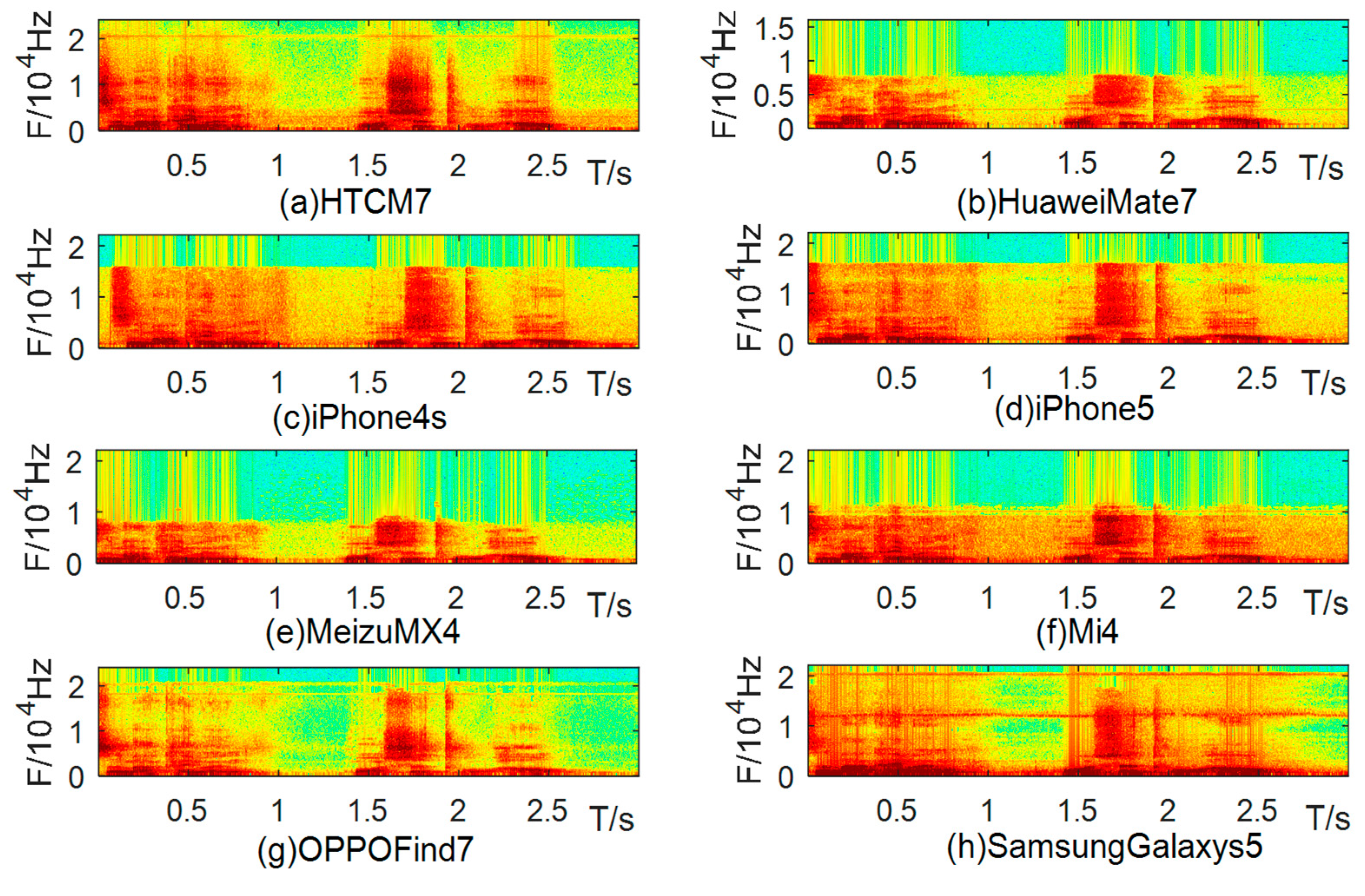
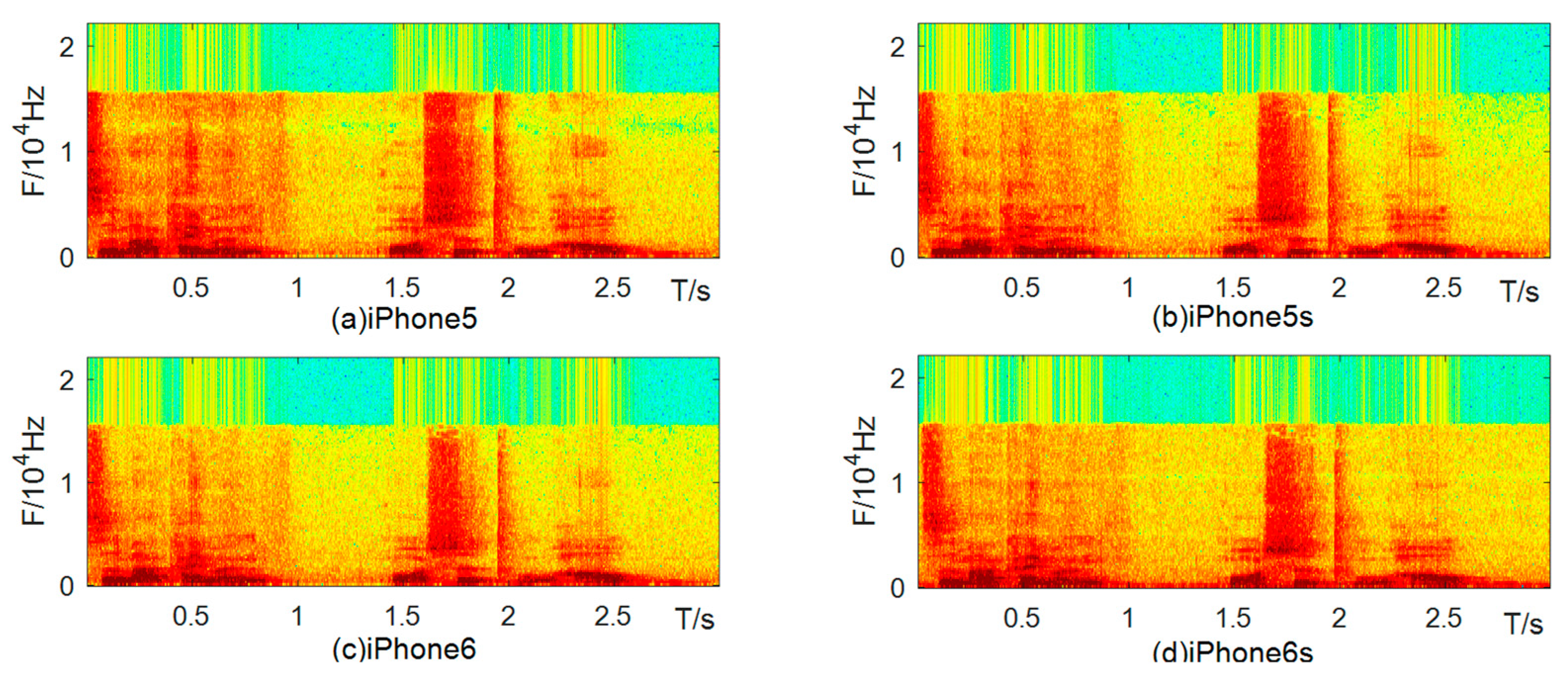
2. Device Difference Analysis
3. Feature Extraction
3.1. Spectral Distribution Features of the CQT Domain
- (1)
- If the time domain signal of a speech files is , and the frequency domain signal after the CQT is , is defined by:where k = 1, 2, ..., K is the frequency bin index; is the sampling rate; is the center frequency of bin k, which is exponentially distributed and is defined aswhere B is the number of bins per octave, is the center frequency of the lowest frequency bin and is computed according to:is a window function (Hanning window); from high frequency to low frequency, with the increasing frequency resolution, the time resolution will gradually be sacrificed. Therefore, the window length varies with k and is inversely proportional to k, namely:The Q-factor is a constant independent of k and is defined as the ratio of the center frequency to the bandwidth: .
- (2)
- For the frequency value of the i-th frame at the kth frequency point, the amplitude of is computed as follows:
- (3)
- Spectral distribution features:where represents the total number of frames of the speech in the kth frequency band, k = 1, 2, …, K. Therefore, for a speech file, its spectral distribution features comprise a 1 × K vector. K is set as 420 in this paper.
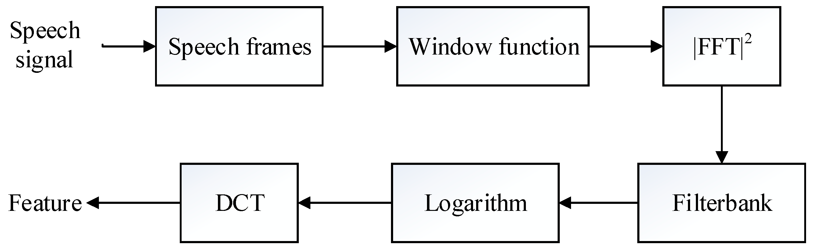
3.2. Traditional Features (MFCC, LFCC)
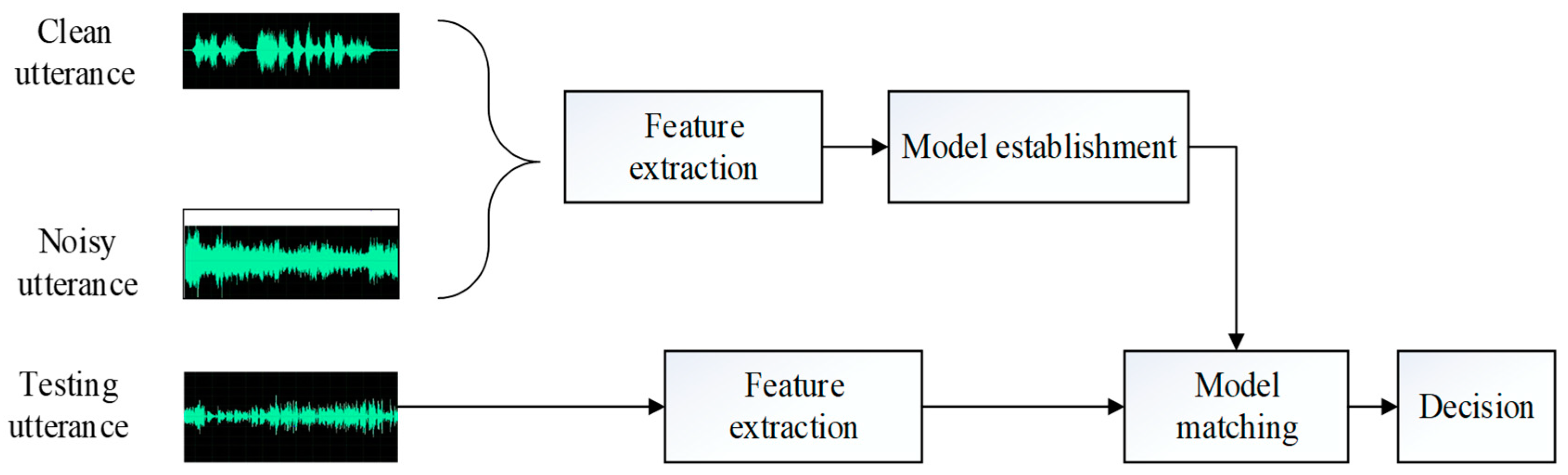
4. Classifiers and Algorithm Introduction
4.1. SVM
4.2. RF
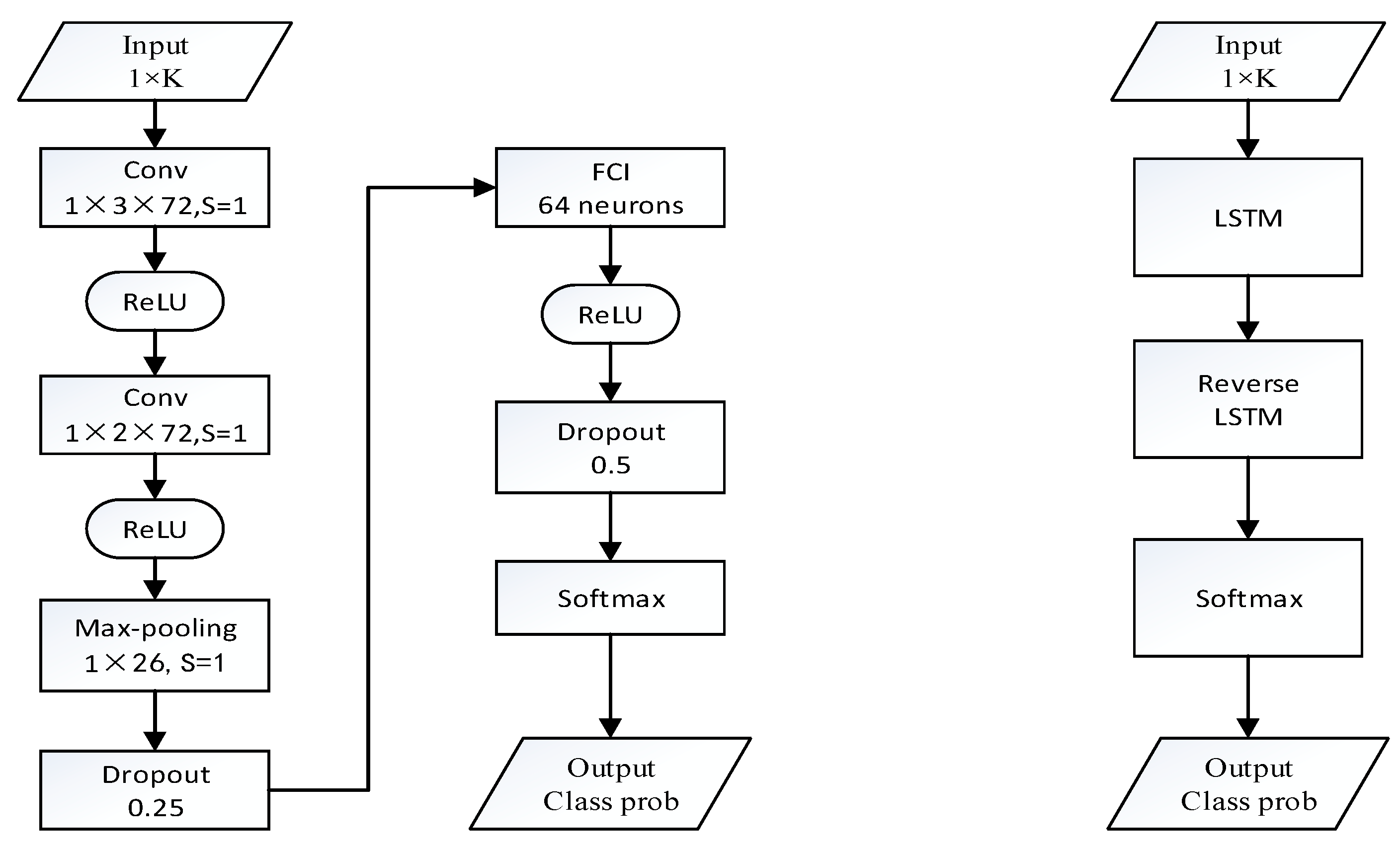
4.3. CNN
4.4. RNN-BLSTM
4.5. Multi-Scene Training Recognition Systems
5. Databases Construction
5.1. Basic Speech Databases
5.2. Noisy Speech Databases
6. Experiments
6.1. Experimental Setup
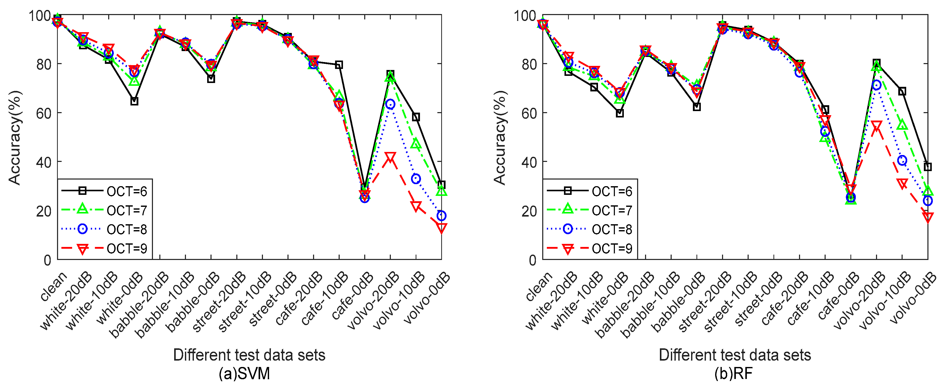
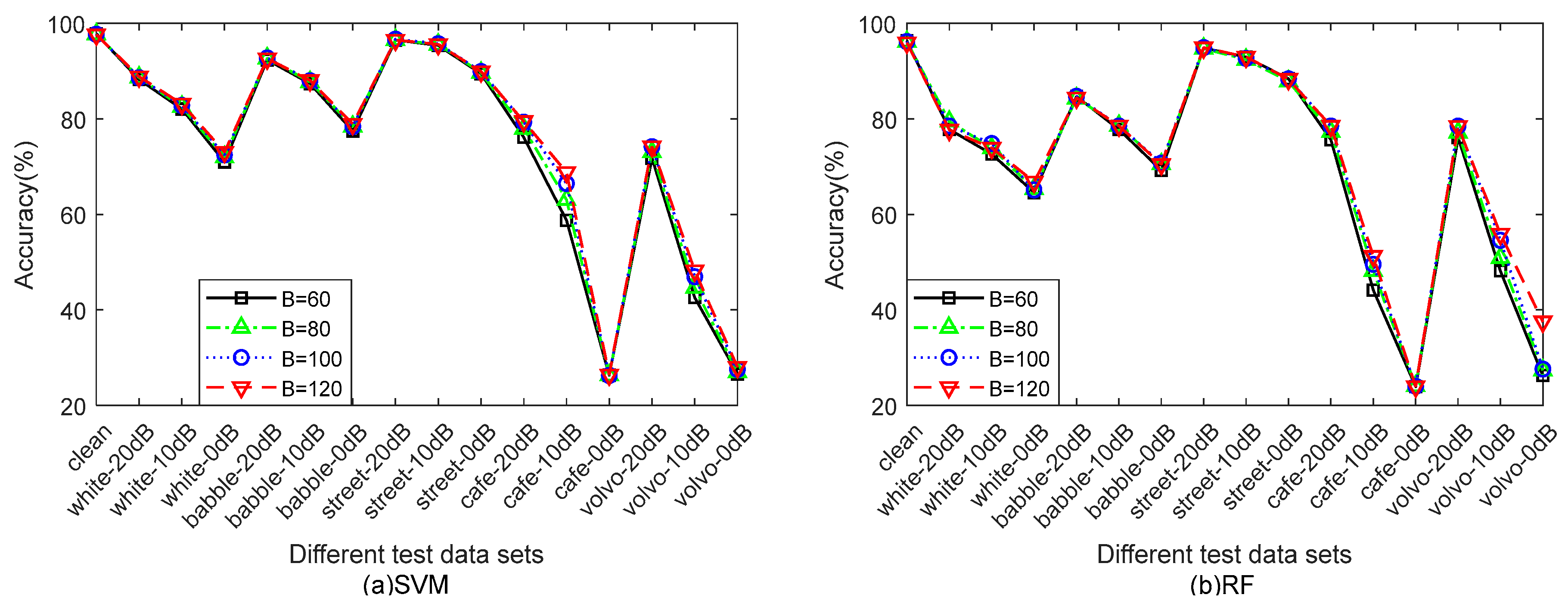
6.2. Parameter Setup
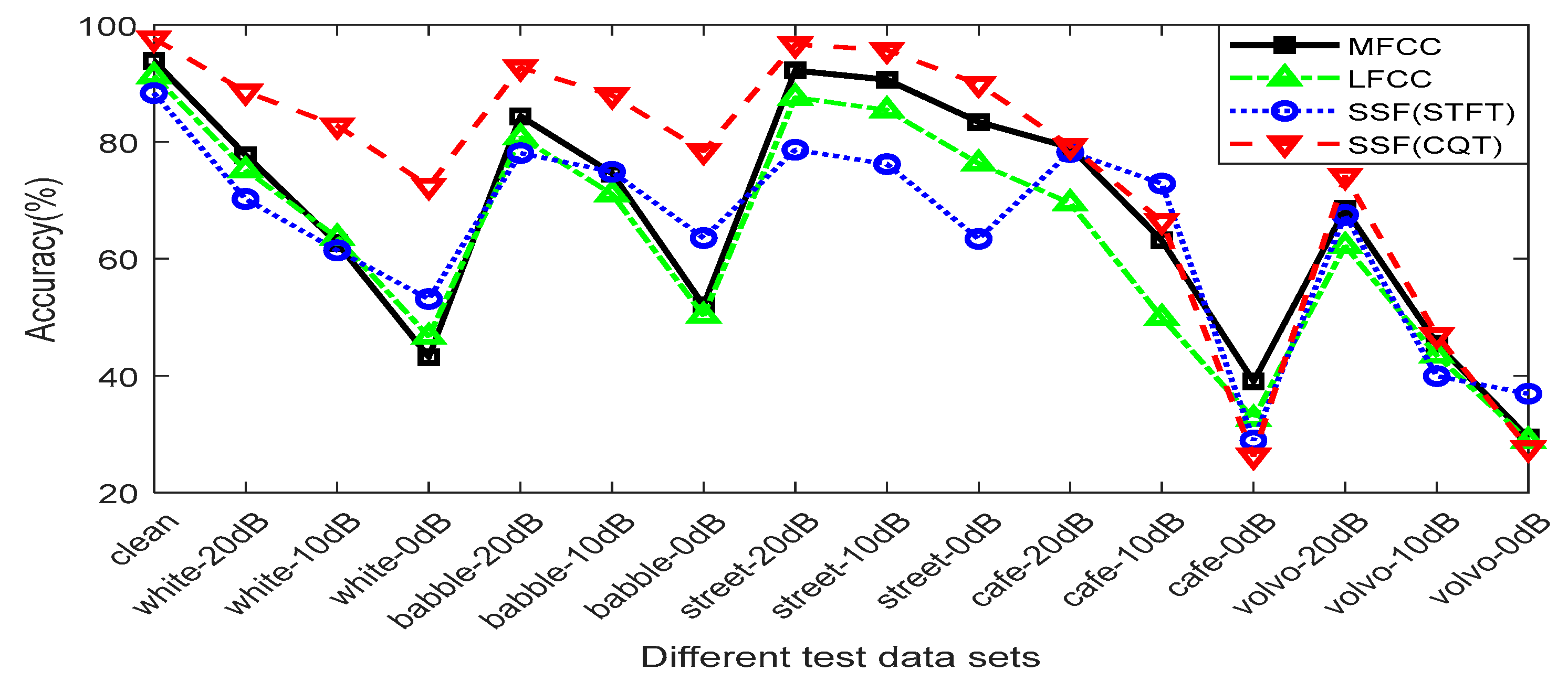
6.3. Comparison of Features
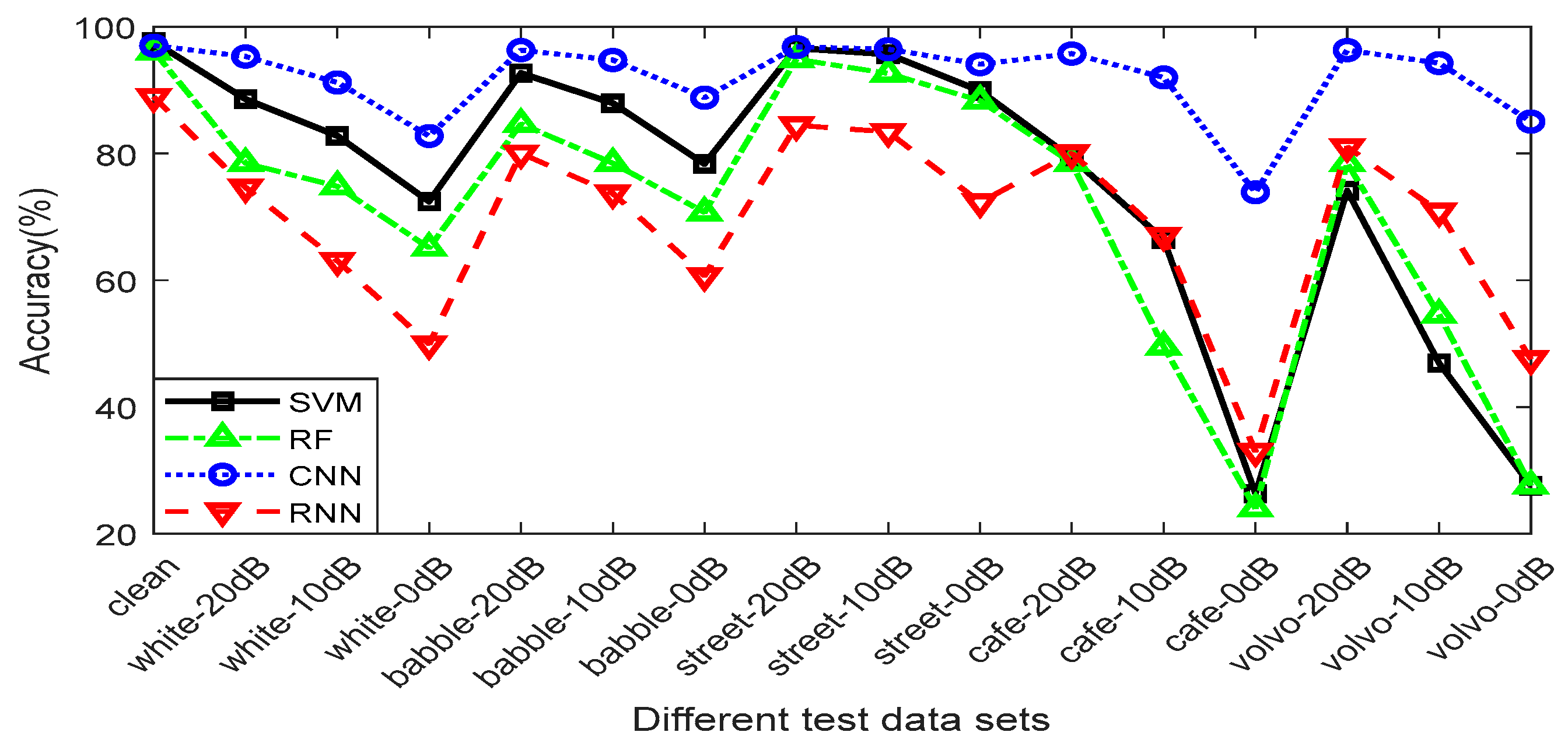
6.4. Comparison of Classifiers
6.5. Comparison of Single-Scene and Multi-Scene Training
6.6. Comparison of Different Identification Algorithms
7. Conclusions
Author Contributions
Funding
Conflicts of Interest
References
- Hanilci, C.; Ertas, F.; Ertas, T. Recognition of Brand and Models of Cell-Phones from Recorded Speech Signals. IEEE Trans. Inf. Forensics Secur. 2012, 7, 625–634. [Google Scholar] [CrossRef]
- Hanilçi, C.; Ertas, F. Optimizing Acoustic Features for Source Cell-Phone Recognition Using Speech Signals. In Proceedings of the First ACM Workshop on Information Hiding and Multimedia Security, Montpellier, France, 17–19 June 2013; pp. 141–148. [Google Scholar]
- Kotropoulos, C.; Samaras, S. Mobile Phone Identification Using Recorded Speech Signals. In Proceedings of the 19th International Conference on Digital Signal Processing, Hong Kong, China, 20–23 August 2014; pp. 586–591. [Google Scholar]
- Hanilçi, C.; Kinnunen, T. Source Cell-Phone Recognition from Recorded Speech Using Non-speech Segments. Digital Signal Process. 2014, 35, 75–85. [Google Scholar] [CrossRef]
- Zou, L.; Yang, J.; Huang, T. Automatic cell phone recognition from speech recordings. In Proceedings of the 2014 IEEE China Summit & International Conference on Signal and Information Processing (ChinaSIP), Xi’an, China, 9–13 July 2014; pp. 621–625. [Google Scholar]
- He, Q.; Wang, Z.; Rudnicky, A.I.; Li, X. A Recording Device Identification Algorithm Based on Improved PNCC Feature and Two-Step Discriminative Training. Electron. J. 2014, 42, 191–198. [Google Scholar]
- Kotropoulos, C. Telephone Handset Identification Using Sparse Representations of Spectral Feature Sketches. In Proceedings of the 2013 International Workshop on Biometrics and Forensics (IWBF), Lisbon, Portugal, 4–5 April 2013; pp. 1–4. [Google Scholar]
- Jin, C.; Wang, R.; Yan, D.; Tao, B.; Chen, Y.; Pei, A. Source Cell-Phone Identification Using Spectral Features of Device Self-noise. In Proceedings of the 15th International Workshop on Digital Watermarking (IWDW), Beijing, China, 17–19 September 2016; pp. 29–45. [Google Scholar]
- Qi, S.; Huang, Z.; Li, Y.; Shi, S. Audio Recording Device Identification Based on Deep Learning. In Proceedings of the 2016 IEEE International Conference on Signal and Image Processing (ICSIP), Beijing, China, 13–15 August 2016; pp. 426–431. [Google Scholar]
- Luo, D.; Korus, P.; Huang, J. Band Energy Difference for Source Attribution in Audio Forensics. IEEE Trans. Inf. Forensics Secur. 2018, 13, 2179–2189. [Google Scholar] [CrossRef]
- Jin, C. Research on Passive Forensics for Digital Audio. Ningbo University, 2016; pp. 28–35. Available online: http://cdmd.cnki.com.cn/Article/CDMD-11646-1017871275.htm (accessed on 17 August 2018).
- Garofolo, J.S.; Lamel, L.F.; Fisher, W.M.; Fiscus, J.G.; Pallett, D.S.; Dahlgren, N.L. DARPA TIMIT Acoustic-Phonetic Continuous Speech Corpus CD-ROM. NIST Speech Disc 1-1.1; U.S. Department of Commerce: Gaithersburg, MD, USA, 1993; p. 93.


| Class ID | Brand | Model | Class ID | Brand | Model |
|---|---|---|---|---|---|
| H1 | HTC | D610t | A1 | iPhone | iPhone 4s |
| H2 | D820t | A2 | iPhone 5 | ||
| H3 | One M7 | A3 | iPhone 5s | ||
| W1 | Huawei | Honor6 | A4 | iPhone 6 | |
| W2 | Honor7 | A5 | iPhone 6s | ||
| W3 | Mate7 | Z1 | Meizu | Meilan Note | |
| O1 | OPPO | Find7 | Z2 | MX2 | |
| O2 | Oneplus1 | Z3 | MX4 | ||
| O3 | R831S | M1 | Mi | Mi 3 | |
| S1 | Samsung | Galaxy Note2 | M2 | Mi 4 | |
| S2 | Galaxy S5 | M3 | Redmi Note1 | ||
| S3 | Galaxy GT-I8558 | M4 | Redmi Note2 |
| PL (Predict Label) | ||||||||||||||||||||||||
|---|---|---|---|---|---|---|---|---|---|---|---|---|---|---|---|---|---|---|---|---|---|---|---|---|
| AL | H1 | H2 | H3 | W1 | W2 | W3 | A1 | A2 | A3 | A4 | A5 | Z1 | Z2 | Z3 | M1 | M2 | M3 | M4 | O1 | O2 | O3 | S1 | S2 | S3 |
| H1 | 0.56 | 0.44 | 0 | 0 | 0 | 0 | 0 | 0 | 0 | 0 | 0 | 0 | 0 | 0 | 0 | 0 | 0 | 0 | 0 | 0 | 0 | 0 | 0 | 0 |
| H2 | 0.21 | 0.79 | 0 | 0 | 0 | 0 | 0 | 0 | 0 | 0 | 0 | 0 | 0 | 0 | 0 | 0 | 0 | 0 | 0 | 0 | 0 | 0 | 0 | 0 |
| H3 | 0.04 | 0.05 | 0.91 | 0 | 0 | 0 | 0 | 0 | 0 | 0 | 0 | 0 | 0 | 0 | 0 | 0 | 0 | 0 | 0 | 0 | 0 | 0 | 0 | 0 |
| W1 | 0 | 0 | 0 | 0.97 | 0 | 0.03 | 0 | 0 | 0 | 0 | 0 | 0 | 0 | 0 | 0 | 0 | 0 | 0 | 0 | 0 | 0 | 0 | 0 | 0 |
| W2 | 0 | 0 | 0 | 0.05 | 0.83 | 0.12 | 0 | 0 | 0 | 0 | 0 | 0 | 0 | 0 | 0 | 0 | 0 | 0 | 0 | 0 | 0 | 0 | 0 | 0 |
| W3 | 0 | 0 | 0 | 0.10 | 0 | 0.89 | 0 | 0 | 0 | 0 | 0 | 0 | 0 | 0 | 0 | 0 | 0 | 0 | 0 | 0 | 0 | 0.01 | 0 | 0 |
| A1 | 0 | 0 | 0 | 0 | 0 | 0 | 0.88 | 0 | 0.04 | 0.08 | 0 | 0 | 0 | 0 | 0 | 0 | 0 | 0 | 0 | 0 | 0 | 0 | 0 | 0 |
| A2 | 0 | 0 | 0 | 0 | 0 | 0 | 0 | 1.00 | 0 | 0 | 0 | 0 | 0 | 0 | 0 | 0 | 0 | 0 | 0 | 0 | 0 | 0 | 0 | 0 |
| A3 | 0 | 0 | 0 | 0 | 0 | 0 | 0.03 | 0 | 0.85 | 0.12 | 0 | 0 | 0 | 0 | 0 | 0 | 0 | 0 | 0 | 0 | 0 | 0 | 0 | 0 |
| A4 | 0 | 0 | 0 | 0 | 0 | 0 | 0.33 | 0 | 0.11 | 0.56 | 0 | 0 | 0 | 0 | 0 | 0 | 0 | 0 | 0 | 0 | 0 | 0 | 0 | 0 |
| A5 | 0 | 0 | 0 | 0 | 0 | 0 | 0 | 0 | 0 | 0 | 1.00 | 0 | 0 | 0 | 0 | 0 | 0 | 0 | 0 | 0 | 0 | 0 | 0 | 0 |
| Z1 | 0 | 0 | 0 | 0 | 0 | 0 | 0 | 0 | 0 | 0 | 0 | 1.00 | 0 | 0 | 0 | 0 | 0 | 0 | 0 | 0 | 0 | 0 | 0 | 0 |
| Z2 | 0 | 0 | 0 | 0 | 0 | 0 | 0 | 0 | 0 | 0 | 0 | 0 | 1.00 | 0 | 0 | 0 | 0 | 0 | 0 | 0 | 0 | 0 | 0 | 0 |
| Z3 | 0 | 0 | 0 | 0 | 0 | 0 | 0 | 0 | 0 | 0 | 0 | 0 | 0 | 1.00 | 0 | 0 | 0 | 0 | 0 | 0 | 0 | 0 | 0 | 0 |
| M1 | 0 | 0 | 0 | 0 | 0 | 0 | 0 | 0 | 0 | 0 | 0 | 0 | 0 | 0 | 1.00 | 0 | 0 | 0 | 0 | 0 | 0 | 0 | 0 | 0 |
| M2 | 0 | 0 | 0 | 0 | 0 | 0 | 0 | 0 | 0 | 0 | 0 | 0 | 0 | 0 | 0 | 1.00 | 0 | 0 | 0 | 0 | 0 | 0 | 0 | 0 |
| M3 | 0 | 0 | 0 | 0.01 | 0 | 0 | 0 | 0 | 0 | 0 | 0 | 0 | 0 | 0 | 0 | 0 | 0.99 | 0 | 0 | 0 | 0 | 0 | 0 | 0 |
| M4 | 0 | 0 | 0 | 0 | 0 | 0 | 0 | 0 | 0 | 0 | 0 | 0 | 0 | 0.01 | 0 | 0 | 0 | 0.83 | 0.15 | 0 | 0 | 0.01 | 0 | 0 |
| O1 | 0 | 0 | 0 | 0 | 0 | 0 | 0 | 0 | 0 | 0 | 0 | 0 | 0 | 0 | 0.01 | 0 | 0 | 0 | 0.99 | 0 | 0 | 0 | 0 | 0 |
| O2 | 0 | 0 | 0 | 0 | 0 | 0 | 0 | 0 | 0 | 0 | 0 | 0 | 0 | 0 | 0 | 0 | 0 | 0 | 0 | 1.00 | 0 | 0 | 0 | 0 |
| O3 | 0 | 0 | 0 | 0 | 0 | 0 | 0 | 0 | 0 | 0 | 0 | 0 | 0 | 0 | 0 | 0 | 0 | 0 | 0 | 0 | 1.00 | 0 | 0 | 0 |
| S1 | 0 | 0 | 0 | 0 | 0 | 0 | 0 | 0 | 0 | 0 | 0 | 0 | 0 | 0 | 0.04 | 0 | 0 | 0 | 0.01 | 0 | 0 | 0.95 | 0 | 0 |
| S2 | 0 | 0 | 0 | 0.01 | 0.01 | 0 | 0 | 0 | 0 | 0 | 0 | 0 | 0 | 0 | 0 | 0 | 0 | 0 | 0 | 0 | 0 | 0 | 0.98 | 0 |
| S3 | 0 | 0 | 0 | 0 | 0 | 0 | 0 | 0 | 0 | 0 | 0 | 0.08 | 0 | 0.02 | 0 | 0 | 0 | 0 | 0 | 0 | 0 | 0 | 0 | 0.90 |
| PL (Predict Label) | ||||||||||||||||||||||||
|---|---|---|---|---|---|---|---|---|---|---|---|---|---|---|---|---|---|---|---|---|---|---|---|---|
| AL | H1 | H2 | H3 | W1 | W2 | W3 | A1 | A2 | A3 | A4 | A5 | Z1 | Z2 | Z3 | M1 | M2 | M3 | M4 | O1 | O2 | O3 | S1 | S2 | S3 |
| H1 | 0.87 | 0.13 | 0 | 0 | 0 | 0 | 0 | 0 | 0 | 0 | 0 | 0 | 0 | 0 | 0 | 0 | 0 | 0 | 0 | 0 | 0 | 0 | 0 | 0 |
| H2 | 0.14 | 0.86 | 0 | 0 | 0 | 0 | 0 | 0 | 0 | 0 | 0 | 0 | 0 | 0 | 0 | 0 | 0 | 0 | 0 | 0 | 0 | 0 | 0 | 0 |
| H3 | 0 | 0 | 1.00 | 0 | 0 | 0 | 0 | 0 | 0 | 0 | 0 | 0 | 0 | 0 | 0 | 0 | 0 | 0 | 0 | 0 | 0 | 0 | 0 | 0 |
| W1 | 0 | 0 | 0 | 0.97 | 0.02 | 0.01 | 0 | 0 | 0 | 0 | 0 | 0 | 0 | 0 | 0 | 0 | 0 | 0 | 0 | 0 | 0 | 0 | 0 | 0 |
| W2 | 0 | 0 | 0 | 0.01 | 0.96 | 0.03 | 0 | 0 | 0 | 0 | 0 | 0 | 0 | 0 | 0 | 0 | 0 | 0 | 0 | 0 | 0 | 0 | 0 | 0 |
| W3 | 0 | 0 | 0 | 0 | 0 | 1.00 | 0 | 0 | 0 | 0 | 0 | 0 | 0 | 0 | 0 | 0 | 0 | 0 | 0 | 0 | 0 | 0 | 0 | 0 |
| A1 | 0 | 0 | 0 | 0 | 0 | 0 | 0.98 | 0 | 0.02 | 0 | 0 | 0 | 0 | 0 | 0 | 0 | 0 | 0 | 0 | 0 | 0 | 0 | 0 | 0 |
| A2 | 0 | 0 | 0 | 0 | 0 | 0 | 0 | 1.00 | 0 | 0 | 0 | 0 | 0 | 0 | 0 | 0 | 0 | 0 | 0 | 0 | 0 | 0 | 0 | 0 |
| A3 | 0 | 0 | 0 | 0 | 0 | 0 | 0.05 | 0 | 0.92 | 0.02 | 0.01 | 0 | 0 | 0 | 0 | 0 | 0 | 0 | 0 | 0 | 0 | 0 | 0 | 0 |
| A4 | 0 | 0 | 0 | 0 | 0 | 0 | 0.04 | 0.04 | 0 | 0.92 | 0 | 0 | 0 | 0 | 0 | 0 | 0 | 0 | 0 | 0 | 0 | 0 | 0 | 0 |
| A5 | 0 | 0 | 0 | 0 | 0 | 0 | 0 | 0 | 0 | 0 | 1.00 | 0 | 0 | 0 | 0 | 0 | 0 | 0 | 0 | 0 | 0 | 0 | 0 | 0 |
| Z1 | 0 | 0 | 0 | 0 | 0 | 0 | 0 | 0 | 0 | 0 | 0 | 1.00 | 0 | 0 | 0 | 0 | 0 | 0 | 0 | 0 | 0 | 0 | 0 | 0 |
| Z2 | 0 | 0 | 0 | 0 | 0.01 | 0 | 0 | 0 | 0 | 0 | 0 | 0 | 0.99 | 0 | 0 | 0 | 0 | 0 | 0 | 0 | 0 | 0 | 0 | 0 |
| Z3 | 0 | 0 | 0 | 0 | 0 | 0 | 0 | 0 | 0 | 0 | 0 | 0 | 0 | 1.00 | 0 | 0 | 0 | 0 | 0 | 0 | 0 | 0 | 0 | 0 |
| M1 | 0 | 0 | 0 | 0 | 0 | 0 | 0 | 0 | 0 | 0 | 0 | 0 | 0 | 0 | 1.00 | 0 | 0 | 0 | 0 | 0 | 0 | 0 | 0 | 0 |
| M2 | 0 | 0 | 0 | 0 | 0 | 0 | 0 | 0 | 0 | 0 | 0 | 0 | 0 | 0 | 0 | 1.00 | 0 | 0 | 0 | 0 | 0 | 0 | 0 | 0 |
| M3 | 0 | 0 | 0 | 0 | 0 | 0 | 0 | 0 | 0 | 0 | 0 | 0 | 0 | 0 | 0 | 0 | 1.00 | 0 | 0 | 0 | 0 | 0 | 0 | 0 |
| M4 | 0 | 0 | 0 | 0 | 0 | 0 | 0 | 0 | 0 | 0 | 0 | 0 | 0 | 0 | 0 | 0 | 0 | 1.00 | 0 | 0 | 0 | 0 | 0 | 0 |
| O1 | 0 | 0 | 0 | 0 | 0 | 0 | 0 | 0 | 0 | 0 | 0 | 0 | 0 | 0 | 0 | 0 | 0 | 0 | 1.00 | 0 | 0 | 0 | 0 | 0 |
| O2 | 0 | 0 | 0 | 0 | 0 | 0 | 0 | 0 | 0 | 0 | 0 | 0 | 0 | 0 | 0 | 0 | 0 | 0 | 0 | 1.00 | 0 | 0 | 0 | 0 |
| O3 | 0 | 0 | 0 | 0 | 0 | 0 | 0 | 0 | 0 | 0 | 0 | 0 | 0 | 0 | 0 | 0 | 0 | 0 | 0 | 0 | 1.00 | 0 | 0 | 0 |
| S1 | 0 | 0 | 0 | 0 | 0 | 0 | 0 | 0 | 0 | 0 | 0 | 0 | 0 | 0 | 0 | 0 | 0 | 0 | 0 | 0 | 0 | 1.00 | 0 | 0 |
| S2 | 0 | 0 | 0 | 0 | 0 | 0 | 0 | 0 | 0 | 0 | 0 | 0 | 0 | 0 | 0 | 0 | 0 | 0 | 0 | 0 | 0 | 0 | 1.00 | 0 |
| S3 | 0 | 0 | 0 | 0 | 0 | 0 | 0 | 0 | 0 | 0 | 0 | 0 | 0 | 0 | 0 | 0 | 0 | 0 | 0 | 0 | 0 | 0 | 0 | 1.00 |
| Brands | Clean | White_0dB | ||
|---|---|---|---|---|
| MFCC | SSF (CQT) | MFCC | SSF (CQT) | |
| HTC | 75.33% | 91.00% | 49.17% | 70.33% |
| Huawei | 89.67% | 97.67% | 68.83% | 77.17% |
| iPhone | 85.80% | 96.40% | 36.10% | 56.70% |
| Meizu | 100% | 99.67% | 33.31% | 69.50% |
| Mi | 95.50% | 100% | 31.13% | 85.25% |
| OPPO | 99.67% | 100% | 31.00% | 82.83% |
| Samsung | 94.34% | 100% | 43.33% | 71.67% |
| Test Data Sets | Single | Multiple | ||
|---|---|---|---|---|
| CKC-SD | TIMIT-RD | CKC-SD | TIMIT-RD | |
| Seen Noisy Scenarios | ||||
| clean | 95.47% | 98.89% | 97.08% | 99.29% |
| white_20dB | 54.80% | 58.80% | 95.35% | 96.31% |
| white_10dB | 36.11% | 35.11% | 91.25% | 91.99% |
| white _0dB | 18.50% | 16.50% | 82.79% | 84.57% |
| babble_20dB | 76.71% | 77.71% | 96.35% | 97.54% |
| babble 10dB | 49.92% | 50.92% | 94.79% | 96.03% |
| babble_0dB | 26.77% | 29.77% | 88.85% | 90.23% |
| street_20dB | 97.86% | 98.86% | 96.85% | 98.44% |
| street_10dB | 86.27% | 87.27% | 96.50% | 97.40% |
| street_0dB | 54.81% | 52.81% | 94.13% | 93.47% |
| Unseen Noisy Scenarios | ||||
| cafe_20dB | 88.33% | 89.99% | 95.81% | 96.56% |
| cafe_10dB | 56.25% | 61.25% | 92.04% | 94.63% |
| cafe_0dB | 30.75% | 27.75% | 73.90% | 76.43% |
| volvo_20dB | 92.33% | 93.33% | 96.35% | 96.34% |
| volvo_10dB | 71.98% | 76.98% | 94.30% | 92.21% |
| volvo_0dB | 45.75% | 46.75% | 85.06% | 88.06% |
| Test Data Sets | This Paper | Reference [10] | ||
|---|---|---|---|---|
| CKC-SD | TIMIT-RD | CKC-SD | TIMIT-RD | |
| Seen Noisy Scenarios | ||||
| clean | 97.08% | 99.29% | 97.04% | 98.69% |
| white_20dB | 95.35% | 96.31% | 89.60% | 88.60% |
| white_10dB | 91.25% | 91.99% | 84.29% | 82.82% |
| white _0dB | 82.79% | 84.57% | 76.62% | 72.46% |
| babble_20dB | 96.35% | 97.54% | 92.29% | 92.73% |
| babble 10dB | 94.79% | 96.03% | 88.46% | 87.98% |
| babble_0dB | 88.85% | 90.23% | 79.73% | 78.40% |
| street_20dB | 96.85% | 98.44% | 96.19% | 96.69% |
| street_10dB | 96.50% | 97.40% | 95.38% | 95.73% |
| street_0dB | 94.13% | 93.47% | 89.81% | 89.90% |
| Unseen Noisy Scenarios | ||||
| cafe_20dB | 95.81% | 96.56% | 79.74% | 79.31% |
| cafe_10dB | 92.04% | 94.63% | 63.73% | 66.46% |
| cafe_0dB | 73.90% | 76.43% | 25.19% | 26.27% |
| volvo_20dB | 96.35% | 96.34% | 64.32% | 74.17% |
| volvo_10dB | 94.30% | 92.21% | 32,92% | 46.94% |
| volvo_0dB | 85.06% | 88.06% | 17.85% | 27.54% |
© 2018 by the authors. Licensee MDPI, Basel, Switzerland. This article is an open access article distributed under the terms and conditions of the Creative Commons Attribution (CC BY) license (http://creativecommons.org/licenses/by/4.0/).
Share and Cite
Qin, T.; Wang, R.; Yan, D.; Lin, L. Source Cell-Phone Identification in the Presence of Additive Noise from CQT Domain. Information 2018, 9, 205. https://doi.org/10.3390/info9080205
Qin T, Wang R, Yan D, Lin L. Source Cell-Phone Identification in the Presence of Additive Noise from CQT Domain. Information. 2018; 9(8):205. https://doi.org/10.3390/info9080205
Chicago/Turabian StyleQin, Tianyun, Rangding Wang, Diqun Yan, and Lang Lin. 2018. "Source Cell-Phone Identification in the Presence of Additive Noise from CQT Domain" Information 9, no. 8: 205. https://doi.org/10.3390/info9080205
APA StyleQin, T., Wang, R., Yan, D., & Lin, L. (2018). Source Cell-Phone Identification in the Presence of Additive Noise from CQT Domain. Information, 9(8), 205. https://doi.org/10.3390/info9080205